Technical Note: On the puzzling similarity of two water balance formulas – Turc–Mezentsev vs. Tixeront–Fu

This Technical Note documents and analyzes the puzzling similarity of two widely used water balance formulas: Turc–Mezentsev and Tixeront–Fu. It details their history and their hydrological and mathematical properties, and discusses the mathematical reasoning behind their slight differences. Apart from the difference in their partial differential expressions, both formulas share the same hydrological properties, and it seems impossible to recommend one over the other as more “hydrologically founded”: hydrologists should feel free to choose the one they feel more comfortable with.

1 Introduction

The Turc–Mezentsev (Mezentsev, 1955; Turc, 1954) and Tixeront–Fu (Fu, 1981; Tixeront, 1964) formulas were introduced to model long-term water balance at the catchment scale. Both formulas are almost equivalent numerically (but differ nonetheless). Surprisingly, comparisons are rare: Tixeront knew the work of Turc (1954), which he cites, but it seems that he did not realize that Turc's formulation was numerically equivalent to the one he proposed. Similarly, Fu knew the work of Mezentsev (1955) because he precisely starts his 1981 paper by discussing it, but it seems that he did not realize that the formulation he obtained was so close numerically.

As far as we know, Yang et al. (2008) were the first to compare the Turc–Mezentsev and Tixeront–Fu formulas and to conclude that both formulas were “approximately equivalent”. In this note we further elaborate on the similarity between the two formulas and contribute complementary explanations of their underlying hypotheses.

2 Presentation of the Turc–Mezentsev (TM) and Tixeront–Fu (TF) formulas

The TM and TF formulas use as inputs long-term average precipitation P (mm yr⁻¹) and long-term average maximum evaporation E₀ (mm yr⁻¹). They produce as outputs either long-term average specific streamflow Q (mm yr⁻¹) or long-term average actual evaporation E (mm yr⁻¹). There are two formulations (one giving Q as a function of P and E₀ and one giving E as a function of the same variables), equivalent under the assumption that the catchment is conservative (i.e., that it does not “leak” towards deep aquifers) so that E and Q can be linked through the equation $E=P-Q$. Maximum evaporation is understood in the sense of Budyko (1963/1948) as the water equivalent of the energy available to evaporation. In what follows, the E₀∕P ratio is called the aridity ratio; its inverse (i.e., the P∕E₀ ratio) is called the humidity ratio. The formulas are presented in Table 1. Because none of the original papers introducing them are in English, we also document their origins in the Appendix, in order to provide interested readers with a more detailed description of the origin of each formula.

Table 1 Turc–Mezentsev (TM) and Tixeront–Fu (TF) water–energy balance formulations (P – precipitation, Q – streamflow, E₀ – maximum evaporation, E – actual evaporation, all in mm yr⁻¹ averaged over many years). n is the free parameter of the Turc–Mezentsev formula (n>0); m is the free parameter of the Tixeront–Fu formula (m>1).

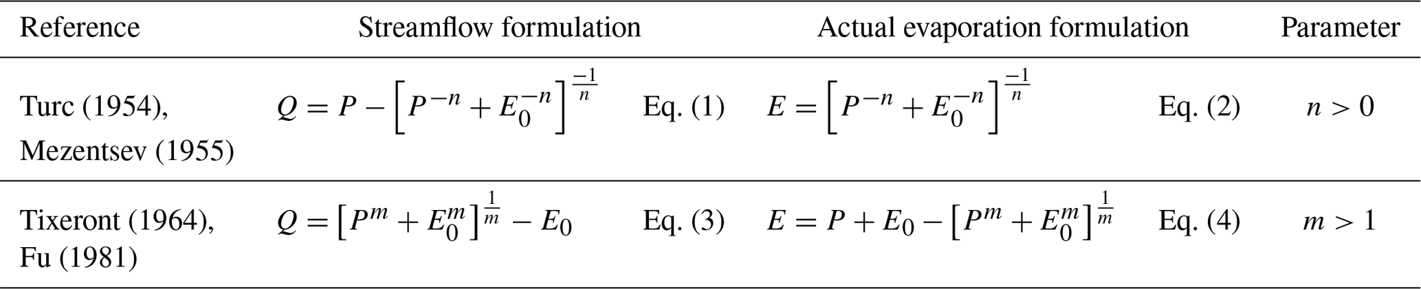
Table 2 Partial derivatives of the Turc–Mezentsev formula (P – precipitation, Q – streamflow, E₀ – maximum evaporation, E – actual evaporation, all in mm yr⁻¹ averaged over many years). n is the free parameter of the Turc–Mezentsev formula (n>0).

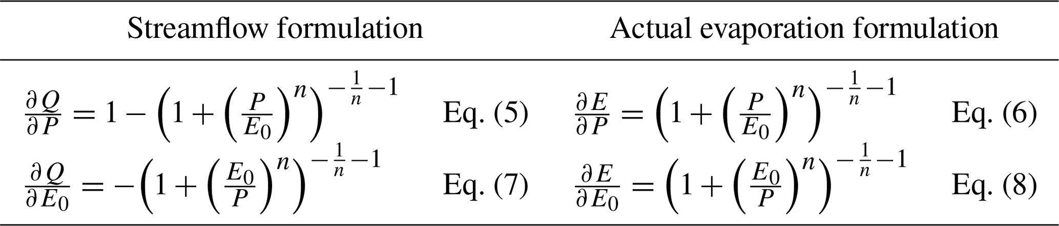
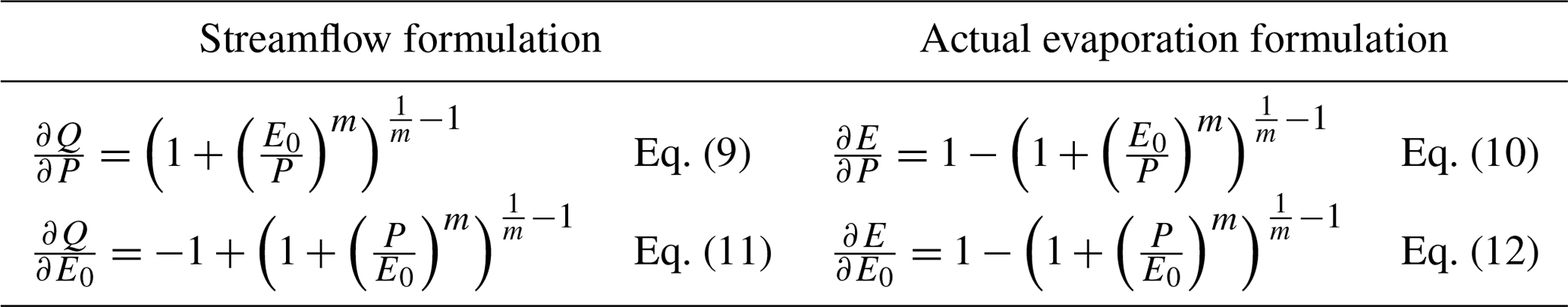
Table 3 Partial derivatives of the Tixeront–Fu formula (P – precipitation, Q – streamflow, E₀ – maximum evaporation, E – actual evaporation, all in mm yr⁻¹ averaged over many years). m is the free parameter of the Tixeront–Fu formula (m>1).

We need to clarify here that the TM and TF formulas can be found in the hydrologic literature under different names. The naming convention we adopted is explained as follows: Eqs. (1) and (2) are named “Turc–Mezentsev” (TM) because Turc (1954) and Mezentsev (1955) worked independently and published the same equation almost simultaneously. Equations (3) and (4) are named “Tixeront–Fu” (TF) because although Tixeront's original publication predates Fu's by almost 20 years, both publications were independent, and the name of Fu has already gained wide international recognition. Both formulas are sometimes referred to as “Budyko-type,” although none of them were actually used by Budyko (1963/1948), who instead used a parameter-free formula derived from the work of Oldekop (1911) (for a synthesis of Oldekop's work and how it was used by Budyko, see Andréassian et al., 2016). Other authors have published papers containing the TM formula (see, e.g., Hsuen-Chun, 1988, and Choudhury, 1999), and their names are sometimes used to designate it.

In our interpretation of the TM and TF formulas, we will use their partial derivatives, which we present in Tables 2 and 3.

3 Comparisons of the Turc–Mezentsev and Tixeront–Fu formulas

3.1 Previous comparisons

We mentioned in the introduction that the first paper comparing the TM and TF formulas was published by Yang et al. (2008), who note that the TM and TF formulas are “approximately equivalent” and that their parameters have a “perfectly significant linear correlation relationship”, which they identify as in Eq. (13):

$$\begin{array}{}\text{(13)}& {\displaystyle }{\displaystyle }m\sim n+\mathrm{0.72},\end{array}$$

where m stands for the parameter of the Tixeront–Fu relationship and n for the parameter of the Turc–Mezentsev relationship.

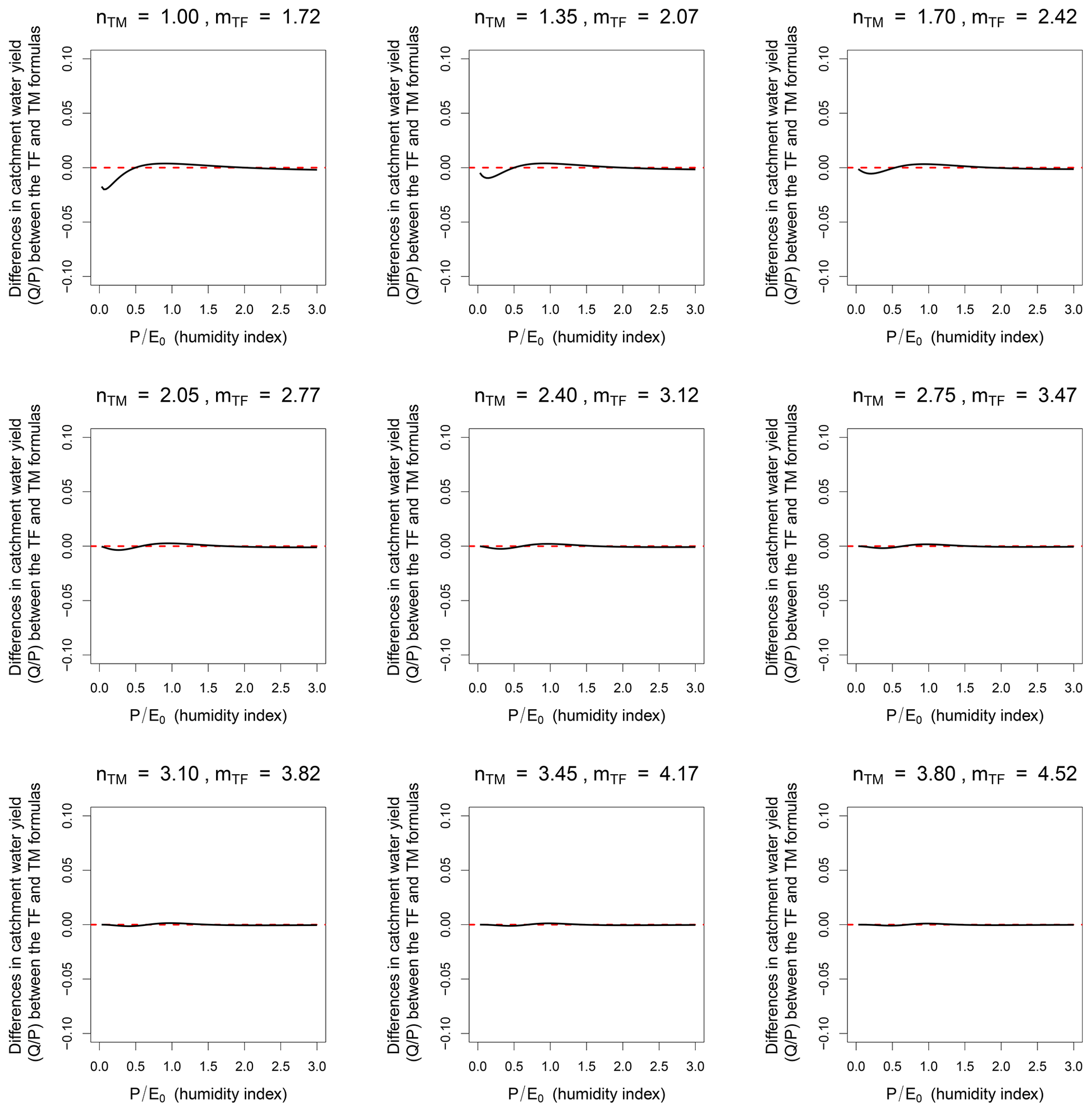
Figure 1 Illustration of the similarity between the values of the Turc–Mezentsev (TM) and Tixeront–Fu (TF) formulas for a range of values of n (the parameter of the TM formula) and m (the parameter of the TF formula), using the Yang et al. (2008) relationship: $m=n+\mathrm{0.72}$.

Note that Eq. (13) is an experimental relationship obtained by regression. It gives slightly more satisfying results than the “theoretical” relationship (found by equating both equations for $P/E_{\mathrm{0}}=\mathrm{1}$) given below (Eq. 14):

$$\begin{array}{}\text{(14)}& {\displaystyle }{\displaystyle }m={\displaystyle \frac{\ln \mathrm{2}}{\ln \left[\mathrm{2}-{\mathrm{2}}^{\frac{-\mathrm{1}}{n}}\right]}}.\end{array}$$

Recently, Andréassian et al. (2016) and de Lavenne and Andréassian (2018) used the Yang et al. (2008) results and further illustrated the nearly perfect similarity between the two formulas.

3.2 Graphical illustration of the similarity of the TM and TF formulas

Figure 1, which illustrates the numerical proximity of the two formulas, speaks for itself: while we tested a wide range of (n, m) couples respecting Eq. (13), the difference (TM − TF) between the two formulas is at maximum 2.5 %, and most of the time much less. Numerically, both formulas are equivalent (except for very low values of the humidity index P∕E₀).

Figure 2 Illustration of the similarity between the Turc–Mezentsev (TM) and Tixeront–Fu (TF) formulas for a range of values of n (the parameter of the TM formula) and m (the parameter of the TF formula), using the Yang et al. (2008) relationship: $m=n+\mathrm{0.72}$: difference in the partial differentials $\frac{\partial E}{\partial P}$.

Figures 2 and 3 also present the differences between the partial derivatives of the TM and TF formulas. The reason for this is that both formulas are sometimes used to predict the hydrological impact of climatic change, i.e., to evaluate the evolution or differences between future and current conditions. Again, both formulas appear numerically equivalent.

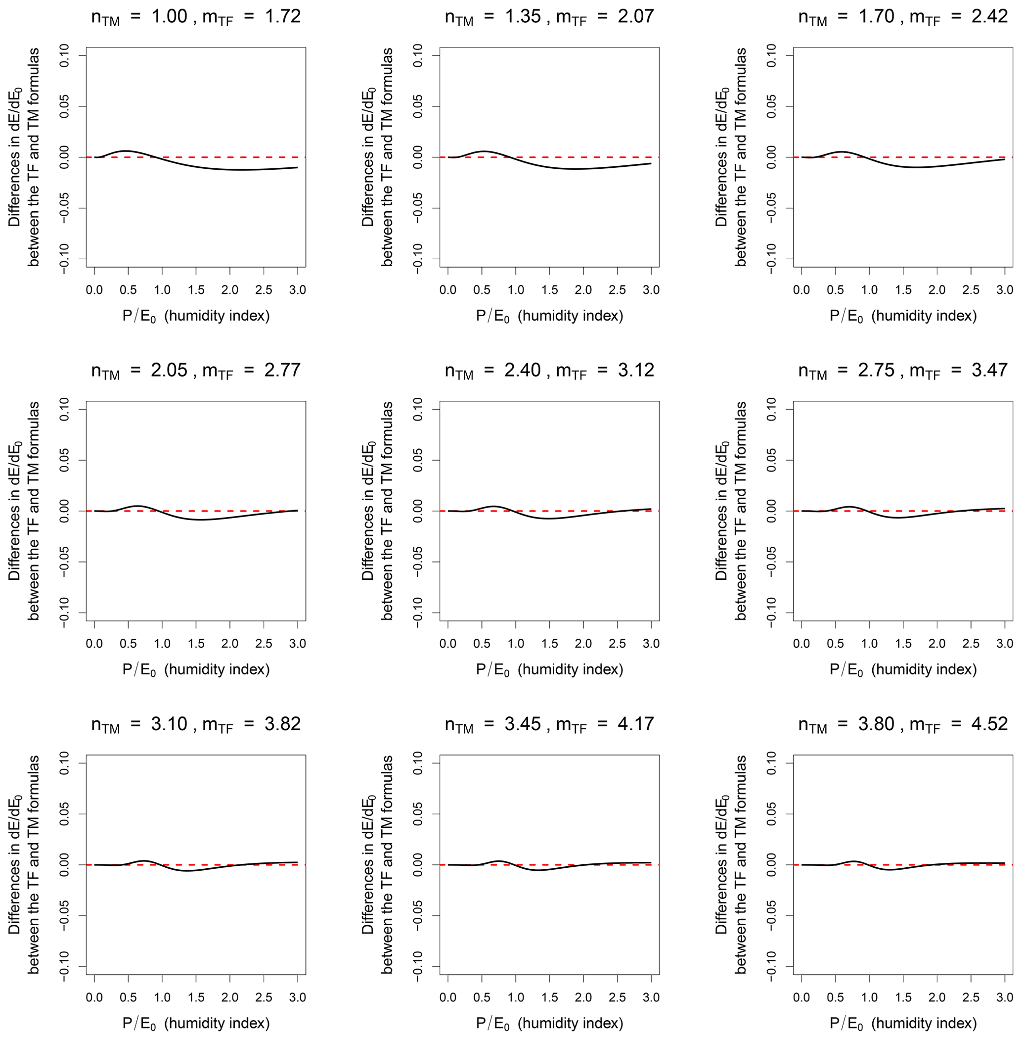
Figure 3 Illustration of the similarity between the Turc–Mezentsev (TM) and Tixeront–Fu (TF) formulas for a range of values of n (the parameter of the TM formula) and m (the parameter of the TF formula), using the Yang et al. (2008) relationship: $m=n+\mathrm{0.72}$: difference in the partial differentials $\frac{\partial E}{\partial E_{\mathrm{0}}}$.

4 Interpretation of the TM and TF formulas

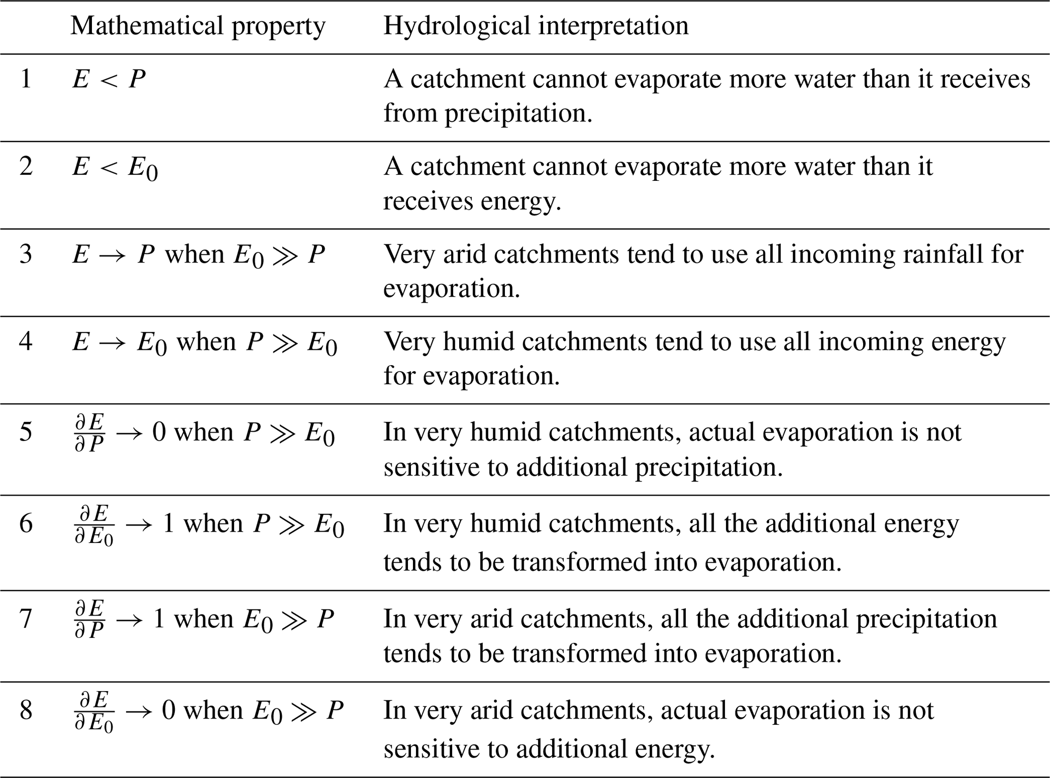
4.1 Hydrological interpretation

The TM and TF formulas share a set of hydrological properties that we summarize in Tables 4 and 5, following the presentation proposed by Lebecherel et al. (2013).

Table 4 Hydrological interpretation of the Turc–Mezentsev and Tixeront–Fu formulas, applied to streamflow (P – precipitation, Q – streamflow, E₀ – maximum evaporation, all in mm yr⁻¹ averaged over many years).

Table 5 Hydrological interpretation of the Turc–Mezentsev and Tixeront–Fu formulas, applied to actual evaporation (P – precipitation, E₀ – maximum evaporation, E – actual evaporation, all in mm yr⁻¹ averaged over many years).

4.2 Mathematical interpretation

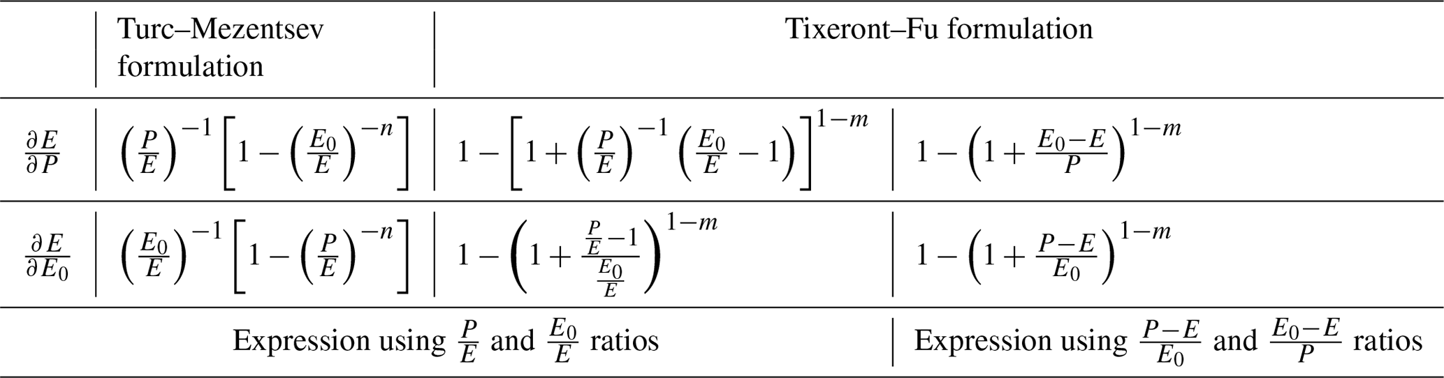
The Appendix summarizes the underlying mathematical reasoning presented by the authors of the TM and TF formulas and by Zhang et al. (2004) and Yang et al. (2008). What can be concluded from the analysis presented in the Appendix is that both formulations are based on very similar but nonetheless slightly different hypotheses: Table 6 illustrates them after rewriting the partial differentials to make E appear (for the TM formula, see Yang et al., 2008, and Eqs. A16 and A17 in Appendix; for the TF formula see Fu, 1981, and Eqs. A9 and A10 in the Appendix):

• For the Turc–Mezentsev formula, Table 6 shows that $\frac{\partial E}{\partial P}$ and $\frac{\partial E}{\partial E_{\mathrm{0}}}$ can only be written as functions of the $\frac{P}{E}$ and $\frac{E_{\mathrm{0}}}{E}$ ratios.

• For the Tixeront–Fu formula, Table 6 shows that $\frac{\partial E}{\partial P}$ and $\frac{\partial E}{\partial E_{\mathrm{0}}}$ can be written as functions of the $\frac{P}{E}$ and $\frac{E_{\mathrm{0}}}{E}$ ratios (as for the TM formulation). But in addition, $\frac{\partial E}{\partial P}$ can be written as a function of $\frac{E_{\mathrm{0}}-E}{P}$ (i.e., the remaining energy divided by P) and $\frac{\partial E}{\partial E_{\mathrm{0}}}$ can be written as a function of $\frac{P-E}{E_{\mathrm{0}}}$ (the remaining water divided by E₀). In fact, Fu (1981) demonstrated in a rigorous mathematical way that the TF formulation was the only possible solution to this set of hypotheses (i.e., Eq. A6 in the Appendix).

Table 6 Comparison of the partial differentials of the Turc–Mezentsev and Tixeront–Fu formulas (P – precipitation, E₀ – maximum evaporation, E – actual evaporation, all in mm yr⁻¹ averaged over many years; n is the free parameter of the Turc–Mezentsev formula (n>0); m is the free parameter of the Tixeront–Fu formula (m>1)).

What can we conclude from this? Does this make the TF formula (slightly) more general and the TM formula (slightly) more restrictive? Perhaps, but from the user's point of view, both formulas are so close numerically (see Fig. 1 and also compare the maps presented by de Lavenne and Andréassian, 2018) that any data-based distinction is impossible.

5 Conclusion

The Turc–Mezentsev and Tixeront–Fu formulas are two sound and numerically equivalent representations of the long-term water balance at the catchment scale. This note investigated the underlying assumptions of the two formulas and showed that the Tixeront–Fu formula is slightly more general than the Turc–Mezentsev formula, because its partial differences can be written both as a function of the $\frac{P}{E}$ and $\frac{E_{\mathrm{0}}}{E}$ ratios and as a function of the $\frac{E_{\mathrm{0}}-E}{P}$ and $\frac{P-E}{E_{\mathrm{0}}}$ ratios (the TM formula can only write its partial differences as a function of the $\frac{P}{E}$ and $\frac{E_{\mathrm{0}}}{E}$ ratios). Apart from this difference, both formulas share the same hydrological properties and we can see no reason to recommend one over the other as more “hydrologically founded”. This should not be considered disappointing: it simply means that hydrologists should feel free to choose the formula they feel more comfortable with.

Appendix A: Supplementary genealogical and mathematical considerations concerning the Turc–Mezentsev and Tixeront–Fu formulations

A1 Origin of the Turc formula

Lucien Turc was a French soil scientist. He produced his formula while working on his PhD thesis, defended in April 1953 (and published in 1954 in the Annales Agronomiques). Turc used water balance data for a set of 254 catchments from all over the world, collected with the help of Maurice Pardé, a well-known hydrologist of that time. He computed catchment-scale long-term average actual evaporation (E) from estimates of long-term average precipitation (P) and long-term average streamflow (Q) by writing $E=P-Q$ (all variables in mm yr⁻¹), and he used a polynomial relationship to compute E₀ from temperature. After plotting his catchment data in the $E/E_{\mathrm{0}}=f(P/E_{\mathrm{0}})$ nondimensional space, Turc looked for a mathematical function running through the experimental points and respecting the two following constraints:

• $\frac{E}{E_{\mathrm{0}}}\sim \frac{P}{E_{\mathrm{0}}}$ when $\frac{P}{E_{\mathrm{0}}}$ is small,

• $\frac{E}{E_{\mathrm{0}}}\sim \mathrm{1}$ when $\frac{P}{E_{\mathrm{0}}}$ is large.

Turc (1954, p. 504) wrote that the simplest function respecting these two conditions would be

$${\displaystyle }{\displaystyle }y={\displaystyle \frac{x}{\mathrm{1}+x}},\mathrm{with}y={\displaystyle \frac{E}{E_{\mathrm{0}}}}\mathrm{and}x={\displaystyle \frac{P}{E_{\mathrm{0}}}},$$

and that the most general would be

$$\begin{array}{ll}{\displaystyle }& {\displaystyle }y={\displaystyle \frac{x}{{\left(\mathrm{1}+x^n\right)}^{\frac{\mathrm{1}}{n}}}},\mathrm{i}.\mathrm{e}.,{\displaystyle \frac{E}{E_{\mathrm{0}}}}={\displaystyle \frac{\frac{P}{E_{\mathrm{0}}}}{{\left[\mathrm{1}+{\left(\frac{P}{E_{\mathrm{0}}}\right)}^n\right]}^{\frac{\mathrm{1}}{n}}}}\\ \text{(A1)}& {\displaystyle }& {\displaystyle }\mathrm{or}{\displaystyle \frac{E}{P}}={\displaystyle \frac{\mathrm{1}}{{\left[\mathrm{1}+{\left(\frac{P}{E_{\mathrm{0}}}\right)}^n\right]}^{\frac{\mathrm{1}}{n}}}},\end{array}$$

in which n is an exponent to estimate. Turc graphically looked for the most convenient value for n and concluded that the best fit was “with n=3, or maybe n=2” (Turc, 1954, p. 563). Since the choice of n=2 allowed the simplest computations, he retained this value for further developments.

A2 Origin of the Mezentsev formula

Varfolomeï Mezentsev was a Soviet geographer, working at the University of Omsk in Siberia. He published his formula in 1955, and continued working on it throughout his life (Mezentsev, 1955, 1982, 1993). Mezentsev (1955, 1982, 1993) started his analysis from a formula proposed by Bagrov (1953) (Eq. A2):

$$\begin{array}{}\text{(A2)}& {\displaystyle }{\displaystyle \frac{\mathrm{d}E}{\mathrm{d}P}}=\mathrm{1}-{\left({\displaystyle \frac{E}{E_{\mathrm{0}}}}\right)}^n.\end{array}$$

The Bagrov formula can be interpreted as follows: when $\frac{E}{E_{\mathrm{0}}}$ is small, i.e., when water is the limiting factor, an increase in precipitation P is integrally transformed into an increase in actual evaporation E. Conversely, when $\frac{E}{E_{\mathrm{0}}}$ approaches 1 (i.e., when water does not limit evaporation), none of the additional P is transformed into E because no more energy is available for evaporation. Bagrov showed that this formula presents the interesting property of integrating into the Oldekop (1911) water balance formula for n=2. For n=1, $n=\mathrm{4}/\mathrm{3}$ and $n=\mathrm{3}/\mathrm{2}$, Bagrov found analytical solutions, but he could not find a generic solution for all values of n.

Mezentsev (1955) reasoned that in order to find a generic solution, Bagrov's formula could be rewritten as follows:

$$\begin{array}{}\text{(A3)}& {\displaystyle }{\displaystyle \frac{\mathrm{d}E}{\mathrm{d}P}}={\left[\mathrm{1}-{\left({\displaystyle \frac{E}{E_{\mathrm{0}}}}\right)}^n\right]}^{\mathrm{1}+\frac{\mathrm{1}}{n}},\end{array}$$

which keeps the same interpretation as Eq. (A2).

Equation (A3) can be integrated analytically and yields Eq. (A4):

$$\begin{array}{}\text{(A4)}& {\displaystyle }{\displaystyle \frac{E}{P}}={\displaystyle \frac{\mathrm{1}}{{\left[\mathrm{1}+{\left(\frac{P}{E_{\mathrm{0}}}\right)}^n\right]}^{\frac{\mathrm{1}}{n}}}},\end{array}$$

which is identical to the general formulation proposed by Turc (i.e., Eqs. A4, A1 and 2 are identical). Based on a set of 35 catchments of the Siberian plain, Mezentsev suggested using the value of 2.3 for parameter n, which is also close to the value chosen by Turc.

A3 Origin of the Tixeront formula

Jean Tixeront (1901–1984), a graduate of Ecole Nationale des Ponts et Chaussées, was a French hydrologist who spent most of his professional career in Tunisia. The most accessible reference for his formula is a paper published in the proceedings of the General Assembly of the IAHS in 1964 (Tixeront, 1964). The formula had been first published in 1958, in the note accompanying a map of mean annual runoff in Tunisia (Berkaloff and Tixeront, 1958). There, the authors give more explanation of their reasoning, stating that two desirable properties of such a formula would be that (i) “when precipitation increases, runoff tends to equal precipitation minus potential evapotranspiration” and (ii) “when precipitation tends towards zero, the runoff to the precipitation ratio tends towards zero.” They proposed Eq. (A5) as the “simplest formula satisfying these conditions”:

$$\begin{array}{}\text{(A5)}& {\displaystyle }{\displaystyle }Q={\left[P^m+E_{\mathrm{0}}^m\right]}^{\frac{\mathrm{1}}{m}}-E_{\mathrm{0}}.\end{array}$$

Unfortunately, Tixeront never published the detailed computations that led him to the formula.

A4 On Fu's system of differential equations

Bao-Pu Fu was a Chinese hydrologist working at the University of Nanjing. He published his formula in 1981, and an English abstract of his computation is given in the appendix of the paper by Zhang et al. (2004). It is interesting to note that Fu's (1981) paper starts with a well-informed review of the formulas in the literature, where he cites the works of Bagrov (1953) and Mezentsev (1955). Then he makes assumptions about a system of differential equations that should be respected by an actual evaporation formula (Eq. A1 in Zhang's paper):

$$\begin{array}{}\text{(A6)}& {\displaystyle }{\displaystyle }\left\{\begin{array}{l}{\displaystyle \frac{\partial E}{\partial P}}=F\left(u\right),\\ {\displaystyle \frac{\partial E}{\partial E_{\mathrm{0}}}}=G\left(v\right),\end{array}\right.\end{array}$$

where u and v are given by

$$\begin{array}{}\text{(A7)}& {\displaystyle }{\displaystyle }u={\displaystyle \frac{E_{\mathrm{0}}-E}{P}}\mathrm{and}v={\displaystyle \frac{P-E}{E_{\mathrm{0}}}}.\end{array}$$

The mathematical integration of the system given in Eq. (A6) with the boundary conditions given by lines 5–8 in Table 5 led to the following formula, which is equivalent (in actual evaporation terms) to Tixeront's formula (i.e., Eq. A7 below and Eq. 4 are the same):

$$\begin{array}{}\text{(A8)}& {\displaystyle }{\displaystyle }E=P+E_{\mathrm{0}}-{\left[P^m+E_{\mathrm{0}}^m\right]}^{\frac{\mathrm{1}}{m}}.\end{array}$$

Actually, from Eqs. (10) and (4), it can easily be seen that

$${\displaystyle }{\displaystyle \frac{\partial E}{\partial P}}=\mathrm{1}-P^{m-\mathrm{1}}{\left(P^m+E_{\mathrm{0}}^m\right)}^{\frac{\mathrm{1}-m}{m}}=\mathrm{1}-P^{m-\mathrm{1}}{\left(P+E_{\mathrm{0}}-E\right)}^{\mathrm{1}-m}.$$

Therefore

$$\begin{array}{}\text{(A9)}& {\displaystyle }{\displaystyle \frac{\partial E}{\partial P}}=\mathrm{1}-{\left(\mathrm{1}+{\displaystyle \frac{E_{\mathrm{0}}-E}{P}}\right)}^{\mathrm{1}-m}.\end{array}$$

Similarly, from Eqs. (12) and (4), it can easily be seen that

$${\displaystyle }{\displaystyle \frac{\partial E}{\partial E_{\mathrm{0}}}}=\mathrm{1}-E_{\mathrm{0}}^{m-\mathrm{1}}{\left(P^m+E_{\mathrm{0}}^m\right)}^{\frac{\mathrm{1}-m}{m}}=\mathrm{1}-E_{\mathrm{0}}^{m-\mathrm{1}}{\left(P+E_{\mathrm{0}}-E\right)}^{\mathrm{1}-m}.$$

Therefore

$$\begin{array}{}\text{(A10)}& {\displaystyle }{\displaystyle \frac{\partial E}{\partial E_{\mathrm{0}}}}=\mathrm{1}-{\left(\mathrm{1}+{\displaystyle \frac{P-E}{E_{\mathrm{0}}}}\right)}^{\mathrm{1}-m}.\end{array}$$

Hence, Eqs. (A9) and (A10) show that the Tixeront function is indeed the solution of the Fu system of differential equations in Eq. (A6), with the following functions:

$$\begin{array}{}\text{(A11)}& {\displaystyle }{\displaystyle }F\left(u\right)=\mathrm{1}-(\mathrm{1}+u{)}^{\mathrm{1}-m},G(v)=\mathrm{1}-(\mathrm{1}+v{)}^{\mathrm{1}-m}.\end{array}$$

A5 On Yang et al.'s (2008) system of differential equations)

Yang et al. (2008) were not only the first to compare the Turc–Mezentsev and Tixeront–Fu formulas, but they also made a mathematical analysis of the Turc–Mezentsev formula that we reflect on now. They start to write down a system of differential equations that should be respected by an actual evaporation formula (Eq. 14 in their 2008 paper):

$$\begin{array}{}\text{(A12)}& {\displaystyle }{\displaystyle }\left\{\begin{array}{l}{\displaystyle \frac{\partial E}{\partial P}}=f(x,y),\\ {\displaystyle \frac{\partial E}{\partial E_{\mathrm{0}}}}=g(x,y),\end{array}\right.\end{array}$$

where x and y are given by

$$\begin{array}{}\text{(A13)}& {\displaystyle }{\displaystyle }x={\displaystyle \frac{P}{E}},y={\displaystyle \frac{E_{\mathrm{0}}}{E}}.\end{array}$$

The mathematical integration of the system given in Eq. (A12) with the boundary conditions given in lines 5–8 of Table 5 led to the following formula, which is equivalent to the Turc–Mezentsev formula (i.e., Eq. A14 below and Eq. 2 are the same):

$$\begin{array}{}\text{(A14)}& {\displaystyle }{\displaystyle }E={\left[P^{-n}+E_{\mathrm{0}}^{-n}\right]}^{\frac{-\mathrm{1}}{n}}.\end{array}$$

Actually, from Eq. (6) it is easily seen that

$$\begin{array}{ll}{\displaystyle \frac{\partial E}{\partial P}}=& {\displaystyle }{P}^{-n-\mathrm{1}}{\left(P^{-n}+E_{\mathrm{0}}^{-n}\right)}^{\frac{-\mathrm{1}}{n}-\mathrm{1}}={\displaystyle \frac{{\left(P^{-n}+E_{\mathrm{0}}^{-n}\right)}^{\frac{-\mathrm{1}}{n}}}{P}}\\ {\displaystyle }& {\displaystyle \frac{P^{-n}}{P^{-n}+E_{\mathrm{0}}^{-n}}}.\end{array}$$

Therefore, using Eq. (2) we have

$$\begin{array}{}\text{(A15)}& {\displaystyle }{\displaystyle \frac{\partial E}{\partial P}}={\displaystyle \frac{E}{P}}\left(\mathrm{1}-{\displaystyle \frac{E_{\mathrm{0}}^{-n}}{E^{-n}}}\right).\end{array}$$

Similarly, from Eq. (8) it is easy to see that

$$\begin{array}{ll}{\displaystyle \frac{\partial E}{\partial E_{\mathrm{0}}}}& {\displaystyle }=E_{\mathrm{0}}^{-n-\mathrm{1}}{\left(P^{-n}+E_{\mathrm{0}}^{-n}\right)}^{\frac{-\mathrm{1}}{n}-\mathrm{1}}={\displaystyle \frac{{\left(P^{-n}+E_{\mathrm{0}}^{-n}\right)}^{\frac{-\mathrm{1}}{n}}}{E_{\mathrm{0}}}}\\ {\displaystyle }& {\displaystyle \frac{E_{\mathrm{0}}^{-n}}{P^{-n}+E_{\mathrm{0}}^{-n}}}.\end{array}$$

Therefore, using Eq. (2) we have

$$\begin{array}{}\text{(A16)}& {\displaystyle }{\displaystyle \frac{\partial E}{\partial E_{\mathrm{0}}}}={\displaystyle \frac{E}{E_{\mathrm{0}}}}\left(\mathrm{1}-{\displaystyle \frac{P^{-n}}{E^{-n}}}\right).\end{array}$$

Hence, Eqs. (A15) and (A16) show that the Turc–Mezentsev function is indeed a solution of the Yang et al. (2008) system of differential equations (Eq. A12) with the following functions:

$$\begin{array}{}\text{(A17)}& {\displaystyle }{\displaystyle }f(x,y)=x^{-\mathrm{1}}\left(\mathrm{1}-y^{-n}\right),g(x,y)=y^{-\mathrm{1}}\left(\mathrm{1}-x^{-n}\right).\end{array}$$

We wish to underline that the Turc–Mezentsev function is not the only solution of the Yang et al. (2008) system of differential equations (Eq. A12). This system is also satisfied by the Tixeront–Fu function. Indeed, u and v defined in Eq. (A7) can also be expressed using the x and y ratios defined in Eq. (A13):

$$\begin{array}{ll}{\displaystyle }& {\displaystyle \frac{E_{\mathrm{0}}-E}{P}}={\displaystyle \frac{E_{\mathrm{0}}}{E}}{\displaystyle \frac{E}{P}}-{\displaystyle \frac{E}{P}}={\displaystyle \frac{y-\mathrm{1}}{x}},\\ {\displaystyle }& {\displaystyle \frac{P-E}{E_{\mathrm{0}}}}={\displaystyle \frac{P}{E}}{\displaystyle \frac{E}{E_{\mathrm{0}}}}-{\displaystyle \frac{E}{E_{\mathrm{0}}}}={\displaystyle \frac{x-\mathrm{1}}{y}}.\end{array}$$

Therefore, Eqs. (A9) and (A10) show that Tixeront–Fu's formula satisfies the following conditions:

$$\begin{array}{ll}{\displaystyle }& {\displaystyle \frac{\partial E}{\partial P}}=\mathrm{1}-{\left(\mathrm{1}+{\displaystyle \frac{y-\mathrm{1}}{x}}\right)}^{\mathrm{1}-m},\\ {\displaystyle }& {\displaystyle \frac{\partial E}{\partial E_{\mathrm{0}}}}=\mathrm{1}-{\left(\mathrm{1}+{\displaystyle \frac{x-\mathrm{1}}{y}}\right)}^{\mathrm{1}-m}.\end{array}$$

These formulas show that Tixeront–Fu's function is a solution of the Yang et al. (2008) system of differential equations (Eq. A12) with the following functions:

$$\begin{array}{ll}{\displaystyle }& {\displaystyle }f(x,y)=\mathrm{1}-{\left(\mathrm{1}+{\displaystyle \frac{y-\mathrm{1}}{x}}\right)}^{\mathrm{1}-m},\\ \text{(A18)}& {\displaystyle }& {\displaystyle }g\left(xy\right)=\mathrm{1}-{\left(\mathrm{1}+{\displaystyle \frac{x-\mathrm{1}}{y}}\right)}^{\mathrm{1}-m}.\end{array}$$

Thus, when Yang et al. (2008) wrote in their conclusion (p. 8) that “this paper mathematically derived the general solution to the mean annual water-energy balance equation, and proved its uniqueness”, this is obviously an error. It is interesting to look where in their demonstration they “missed” the Tixeront–Fu formulation (which they knew perfectly). In their integration of Eq. (A12), these authors used the following computations. Assuming P and E₀ are independent, the differentiation of Eq. (A12) gives the following formulas:

$$\begin{array}{ll}{\displaystyle }& {\displaystyle \frac{{\partial }^{\mathrm{2}}E}{\partial E_{\mathrm{0}}\partial P}}=-{\displaystyle \frac{x}{E}}g{\displaystyle \frac{\partial f}{\partial x}}+{\displaystyle \frac{\mathrm{1}-yg}{E}}{\displaystyle \frac{\partial f}{\partial y}},\\ {\displaystyle }& {\displaystyle \frac{{\partial }^{\mathrm{2}}E}{\partial P\partial E_{\mathrm{0}}}}=-{\displaystyle \frac{y}{E}}f{\displaystyle \frac{\partial g}{\partial y}}+{\displaystyle \frac{\mathrm{1}-xf}{E}}{\displaystyle \frac{\partial g}{\partial x}}.\end{array}$$

A solution of Eq. (A12) must satisfy the equation

$${\displaystyle }{\displaystyle \frac{{\partial }^{\mathrm{2}}E}{\partial E_{\mathrm{0}}\partial P}}={\displaystyle \frac{{\partial }^{\mathrm{2}}E}{\partial P\partial E_{\mathrm{0}}}}.$$

Hence (Eq. 15 in the Yang et al., 2008, paper)

$$\begin{array}{}\text{(A19)}& {\displaystyle }{\displaystyle }-xg{\displaystyle \frac{\partial f}{\partial x}}+(\mathrm{1}-yg){\displaystyle \frac{\partial f}{\partial y}}=-yf{\displaystyle \frac{\partial g}{\partial y}}+(\mathrm{1}-xf){\displaystyle \frac{\partial g}{\partial x}}.\end{array}$$

Assume that functions f and g satisfy both Eqs. (16a) and (16b) in the Yang et al. (2008) paper:

$$\begin{array}{}\text{(A20)}& {\displaystyle }& {\displaystyle }xg{\displaystyle \frac{\partial f}{\partial x}}=yf{\displaystyle \frac{\partial g}{\partial y}},\text{(A21)}& {\displaystyle }& {\displaystyle }(\mathrm{1}-yg){\displaystyle \frac{\partial f}{\partial y}}=(\mathrm{1}-xf){\displaystyle \frac{\partial g}{\partial x}}.\end{array}$$

Then they obviously satisfy Eq. (A19). However, the general solution of Eq. (A19) does not necessarily satisfy both Eqs. (A20) and (A21). The computations given in Yang et al. (2008) consist in solving these equations. They show that the functions given by Eq. (A17) satisfy both Eqs. (A20) and (A21).

Straightforward computations show that the functions given by Eq. (A18) do not satisfy Eq. (A21), although they satisfy Eq. (A20). This is the reason why Yang et al. (2008) missed the solution given by Tixeront and Fu's formula in their demonstration. For the functions f and g given by Eq. (A18) we have

$$\begin{array}{ll}{\displaystyle }xg{\displaystyle \frac{\partial f}{\partial x}}=& {\displaystyle }(\mathrm{1}-m)\left(\mathrm{1}-{\left(\mathrm{1}+{\displaystyle \frac{x-\mathrm{1}}{y}}\right)}^{\mathrm{1}-m}\right){\left(\mathrm{1}+{\displaystyle \frac{y-\mathrm{1}}{x}}\right)}^{-m}\\ {\displaystyle }& {\displaystyle }\left({\displaystyle \frac{y-\mathrm{1}}{x}}\right),\end{array}$$

$$\begin{array}{ll}{\displaystyle }yf{\displaystyle \frac{\partial g}{\partial y}}=& {\displaystyle }(\mathrm{1}-m)\left(\mathrm{1}-{\left(\mathrm{1}+{\displaystyle \frac{y-\mathrm{1}}{x}}\right)}^{\mathrm{1}-m}\right){\left(\mathrm{1}+{\displaystyle \frac{x-\mathrm{1}}{y}}\right)}^{-m}\\ {\displaystyle }& {\displaystyle }\left({\displaystyle \frac{x-\mathrm{1}}{y}}\right).\end{array}$$

Therefore,

$${\displaystyle }{\displaystyle }xg{\displaystyle \frac{\partial f}{\partial x}}\ne yf{\displaystyle \frac{\partial g}{\partial y}},$$

so that Eq. (A21) is not satisfied. On the other hand we have

$$\begin{array}{ll}{\displaystyle }-xg{\displaystyle \frac{\partial f}{\partial x}}+& {\displaystyle }\left(\mathrm{1}-yg\right){\displaystyle \frac{\partial f}{\partial y}}=(m-\mathrm{1}){\left(\mathrm{1}+{\displaystyle \frac{y-\mathrm{1}}{x}}\right)}^{\mathrm{1}-m}\\ {\displaystyle }& {\displaystyle }{\left(\mathrm{1}+{\displaystyle \frac{x-\mathrm{1}}{y}}\right)}^{\mathrm{1}-m}{\displaystyle \frac{\mathrm{1}}{x+y-\mathrm{1}}},\end{array}$$

$$\begin{array}{ll}{\displaystyle }-yf{\displaystyle \frac{\partial g}{\partial y}}+& {\displaystyle }(\mathrm{1}-xf){\displaystyle \frac{\partial g}{\partial x}}=(m-\mathrm{1}){\left(\mathrm{1}+{\displaystyle \frac{y-\mathrm{1}}{x}}\right)}^{\mathrm{1}-m}\\ {\displaystyle }& {\displaystyle }{\left(\mathrm{1}+{\displaystyle \frac{x-\mathrm{1}}{y}}\right)}^{\mathrm{1}-m}{\displaystyle \frac{\mathrm{1}}{x+y-\mathrm{1}}}.\end{array}$$

Therefore Eq. (A20) is satisfied.

A6 Another interpretation of the Turc–Mezentsev and Tixeront–Fu formulas

We present here another interpretation of both equations, which is partly mathematical and partly hydrological. For this, we define two simple functions, which we tentatively call “D_min – minimum by default” and “E_max – maximum by excess”. Let x and y be strictly positive quantities:

$$\begin{array}{}\text{(A22)}& {\displaystyle }& {\displaystyle }{D}_{{\min }_n}(x,y)={\left[x^{-n}+y^{-n}\right]}^{\frac{-\mathrm{1}}{n}},\text{(A23)}& {\displaystyle }& {\displaystyle }{E}_{{\max }_m}(x,y)={\left[x^m+y^m\right]}^{\frac{\mathrm{1}}{m}}.\end{array}$$

Obviously, $D_{{\min }_n}$ reminds one of Eq. (2) (the Turc–Mezentsev formulation) and $E_{{\max }_m}$ reminds one of Eq. (3) (the Tixeront–Fu formulation). These two functions have interesting mathematical properties which we can also try to interpret hydrologically.

$D_{{\min }_n}$ gives the minimum by default because for all positive values of parameter n it returns a value that is lower than the minimum of x and y and larger than 0. When n is large, $D_{{\min }_n}$ returns a value that is very close to the minimum of x and y. $E_{{\max }_m}$ gives the maximum by excess because for all positive values of parameter m it returns a value that is larger than the maximum of x and y. When m is large, $E_{{\max }_m}$ returns a value that is very close to the maximum of x and y. Only for values of m greater than 1 is the value taken by $E_{{\max }_m}$ smaller than the sum of x and y.

We can now hydrologically interpret the TM formula by saying that it states that catchment-scale actual evaporation E is equal to the minimum by default of the forcing fluxes, E₀ and P. Similarly, the interpretation of the TF formula is that E is equal to the sum of the forcing fluxes, E₀ and P, minus their maximum by excess. A positive E requires m to be greater than 1.