the Creative Commons Attribution 4.0 License.
the Creative Commons Attribution 4.0 License.
 | 07 May 2019
Process-based flood frequency analysis in an agricultural watershed exhibiting nonstationary flood seasonality
Daniel B. Wright
Zhihua Zhu
Cassia Smith
Kathleen D. Holman
Floods are the product of complex interactions among processes including precipitation, soil moisture, and watershed morphology. Conventional flood frequency analysis (FFA) methods such as design storms and discharge-based statistical methods offer few insights into these process interactions and how they “shape” the probability distributions of floods. Understanding and projecting flood frequency in conditions of nonstationary hydroclimate and land use require deeper understanding of these processes, some or all of which may be changing in ways that will be undersampled in observational records. This study presents an alternative “process-based” FFA approach that uses stochastic storm transposition to generate large numbers of realistic rainstorm “scenarios” based on relatively short rainfall remote sensing records. Long-term continuous hydrologic model simulations are used to derive seasonally varying distributions of watershed antecedent conditions. We couple rainstorm scenarios with seasonally appropriate antecedent conditions to simulate flood frequency. The methodology is applied to the 4002 km2 Turkey River watershed in the Midwestern United States, which is undergoing significant climatic and hydrologic change. We show that, using only 15 years of rainfall records, our methodology can produce accurate estimates of “present-day” flood frequency. We found that shifts in the seasonality of soil moisture, snow, and extreme rainfall in the Turkey River exert important controls on flood frequency. We also demonstrate that process-based techniques may be prone to errors due to inadequate representation of specific seasonal processes within hydrologic models. If such mistakes are avoided, however, process-based approaches can provide a useful pathway toward understanding current and future flood frequency in nonstationary conditions and thus be valuable for supplementing existing FFA practices.
- Article
(7431 KB) - Full-text XML
-
Supplement
(390 KB) - BibTeX
- EndNote


Riverine floods, among the most common natural disasters worldwide, are the product of complex interactions between heavy rainfall, watershed and river channel morphology, and antecedent (i.e., initial) conditions including soil moisture and snowpack. Their impacts are projected to increase in the future due to hydrometeorological factors (e.g., Hyndman, 2014) and increased human development in flood-prone areas (e.g., Ntelekos et al., 2010; Ceola et al., 2014; Prosdocimi et al., 2015). Estimating the relationships between flood likelihood and severity is central to flood risk management and infrastructure design; these relationships are typically represented by flood frequency distributions (or curves), while the broad family of procedures used to derive them is termed flood frequency analysis (FFA). Most existing FFA methods belong to one of three approaches: statistical analysis of streamflow observations, design storms, and continuous simulation or other so-called “derived” or “process-based” methods. Each has strengths and shortcomings, which are briefly summarized in Sect. 2 (see Wright et al., 2014a, for a thorough summary).
FFA is challenging even in stationary (i.e., unchanging) watershed and hydroclimatic conditions due to the scarcity of observations of large floods and the associated factors that generate them (Stedinger and Griffis, 2011). The role of soil moisture in flood frequency, for example, is very important (Berghuijs et al., 2016) but poorly understood due to a lack of long-term observations. Furthermore, the individual and joint flood causative factors will evolve as a watershed undergoes changes in land use or hydroclimate (Machado et al., 2015). Leading causes of change (i.e., nonstationarity) include human intervention through land use change or reservoir construction (Konrad and Booth, 2002; Schilling and Libra, 2003; Villarini et al., 2009), natural climate variability (Enfield et al., 2001; Jain and Lall, 2000), and anthropogenic climate change driven by increasing greenhouse gas concentrations (Milly et al., 2008; Hirsch and Ryberg, 2012). Combinations of these will lead to nonstationary flood frequency, a challenge for which the bulk of existing FFA methods are ill-suited (El Adlouni et al., 2007; Gilroy and McCuen, 2012).
In this study, we present an alternative FFA methodology that aims to “construct” the flood frequency curve through a combination of observations, stochastic methods, and hydrologic modeling that generates and combines the causative factors (i.e., processes) such as rainfall and soil moisture that produce floods. This concept is not new, and has traditionally been called “derived FFA” (e.g., Eagleson, 1972; Franchini et al., 2005; Haberlandt et al., 2008), though we prefer the more descriptive term “process-based FFA” (following Sivapalan and Samuel, 2009; see Clark et al., 2015a, b, and Lamb et al., 2016, who discuss somewhat similar techniques). Sivapalan and Samuel (2009) argue in favor of process-based approaches in the face of nonstationary conditions, though they do not actually lay out a specific FFA procedure.
We present such a process-based procedure, and apply it to an agricultural watershed in the Midwestern United States that is undergoing substantial seasonal hydroclimatic and hydrologic changes that have led to nonstationary flood frequency. We show that this procedure is useful for deciphering the underlying physical processes that drive flooding, as well as their changes in this watershed. Our methodology underscores the importance of seasonality in the joint contributions of rainfall, soil moisture, and snow to flood frequency. To our knowledge, this study is the first to explore the role that seasonal changes in hydroclimatic and hydrologic processes play in nonstationary flood frequency, though other studies have explored the importance of such processes in flood occurrence more generally (e.g., Berghuijs et al., 2016).
The structure of the paper is as follows: Sect. 2 briefly reviews the three aforementioned FFA approaches. Section 3 introduces the study region, watershed, and hydrometeorological data. Section 4 outlines the process-based FFA methodology used in this study, including the hydrologic model, the stochastic storm transposition (SST) procedure used to derive the synthetic rainfall scenarios, and elements of both continuous and event-based rainfall–runoff simulation. The nonstationary hydroclimate of the study watershed and trends in relevant hydrometeorological variables are analyzed in Sect. 5.1. Model validation is presented in Sect. 5.2. Process-based FFA results are presented and compared with “conventional” statistical estimates in Sect. 5.3. Simulated flood seasonality is explored in Sect. 5.4. The relationships between rainfall and simulated peak discharge quantiles are examined in Sect. 5.5. Section 6 includes a summary and concluding remarks.
2.1 Discharge-based statistical approaches
Statistical FFA approaches involve fitting a statistical distribution to extreme discharge observations and extrapolating this distribution to estimate quantiles such as the 100- or 500-year discharge. While these approaches utilize direct observations of flooding (e.g., peak discharge or volume), long streamflow records at or near the given river cross section are needed for reliable quantile estimates. Such records are lacking in many locations, even in developed countries. Statistical approaches are limited by the available observations; thus, the estimation distribution may not represent the “true” (unknown) distribution of possible outcomes (Linsley, 1986; Klemeš, 1986, 2000a, b). In principle, regionalized FFA methods are able to improve quantile estimates at both gaged and ungauged locations (Dawdy et al., 2012); they make assumptions, however, regarding the transferability of regional information to specific locations and in doing so may neglect key geophysical processes that dominate the spatiotemporal variability of floods (Ayalew and Krajewski, 2017).
Though streamflow observations are the result of a range of complex factors including rainfall, soil moisture, and channel routing, without concurrent observations of these “upstream” variables, neither streamflow observations nor distributions fitted to them provide much insight into flood causes. Long-term records of such variables, particularly soil moisture, are virtually nonexistent. There have been numerous examples within the FFA literature pointing to situations in which discharge-based analyses can be inferior to those based on hydrologic modeling, including cases of basin storage “discontinuities” (Rogger et al., 2012), reservoirs (Ayalew et al., 2013), and land use change (Cunha et al., 2011).
Finally, most statistical FFA methods assume that the magnitudes of extreme flood events and quantiles are stationary. This assumption conflicts with numerous examples in which hydrological records exhibit various types of nonstationarity (e.g., Potter, 1976; Villarini et al., 2009; Douglas et al., 2000; Franks and Kuczera, 2002). Though nonstationary statistical FFA techniques do exist (e.g., Cheng et al., 2014; Gilleland and Katz, 2016; Serago and Vogel, 2018), they face severe limitations in extrapolating to future conditions (Luke et al., 2017; Sivapalan and Samuel, 2009; Stedinger and Griffis, 2011) since they rarely consider the fundamental physical causes of change.
2.2 Design storm approaches
Design storm (DS) approaches use idealized rainfall scenarios of a given return period as inputs to a hydrologic model to simulate flood peaks. DS is widely used in practice due to its simplicity (Cudworth, 1989; Kjeldsen, 2007; Ball et al., 2016). To some extent, the flood-producing physical processes are captured via the hydrologic model, which also provides a complete simulated flood hydrograph, as opposed to only the peak discharge or volume provided by statistical approaches. However, DS approaches rely on at least three major assumptions: (1) point-based rainfall intensity–duration–frequency (IDF) estimates (which are subject to some of the same aforementioned statistical and data availability issues as flood discharges) can be converted into hyetographs using dimensionless temporal rainfall distributions and into basin-averaged estimates using area reduction factors (e.g., Svensson and Jones, 2010); (2) IDF estimates, based on annual rainfall maxima, produce flood peaks which are quantiles of the distributions of flood annual maxima; and (3) there is a 1:1 equivalence between rainfall and simulated discharge quantiles (i.e., return periods or recurrence intervals): for example, a 100-year idealized rainfall event will produce a reasonable estimate of the 100-year peak discharge. The last of these assumptions discounts the possibility that watershed initial conditions such as soil moisture and snowpack can modulate the transformation of rainfall quantiles into discharge quantiles.
These assumptions are not without their shortcomings. Wright et al. (2014b), for example, showed significant disparities between observed point and basin-averaged rainfall extremes that cannot be captured using conventional ARF concepts. Using design storm in conjunction with a derived distribution approach, Viglione and Blöschl (2009) and Vigligone et al. (2009) demonstrated that the ratio of rainfall return period to flood peak return period is controlled by storm duration, a runoff coefficient (which is related to antecedent conditions), and a runoff threshold effect. Antecedent conditions can vary substantially by season, meaning that high soil moisture may only infrequently coincide with extreme rainfall. Wright et al. (2014a) discuss additional design storm shortcomings in greater detail, including time of concentration concepts, while also pointing out that design storm approaches (like other hydrologic model-based FFA) can incorporate future projections in land use and rainfall more explicitly than can statistical discharge-based methods.
2.3 Continuous simulation and process-based FFA approaches
Continuous simulation (CS) and process-based approaches to FFA leverage the potential benefits of hydrologic models while minimizing the simplifying assumptions of DS methods. CS approaches typically use long series of historical or stochastically generated rainfall, temperature, and occasionally other meteorological variables as model inputs, to simulate long discharge time series. Peak flows can be extracted from these series and the flood frequency distribution can be obtained. Thus, event rainfall return period and duration and antecedent conditions do not need to be specified and the equality between rainfall and discharge return period is not assumed (Calver et al., 1999, 2009). In addition, projections of future flood frequency can be developed by incorporating general circulation model (GCM) rainfall and temperature projections into the input meteorological series (Gilroy and McCuen, 2012; Rashid et al., 2017). On the other hand, CS approaches are limited by the general lack of reliable long-term time series of extreme rainfall and other meteorological data (Blazkova and Beven, 1997, 2002, 2009) and, in the case of sophisticated distributed approaches, by potentially high computational demands (Li et al., 2014; Peleg et al., 2017). Stochastic rainfall generation techniques typically struggle to produce the extremes that are critical for flooding (e.g., Cameron et al., 2000; Furrer and Katz, 2008), and training such models for locations with rainfall nonstationarities and strong seasonal variations is nontrivial. Camici et al. (2011) and Li et al. (2014) present process-based FFA approaches that couple long CS simulation results with event-based simulations.
One argument in favor of CS and process-based approaches is that the complex joint relationships between flood drivers such as rainfall and soil moisture are resolved within the modeling framework and thus do not rely on users' assumptions. We demonstrate that caution is needed in the representation of seasonality; to briefly summarize, it is critical that both seasonality in input variables as well as seasonally varying processes within the model be “correct”. Without verifying this, process-based approaches may produce seemingly correct results as a result of incorrect methods.
The study watershed of the Turkey River is situated in northeastern Iowa (Fig. 1a, b). The portion upstream of the US Geological Survey (USGS) stream gage at Garber (gage number 05412500) has a drainage area of 4002 km2, with elevations ranging from approximately 426 m above sea level (m a.s.l.) in the west to 197 m a.s.l. at the stream gage (Fig. 1c). Streams in the upper part of the catchment have relatively mild slopes, while the channels and hillslopes in the lower part are steeper. Soils are mainly loams and silts (IFC, 2014). According to the USGS 2012 National Land Cover Dataset (NLCD), the Turkey River watershed is predominantly agricultural, with less than 2 % urban land cover (Fig. 1d). Comparisons of NLCD from 1992, 2001, 2006, and 2012 indicate that land uses have not evolved significantly over time (results not shown), though the hydrologic impacts of subsurface tile drainage, which has become ubiquitous throughout the region, are poorly understood and could exert meaningful influence on flooding (see, e.g., Schilling et al., 2014).
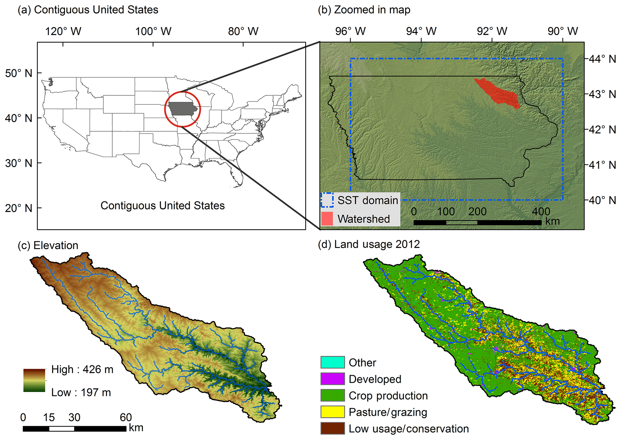
Figure 1Study region. (a) Contiguous United States with the state of Iowa highlighted in grey. (b) Zoomed-in map showing Iowa (black outline) and the Turkey River watershed (red) and the extent of the stochastic storm transposition region (blue dashed line). (c, d) The Turkey River watershed showing land surface elevation (based on the USGS National Elevation Dataset) and land use (based on the USGS 2012 NLCD), respectively.
We use daily discharge observations for 84 years (1933–2016) from the USGS streamgage at Garber to understand the hydroclimatology of flooding and to validate our FFA results. Daily discharge observations for 69 years (1948–2016), in conjunction with Global Historical Climate Network (GHCN) daily temperature and snow data, are used to configure, calibrate, and validate the hydrologic model, as described in Sect. 4.1. CPC US Unified (CPC-Unified; Chen et al., 2008) and Stage IV (Lin and Mitchell, 2005) precipitation data, available through the National Oceanic and Atmospheric Administration, are used for rainfall analyses. CPC-Unified provides daily, 0.25∘ rainfall estimates interpolated from rain gage observations, while Stage IV provides hourly, approximately 4 km estimates by merging data from rain gages and the National Weather Service Next-Generation Radar network (NEXRAD; Crum and Alberty, 1993). Analyses based on Stage IV use data from 2002 to 2016, while long-term analyses based on CPC-Unified use data from 1948 to 2016.
The FFA approach presented in this study combines continuous simulation (CS), stochastic storm transposition (SST) using the RainyDay software, and event-based simulation. CS provides large samples of seasonally varying antecedent conditions, namely, soil moisture and snowpack. SST produces large numbers of synthetic rainfall scenarios. Together, these drive event-based simulations to generate the synthetic flood peaks that are used to derive flood frequency distributions. The approach is illustrated schematically in Fig. 2 and summarized in the following subsections.
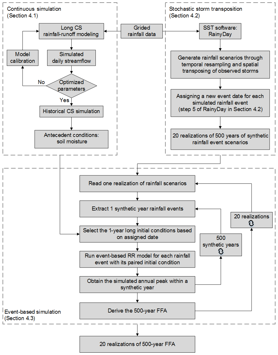
Figure 2Flowchart showing the process-based FFA approach. Dotted outlines delineate components associated with Sects. 4.1, 4.2, and 4.3.
4.1 Hydrologic model, calibration, and continuous simulation
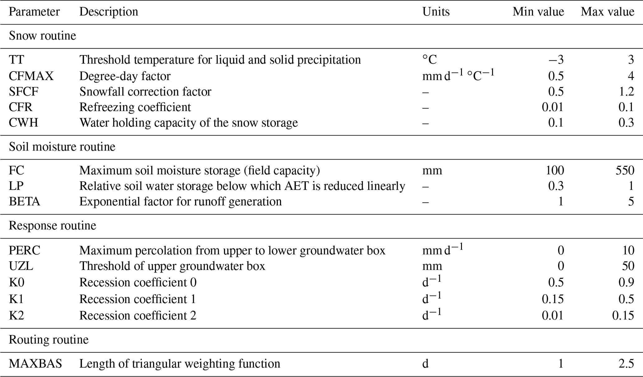
We used the lumped Hydrologiska Byråns Vattenavdelning (HBV) model (Bergström, 1992, 1995; Lindström et al., 1997). HBV has been widely used to study hydrologic response in the United States (Vis et al., 2015; Niemeyer et al., 2017) and other regions of the world (Harlin and Kung, 1992; Osuch et al., 2015; Seibert, 2003; Chen et al., 2012). The “HBV-Light” version (henceforth referred to as HBV; Seibert and Vis, 2012) used in this study consists of four main routines: the snowpack, soil moisture, catchment response, and runoff routines. HBV simulates daily discharges based on time series of precipitation and air temperature, as well as estimates of long-term daily potential evapotranspiration. A list of model parameters is shown in Table 1.
Table 1Overview of HBV model parameters and upper and lower parameter limits used for calibration.
The process-based FFA methodology employed in this study could be coupled with other hydrologic models. A distributed model would allow for more realistic representation of important characteristics like changing land use, rainfall spatiotemporal structure, and flood wave attenuation in river channels, and could operate at higher (i.e., subdaily) temporal resolution. We selected HBV at the daily time step due to its simplicity, its computational speed, and its ability to represent multiple watershed hydrological processes.
We calibrated separate HBV models using both CPC and Stage IV rainfall. Most parameter values were the same for CPC- and Stage IV-based models, except for three snow routine parameters (TT, CFMAX, SFCF) and three recession coefficients (K0, K1, K2), allowing for the variability of model parameters for different climate conditions. For each model setup, we first calibrated the model with the snowpack routine “turned off” (by setting the TT parameter to a very low value) to obtain parameters that can simulate summer floods adequately. Then, keeping these optimized non-snow routine parameters unchanged, we calibrated the snow routine parameters.
To determine the optimized model parameter sets in each procedure, we followed the Genetic Algorithm and Powell (GAP) optimization method as presented by Seibert (2000), which is briefly summarized here. First, 5000 parameter sets are randomly generated from a uniform distribution of the values of each parameter (Table 1), which were then applied to the HBV model in order to maximize the Kling–Gupta efficiency (Gupta et al., 2009) of simulated daily discharge. After the GAP has finished, the optimized parameter sets were fine-tuned using Powell's quadratic convergent method (Press, 1996) with 1000 additional runs. Lastly, the optimized parameter set was manually adjusted to improve the fits between observed and simulated annual peak flow (see Lamb, 1999). More elaborate calibration and uncertainty estimation procedures such as generalized likelihood uncertainty estimation (GLUE; Beven and Binley, 1992, 2014; Beven, 1993) could be used, but are outside the scope of our study.
The two different HBV models were then used to perform CS with historical CPC and Stage IV rainfall and temperature data to derive long-term simulated soil moisture and snowpack values, which are usually difficult to obtain via measurement. We “pair” samples of these initial conditions with synthetic rainfall events to simulate hypothetical floods, as described in Sects. 4.2 and 4.3.
4.2 Stochastic storm transposition
Stochastic storm transposition (SST) is a bootstrap method to generate realistic probabilistic rainfall scenarios through temporal resampling and spatial transposing of observed storms from the surrounding region. SST effectively “lengthens” the rainfall record via “space-for-time substitution”. Unlike rainfall IDF curves, SST can preserve observed rainfall space–time structure, and, unlike design storm methods, obviates the need to equate rainfall duration with catchment response time (Wright et al., 2013, 2014a, b). Alexander (1963), Foufoula-Georgiou (1989), and Fontaine and Potter (1989) provide general descriptions of SST. Wilson and Foufoula-Georgiou (1990) apply the method for regional rainfall frequency analysis, while Gupta (1972), Franchini et al. (1996), England et al. (2014), and Nathan et al. (2016) use it for FFA.
Wright et al. (2013) used SST with a 10-year high-resolution radar rainfall dataset to estimate spatial IDF relationships. Wright et al. (2014a) used this approach with a physics-based distributed hydrologic model for FFA in a heavily urbanized watershed, demonstrating its usefulness in evaluating multi-scale flood response.
RainyDay is open-source, Python-based SST software that couples SST methods with rainfall remote sensing data. A more detailed description can be found in Wright et al. (2017); not all of its features are used in this study. The following steps describe how RainyDay is used here.
We define a 6∘ (longitude) by 4∘ (latitude) geographic transposition domain (40 to 44∘ N, 90 to 96∘ W; blue dashed line of Fig. 1 inset) which encompasses the Turkey River watershed. This same domain was used in Wright et al. (2017) and, importantly for the SST approach, extreme rainfall properties are roughly homogeneous within it.
The RainyDay software creates a “storm catalog” from 15 years of Stage IV (69 years of CPC) precipitation data that consists of the 450 (2070) most intense precipitation events within the transposition domain. These intense storms are in terms of 96 h rainfall accumulation and have the same size, shape, and orientation of the Turkey River watershed, which is oriented roughly northwest–southeast and with an area of 4002 km2. In order to avoid overlapping storms, these selected events must be separated by at least 24 h. Storms that exhibit “radar artifacts” such as major bright band contamination or beam blockage are excluded from subsequent steps.
The RainyDay software generates a Poisson-distributed integer k that represents a “number of storms per year”. The rate parameter λ of this Poisson distribution is calculated by dividing the total number of rainfall events in the storm catalog by the number of years in the historical rainfall record (e.g., storms per year).
RainyDay randomly selects k storms from the storm catalog and transposes the associated rainfall fields within the transposition domain by an east–west distance Δx and a north–south distance Δy, where Δx and Δy are drawn from a two-dimensional Gaussian kernel density estimate based on the locations of the original storms in the storm catalog. For each of the k-transposed storms, the time series of rainfall over the Turkey River watershed is computed. It must be noted that some of the k-transposed storms may not “hit” the Turkey River watershed, and thus their calculated watershed rainfall is zero. Steps 3 and 4 can be understood as temporal resampling of observed rainfall events to “synthesize” a hypothetical year of rainfall events over the transposition domain and, by extension, over the watershed. Although the rainfall events for the “synthetic” year do not form a continuous series, the dates associated with each observed storm event are recorded, thus facilitating seasonally consistent flood simulations.
All k events within a synthetic year are assigned a new, randomly selected year from 1948 to 2016 (2002–2016) for CPC (Stage IV) rainfall data which used to select antecedent conditions. This ensures that the k rainfall events are all “embedded” within a single realistic annual representation of watershed conditions. This ensures that “wet” and “dry” years in terms of snowpack and soil moisture can potentially produce wet or dry years of flood response. Antecedent conditions are randomly selected from within 7 days of the updated storm date to ensure realistic seasonality of storms and watershed conditions. A storm that occurred on 15 July 2016, for example, could be paired with initial conditions selected from a date ranging between 8 and 22 July from a randomly selected year, while the remaining k−1 events would be paired with seasonally appropriate initial conditions from the same selected year.
RainyDay repeats Steps 3–5 500 times to create one realization of 500 synthetic years of rainfall events for the Turkey River. Twenty such realizations of 500 synthetic years each are generated. Unlike in the existing version of RainyDay, all rainfall events within a synthetic year are retained for subsequent event-based flood simulations, since the modulating effects of antecedent conditions mean that the largest rainfall event in a given year does not necessarily produce that year's largest flood peak (this is explored in Sect. 5.4).
4.3 Event-based flood simulation
Using the seasonally consistent “paired” watershed initial conditions derived from CS (Sect. 4.1) and SST-based rainfall events (Sect. 4.2), HBV simulates the “event peak” (the maximum daily discharge). The largest peak among the k events that comprise a synthetic year represents the simulated annual maximum daily streamflow. As mentioned in Step 5 of the SST procedure (Sect. 4.2), each synthetic rainfall event is randomly paired with seasonally appropriate initial conditions (soil moisture, snowpack) and air temperature drawn from the continuous simulation (15 years in the case of Stage IV; 69 years for CPC). This creates combinations of initial conditions and forcing that in principle reflect the true variability of these processes. This procedure is repeated for all 500 synthetic years within each realization, resulting in 500 annual maximum streamflow values, which are then ranked in descending magnitude. The annual exceedance probability pe (i.e., the probability in a given year that an event of equal or greater magnitude will occur) of each maximum streamflow is calculated by dividing its rank by 500 (the total number of simulated annual maximum daily streamflow). The 20 realizations provide estimates of variability for each flood quantile.
5.1 Hydroclimatology and nonstationarity
Four distinct time periods (Fig. 3a) are considered for analyzing the changing hydroclimatology in the Turkey River: the USGS daily mean streamflow period of record (1933–2016), a more recent period of apparent elevated flood activity (1990–2016), the period of the Stage IV rainfall record (2002–2016), and the period of the CPC rainfall record (1948–2016). Results here and in subsequent subsections “align” with one or more of these time periods.
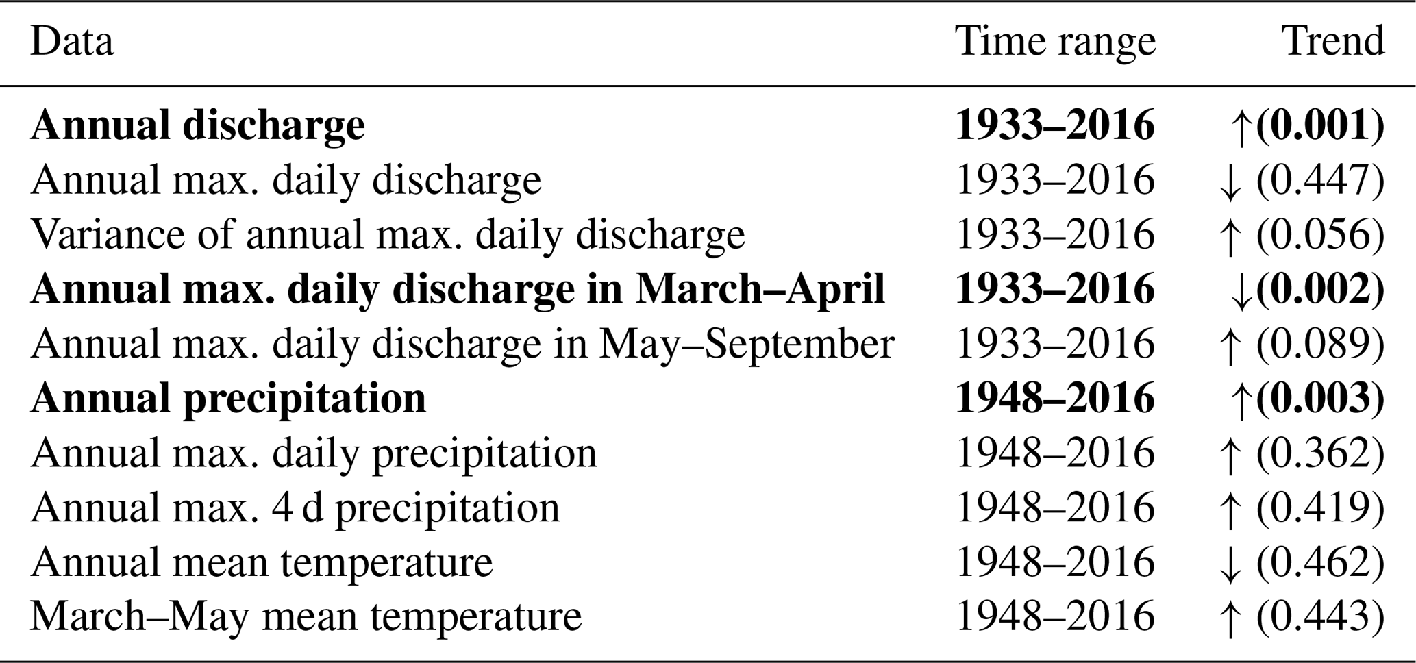
The hydroclimate of the Turkey River is changing, as shown using the Mann–Kendall (MK) test for monotonic trends (Mann, 1945), a nonparametric method used to determine trend direction and significance (Table 2). Since 1948, annual precipitation and discharge have shown significant increases (p<0.05) and their variability has also increased, while annual maximum daily discharge has decreased, though not significantly. It is important to note, however, that there are two counteracting seasonal trends (see also Fig. 3a): annual daily discharge maxima have decreased significantly in March–April, but have increased somewhat in May–September. Thus, the lack of statistically significant change in annual maximum daily discharge in the Turkey River masks changes in the seasonality of flooding.
Table 2Mann–Kendall trend test (two-sided) for hydrological variables. p-values are given in parentheses; bold values are significant at the 5 % level. Analyses of trends in variances examine changes in the absolute values of residuals obtained from a linear regression using the Thiel–Sen estimator (Sen, 1968).
We examine this flood seasonality, both in observations and in our continuous HBV simulations (Fig. 3b). The seasonal distribution of flood occurrence for 1948–2016 shows a March–April maximum, with elevated flood activity continuing through May and June. This is distinct from though overlaps somewhat with the seasonality of both the 4-day annual maxima of rainfall, which occur most frequently in the June–September period, and simulated daily annual maxima soil moisture, which only tends to occur in March–April. These results highlight that flood activity is the product of seasonal variations in both soil moisture and rainfall. (Four-day rainfall shown in Fig. 3b since it is used in SST; seasonality in 1-day rainfall is similar; results not shown).
The March–April peak of flood occurrence corresponds to relatively high soil moisture associated with snowmelt, rain on or frozen soil, and frequent spring rains. The secondary peak of flood occurrence in May–June is associated with larger flood magnitudes (including the flood of record, in 2004) due to organized thunderstorm systems. Widespread flooding in Iowa in June 2008 showed that such thunderstorm systems make critical contributions to the upper tail of flood peak distributions in the region (Smith et al., 2013). Although the frequent August–September heavy rainfall events evident in Fig. 3b have not triggered any recorded annual flood peaks in the Turkey River, our process-based FFA demonstrates that they may still be relevant to current and future flood frequency, as shown in Sect. 5.4.
The largest annual maxima (over 800 m3 s−1) occur in May–July (Fig. 3c), consistent with the broader climatology of flooding in Iowa (Smith et al., 2013; Villarini et al., 2011). Furthermore, both the seasonality and magnitude of flood peaks have shifted since approximately 1990 (Fig. 3a, c), with March–April (May–September) floods decreasing (increasing) in magnitude, leading to a shift in the seasonality of the overall distribution of annual maximum daily streamflow from a high in March prior to 1990 to a prolonged high from April to June post-1990. Although the small sample size of the annual maximum daily discharge during this elevated 1990–2016 late-spring and summertime flood period may affect the reliability of the derived distribution of flood occurrence, Park and Markus (2014) also reported a significant shift toward summertime flooding in the nearby Pecatonica River. Statistically based FFA (including nonstationary methods) based on annual maxima discharges may fail to capture the impact of this shifting seasonality on flood frequency.
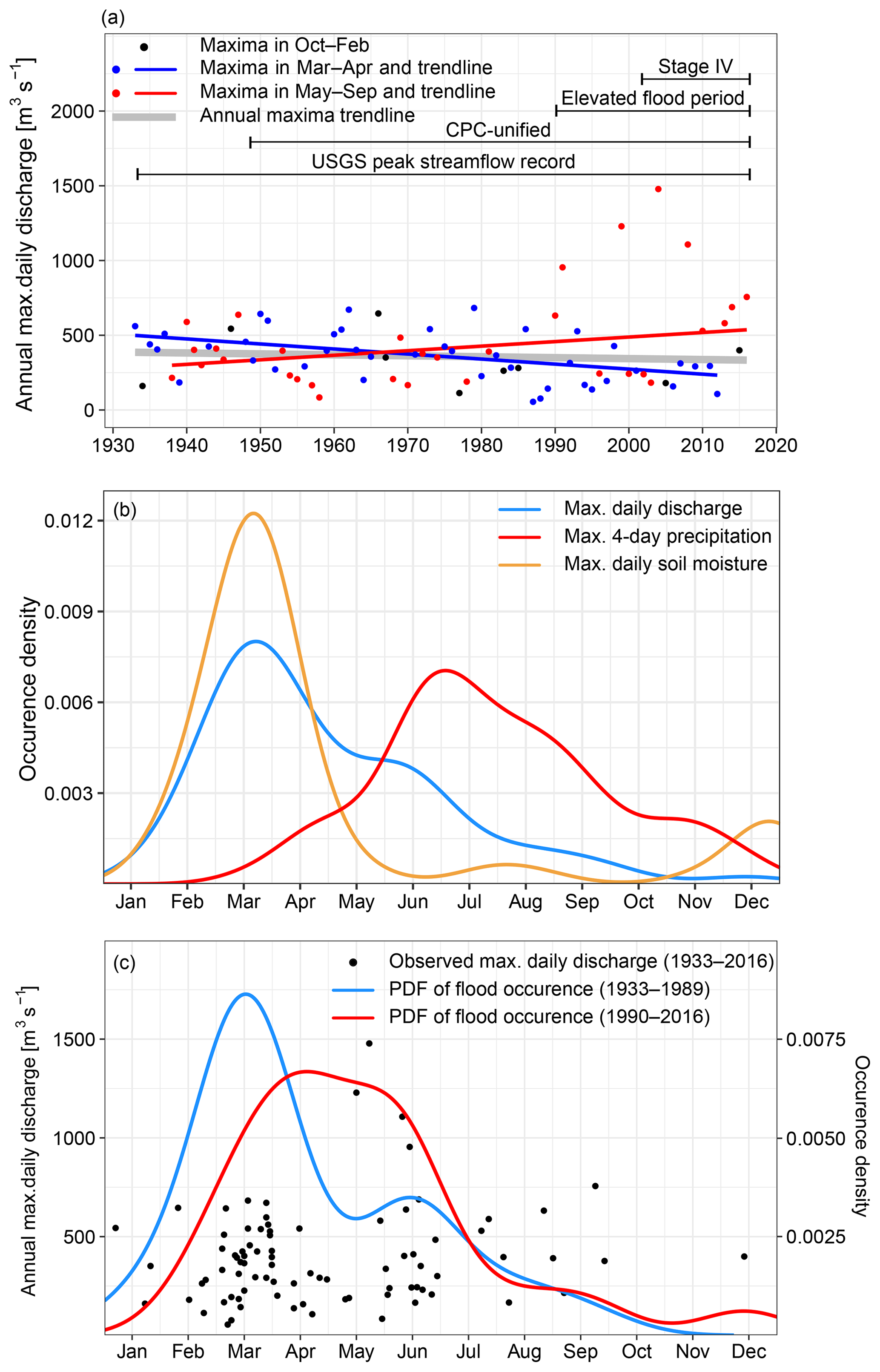
Figure 3(a) Linear trends for two groups of annual maximum daily discharge: March–April floods (blue) and May–September floods (red) using the nonparametric Thiel–Sen estimator (Sen, 1968). The October–February maximum daily discharges are in black dots and their trend line is not calculated because only nine annual maxima occur during this period. The four critical time ranges are shown in black lines. (b) Occurrence densities of the date during the year for the observed annual daily maximum discharge, observed annual 4 d maximum precipitation, and simulated annual daily maximum soil moisture in the Turkey River watershed from 1948 to 2016. (c) The magnitude and date during the year for annual flood peaks (black dots) and sample probability density functions (PDFs) for floods in different periods (1933–1989, 1990–2016). In this study, all probability densities for the occurrence date are estimated using Gaussian kernel smoothing.
5.2 Model validation
We validated the performance of continuous HBV simulations with respect to flood seasonality, frequency of annual daily discharge maxima, and normalized peak flow (i.e., the simulated or observed daily discharge divided by the 2-year flood), using both Stage IV and CPC as precipitation inputs (Fig. 4). We also validated two model structures: one with and the other without the HBV snowpack module. The purpose of this latter validation effort is to highlight the importance of proper process representation (and subsequent validation) in process-based FFA.
Simulated flood seasonality varies substantially during the CPC period of record (1948–2016) depending on the inclusion of the snowpack routine (Fig. 4a). Differences are less for the Stage IV period of record (2002–2016), due to the decreasing role of snowpack in deriving the floods in recent years (Fig. 4b). In both cases, the seasonality of flooding simulated using HBV is improved with the inclusion of the snowpack module, with a higher (lower) frequency of springtime (summertime) floods which more closely resembles observations. Empirical (i.e., plotting position-based) distributions for the simulated annual daily discharge maxima are mostly within the 90 % confidence interval (obtained by nonparametric bootstrap) of the observations (Fig. 4c, d). CPC-based simulation results differ considerably depending on the inclusion of the snowpack module for more common events, but differences in simulated maxima vanish as flood magnitude increases (e.g., AEP < 0.1). This is because the most extreme flood events occur later in the season and are thus independent of snowpack or snowmelt processes. Differences are generally negligible between Stage IV-based simulations with and without snowpack, since floods in this more recent period are generally driven by summertime thunderstorms. These findings are consistent with the general understanding of the regional seasonality of flooding in the region, as discussed in Sect. 5.1.
We compared all simulated and observed flood peaks that can be associated with a USGS-observed daily streamflow value that is at least 3 times the mean annual daily discharge (Fig. 4e, f). When associating simulated and observed flood peaks, we look within a 2 d window to allow for modest errors in simulated flood peak timing. All peaks in Fig. 4e and f are normalized by the median annual (i.e., 2-year) flood, which, as a rule of thumb, can be considered the “within-bank” threshold. Again, HBV with the snowpack routine outperforms the model without it, especially for the small to modest flood events in CPC-based simulations. The model without snowpack underestimates small to modest flood events in two cases due to the neglect of potential snowmelt contributions. While modest scatter exists in the Stage IV-based simulated peaks, there is no obvious systematic bias with event magnitude when the snowmelt routine is included. The good performance of the Stage IV simulations suggests that, when focusing on the recent period of elevated flood activity, Stage IV may be a more suitable rainfall input than CPC-Unified. In addition, CPC rainfall is known to contain errors in the extreme tail, due to gage “undercatch”, insufficient gage density to properly sample convective rain cells, and spatial averaging of such cells over large areas, which effectively reduces peak rainfall depths.
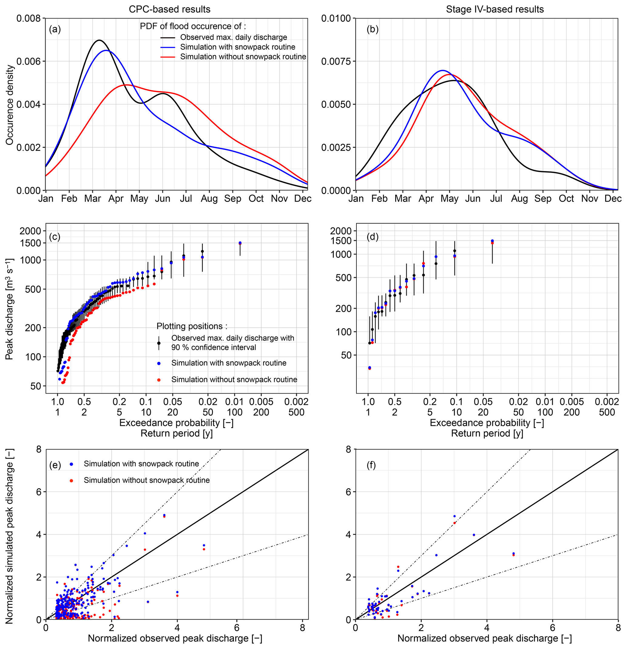
Figure 4HBV model validation for flood seasonality (a, b), frequency of annual maximum daily discharge (c, d), and normalized peak flow (e, f) for CPC and Stage IV-based continuous simulations. Model validation is performed for HBV simulations with and without using CPC for 1948–2016 (a, c, e) and Stage IV for 2002–2016 (b, d, f). The 90 % confidence intervals for the empirical distributions of observed maximum daily discharges (c, d) are derived using nonparametric bootstrapping. Flood peak discharge in (e) and (f) is defined as a data point with an USGS-observed value that is at least 3 times the average observations. Peak discharges are normalized by the median of annual daily discharge maxima (i.e., the 2-year flood). Straight solid black lines indicate 1:1 correspondence, while dashed lines denote an envelope within which the modeled values are within 50 % of those observed.
We also validate HBV's snowpack routine using observed GHCN daily snow depth for two simulation periods (Fig. 5a, b) and using USGS daily streamflow observations for a Stage IV-based period (Fig. 5c). Because of their differing spatial resolutions and physical representations, point-scale GHCN daily snow depths cannot be directly compared to the watershed-scale snow water equivalent simulated by HBV. Instead, we validate snowpack simulations in terms of the snowpack occurrence, defined as the number of nonzero snowpack on a particular date divided by the total number of years in the historical or simulated record. For example, there are 50 d in the GHCN observations when snowpack is present on 1 January in the 69-year period from 1948 to 2016; thus, the occurrence rate is 0.72 (50 divided by 69). The HBV model with the snowpack routine captures the central tendency of observed snowpack dynamics, showing that snowpack frequently exists from early November to mid-February, with frequency of snow decreasing from late February until disappearing in early April.

Figure 5Percentage of days with nonzero snowpack present in observations and simulations (a, b) and hydrograph validation for Stage IV-based simulation (c). For each day within a year, the percent with nonzero snowpack is calculated as the ratio of the number of years in which snowpack is present on that day to the total years (69 years for CPC and 15 years for Stage IV). Observed and simulated hydrographs are normalized by the median annual flood, which is indicated by the dashed blue line.
Model hydrograph validation is provided in Fig. 5c for the Stage IV period (2002–2016), when major flooding occurred throughout Iowa. Model performance shows no obvious evidence of systematic bias in the streamflow simulations (see also Fig. 4f). Although flood seasonality derived from Stage IV-based simulation differs slightly from observations (see also Fig. 4a), these mismatches are associated with flood events smaller than the median annual flood (blue dashed line in Fig. 5c). Stage IV-based simulations do not show bias flood magnitude in late summer. In other words, remaining biases in terms of flood seasonality generally correspond to frequent, small-magnitude events that are typically of less interest in FFA. We therefore conclude that the HBV model with snowpack is generally suitable for subsequent process-based FFA.
5.3 Flood frequency analyses
RainyDay-based flood frequency distributions for the Turkey River at Garber using both Stage IV and CPC precipitation are compared with the distribution based on statistical analyses of discharge observations using 1933–2016 USGS annual maximum daily streamflows (Fig. 6). The latter is estimated using the HEC-SSP software (Bartles et al., 2016), which implements methods from Bulletin 17B (Interagency Advisory Committee on Water Data, 1982) using “station skew” to fit the log-Pearson Type III distribution. Observed annual daily streamflow maxima from 1933 to 2016 are also shown, where plotting position (pe) is estimated using the Cunnane plotting position (Cunnane, 1978). As mentioned above, different HBV parameters are used for the Stage IV and CPC-based simulations; this is necessary due to the differing time periods and error properties of these two precipitation datasets.
The Stage IV-based flood frequency curve agrees reasonably well with the Bulletin 17B results for pe>0.3 ( panel (a) of Fig. 6), but yields higher estimates for rarer events. The CPC-based curve, on the other hand, matches closely with Bulletin 17B. The Stage IV analyses use shorter but more recent (2002–2016) meteorological and hydrological records than the other frequency curves. When streamflow observations are divided into two groups (1933–1989 and 1990–2016), it becomes clear that the recent peak flood observations align well with the Stage IV-based SST results (panel (b) of Fig. 6). This, along with the increasing trend of annual mean precipitation and discharge shown in the previous subsection, suggests that, despite the relatively short (15-year) rainfall record used, Stage IV-driven process-based FFA adequately reflects flood frequency in the wetter recent climate (a similar result is shown in Wright et al., 2017), while the CPC-based and Bulletin 17B methods, both based on much longer data records, fail to do so.
The results shown in Fig. 6 suggest that the recent shift from spring to summer flood activity is accompanied by a substantial shift in the flood frequency distribution. The close agreement between process-based results using CPC and the statistically based analysis using Bulletin 17B suggests that even in stationary situations with long records, statistical methods do not necessarily produce superior results to process-based approaches. Process-based FFA using CPC precipitation from 2002 to 2016 closely resembles the Stage IV-based FFA (results not shown), suggesting that rainfall process nonstationarity, rather than differences between different input datasets, is the primary driver of the differences in the CPC-based and Stage IV-based results in panel (a) of Fig. 6.
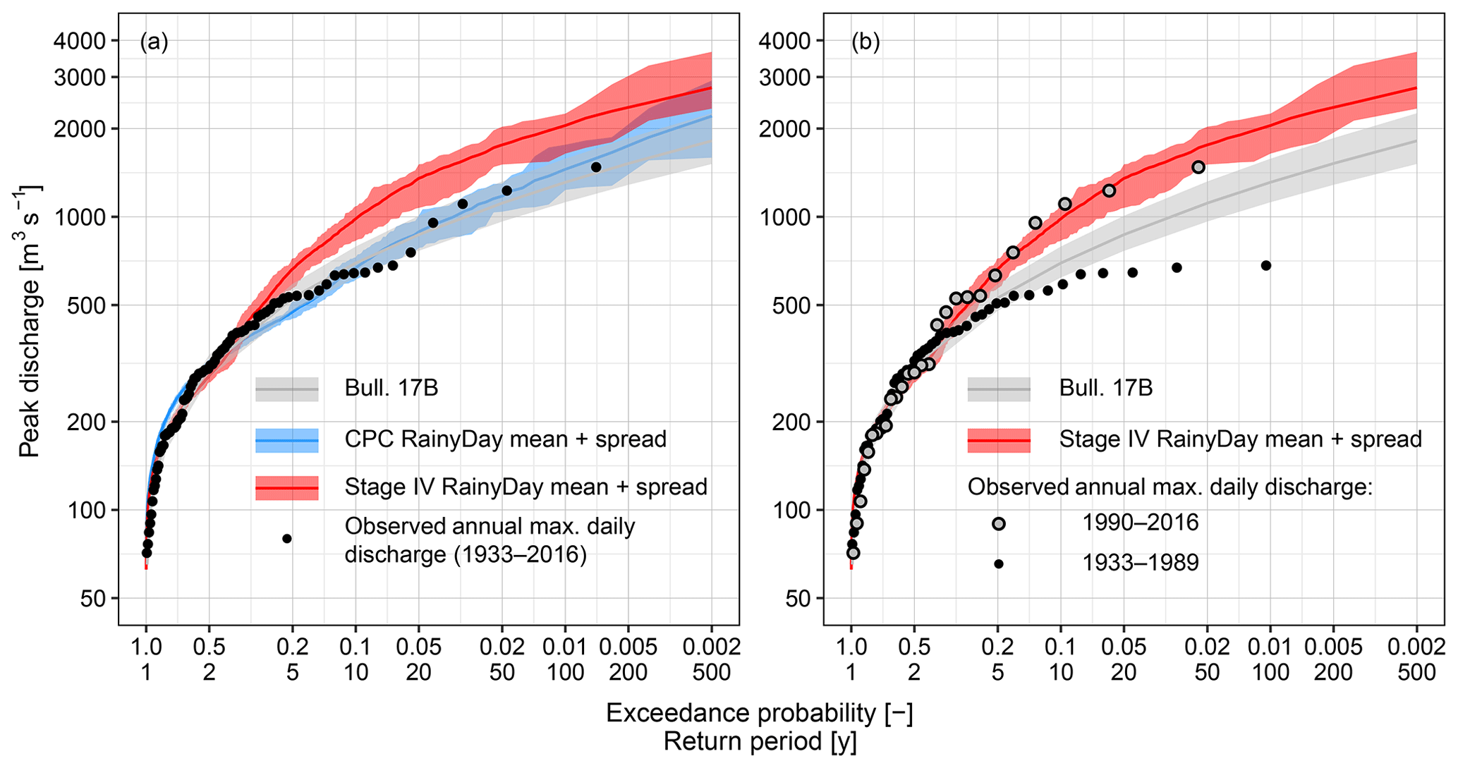
Figure 6Peak discharge analyses for the Turkey River at Garber, IA. (a) RainyDay with Stage IV (2002–2016) and CPC (1948–2016) rainfall and USGS frequency analyses using Bulletin 17B methods. All observed USGS annual maximum daily streamflows from 1933 to 2016 are also shown. Shaded areas denote the ensemble spread (RainyDay-based results) and the 90 % confidence intervals (Bulletin 17B-based analysis), respectively. (b) Same as (a), but with the USGS observations divided into pre-1990 and post-1990 groups, and replotted to highlight recent changes in flood frequency.
5.4 Simulated flood seasonality
As shown in Sect. 5.1, the recent climatology of flooding in the Turkey River watershed shows a peak in flood occurrence during March–April, with elevated activity (including high-magnitude events) continuing through July, reflective of the regional flood “mixture distribution” (e.g., Smith et al., 2011). March–April flooding is associated with springtime rains, high soil moisture, and potentially snowmelt processes, while May–July flooding results from warm-season organized thunderstorm systems. It is important that any process-based FFA approach capture the influence of this mixture on the flood frequency curve.
The seasonal distribution of simulated flood occurrence and magnitude using Stage IV- and CPC-based results shows that most simulated floods in our process-based approach occur between March and June (Fig. 7), in accordance with observed annual maximum daily discharge (Fig. 3c). The peak of occurrence using Stage IV is shifted several weeks later than the CPC-based results, which agrees with the recent shift in seasonality of flood observations shown in Fig. 3c. Although many simulated events still occur in April, our results show the largest peaks occur later, in May–September. This is consistent with Villarini et al. (2011), who showed that warm-season organized convective systems are responsible for some of the largest peaks in Iowa.
Our process-based results show that August–September storms have the potential to cause severe flooding (Fig. 7), despite the lack of large floods during this time of year in the stream gage record. Stage IV- and CPC-based storm catalogs generated by RainyDay include major storms from the surrounding region, including several large late-summer events capable of producing substantial flood response, and which indeed induce large floods within our process-based analysis. This suggests that the general lack of major late-summer floods in the watershed's observational record may not be a feature of the “true” (unknown) distribution of flooding in the watershed, but is rather due to limited size of the observational record. This result is supported by regional analysis of floods (Villarini et al., 2011) and points to the potential for SST to improve understanding of flood frequency seasonality relative to discharge-based approaches alone.
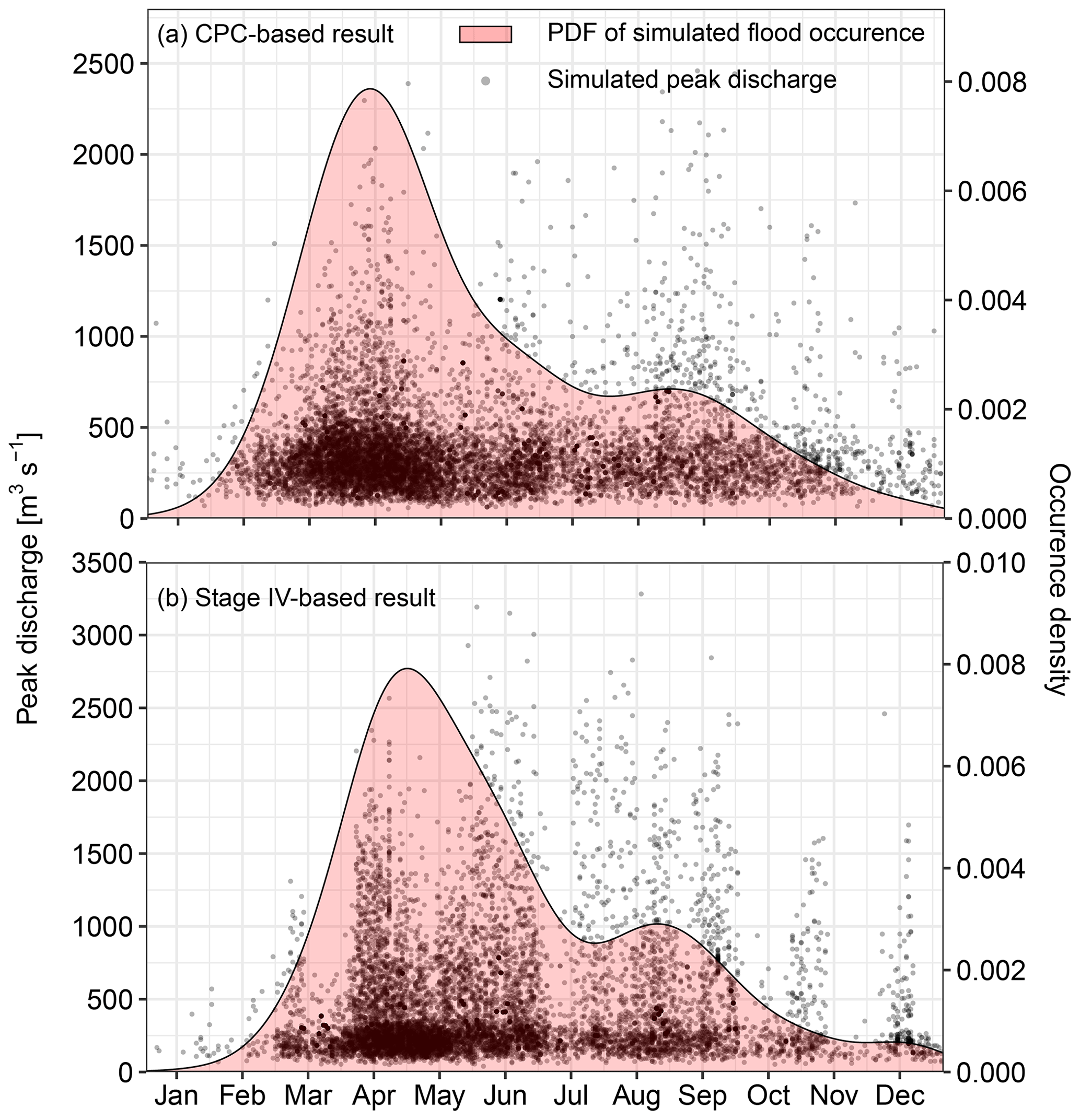
Figure 7Time of occurrence during the year for simulated peak discharge in the Turkey River at Garber using (a) CPC and (b) Stage IV.

Figure 8The simulated flood magnitude using CPC rainfall during the 1948–2016 (a) and 2002–2016 (b) periods, and corresponding antecedent conditions. The blue triangles denote the snow-related flood events (e.g., snowmelt was nonzero in the simulation) and grey dots represent the non-snow-related flood events (e.g., rainfall driven). The sizes of the triangles or dots indicate the antecedent soil moisture with a higher value in a larger shape. The black dashed line indicates the 1000 m3 s−1 flood magnitudes.
To demonstrate that the discrepancies between the process-based FFA results generated using CPC and using Stage IV are driven by changes in physical processes, rather than by differences in model structure (i.e., parameter values), we compared FFA results generated using CPC-based simulation for 1948–2016 and 2002–2016, in terms of event rainfall, initial soil moisture, flood type, and peak magnitude (Fig. 8). Compared with the 1948–2016 period (Fig. 8a), there are fewer flood events driven by snowmelt or rain-on-snow during 2002–2016 (Fig. 8b), but more driven by rainfall. This is particularly true for flood events (larger than 1000 m3 s−1). In addition, some of the rainfall-driven floods from 2002 to 2016 were caused by relatively low rainfall but high initial soil moisture, in accordance with the significant increasing trend of annual precipitation and discharge (Table 2).
5.5 Comparison of rainfall and peak discharge quantiles
We examined the relationships between the return periods of 96 h basin-averaged rainfall accumulations and simulated peak discharge for the Turkey River at Garber using Stage IV-based results (Fig. 9; CPC-based results show similar patterns and thus are not shown here). Antecedent soil moisture for each simulated event is also shown. Similar to Wright et al. (2014a), Fig. 9 shows that simulated peak discharge quantiles can differ substantially from the rainfall quantiles of the rainfall that produces them. For instance, 500-year (pe=0.002) rainfall events can cause simulated peak discharges ranging from 11 years (pe=0.091) to 500 years (pe=0.002), corresponding to a range in peak discharge of 1072 to 2743 m3 s−1. Peak discharge quantiles are always larger (in terms of return period) than the quantiles of rainfall that produced them in wet antecedent soil moisture conditions, while the reverse is true in for dry conditions. These results also demonstrate that the DS assumption of 1:1 equivalency between rainfall and peak discharge quantiles does not hold in the Turkey River. Rainfall spatial variability and drainage network structure, which are ignored in this study due to the lumped (i.e., non-distributed) nature of HBV, further complicate the relationship between rainfall and discharge quantiles.
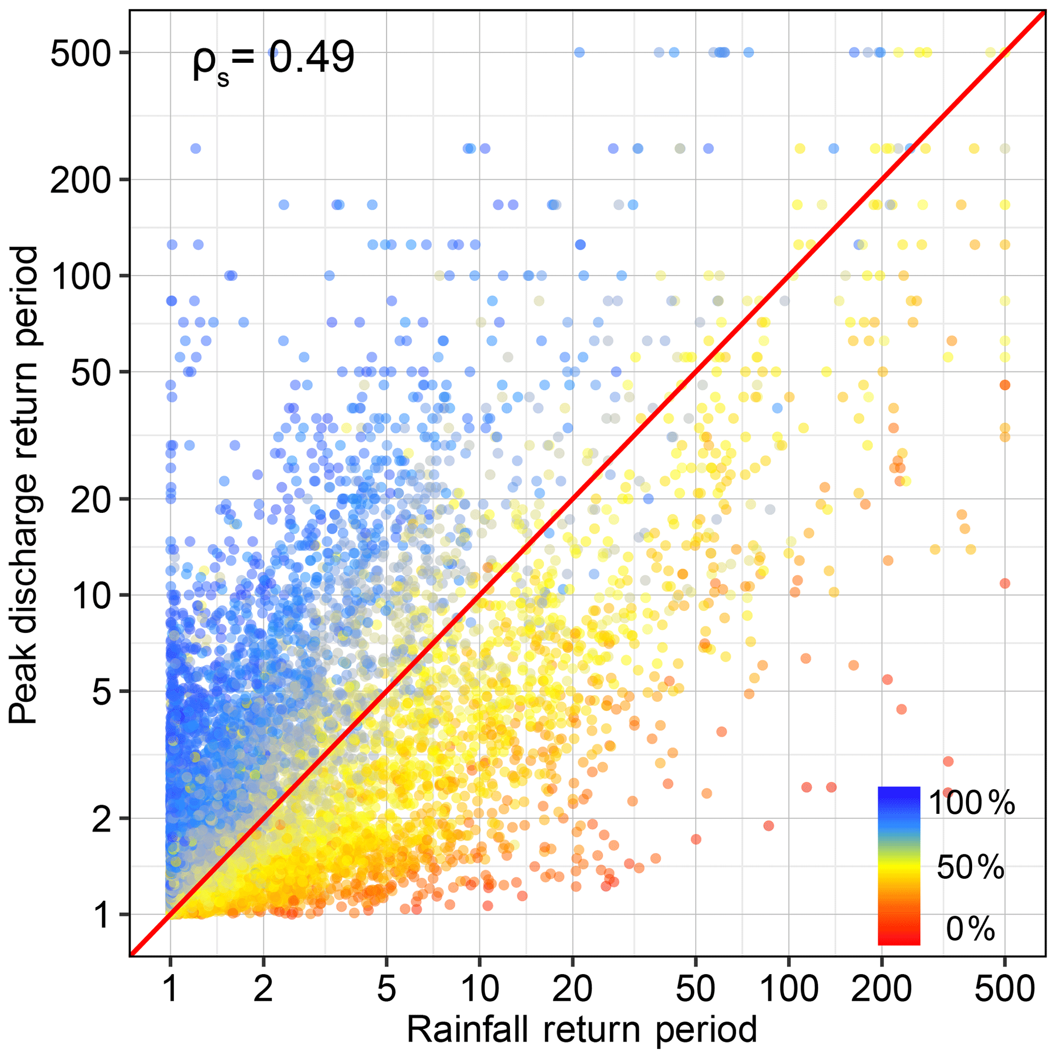
Figure 9Relationships between rainfall and simulated peak discharge return periods estimated via our process-based method using Stage IV rainfall data. Spearman rank correlation ρs is given. Color indicates the normalized modeled antecedent soil moisture value calculated as %.
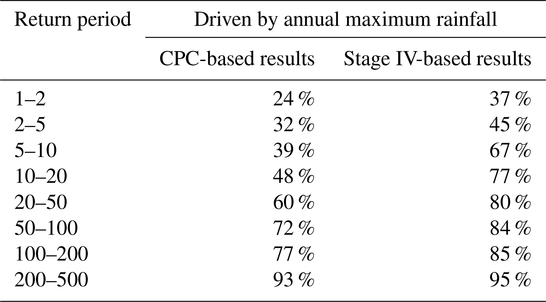
We further examine the relationship between annual rainfall and annual flood peak maxima. In Sect. 2.2, we pointed out that DS methods utilize IDF curves, which are usually estimated using annual maxima from rain gage records and which depict quantiles from the distribution of annual rainfall maxima. DS methods use quantiles from this distribution to generate flood estimates, implicitly assuming that annual rainfall maxima produce annual discharge maxima. In our process-based FFA approach, we do not assume that annual discharge maxima are the result of the largest rainfall event of the year. Rather, lower-magnitude rainfall events, combined with high soil moisture, could produce the highest discharge. Table 3 shows the percentage of annual peak flow driven by annual maximum gains with increasing return periods for both CPC-based and Stage IV-based results. For simulated peak flow with pe>0.01, a large portion of simulated annual peak flow is not caused by the annual maximum rainfall. For rarer peak flows (pe≤0.01), over 90 % of these flood events are driven by the annual maximum rainfall, pointing to the fact that the tail of flood peaks is driven by extreme rainfall, with antecedent conditions playing a modulating role.
Table 3Percentages of simulated annual maximum daily flows driven by 96 h rainfall annual maximum.
Interactions between rainfall, land cover, river channel morphology, and watershed antecedent conditions are important drivers of flood response. Standard approaches to estimate extreme flood quantiles (termed flood frequency analysis; FFA), however, often take a superficial view of these interactions, as argued in Sect. 2. This study presents an alternative FFA framework that combines elements of observational analysis, stochastic rainfall generation, and continuous and event-scale hydrologic simulation. We apply the framework to the Turkey River, an agricultural watershed in the Midwestern United States that is undergoing significant hydroclimatologic and hydrologic change which is increasing the magnitude of the largest flood events and shifting their occurrence from the spring to summer.
We use stochastic storm transposition (SST) to create and resample from “storm catalogs” developed from both 15 years of high-resolution bias-corrected radar rainfall and from 69 years of gridded rain gage observations to produce large numbers of rainfall scenarios for the Turkey River. These scenarios, when coupled with seasonally realistic watershed conditions, can help to reconstruct the seasonal and secular variations in meteorological and hydrological processes and their interactions, providing an alternative FFA approach which is well-suited to nonstationary environments (see also Sivapalan and Samuel, 2009). While statistical approaches can in principle be applied to investigate the impacts of seasonality on FFA (e.g., Ouarda et al., 2006), such methods still do not directly provide process-level understanding of the factors that “shape” flood frequency. Unlike design storm approaches to FFA, the synthetic rainfall scenarios derived by the SST-based procedure do not require any assumptions regarding the spatial and temporal structure of rainfall, since they are driven by the structure and variability of historical observed storms.
Our analyses show that using the most recent 15 years of rainfall can produce realistic “present-day” flood quantile estimates that reflect the nonstationarities in rainfall and watershed conditions. The use of longer records, within both our procedure and conventional statistical FFA methods, leads to underestimates of current flood frequency due to their inability to represent recent shifts in flood activity in the Turkey River. Our results challenge some common FFA assumptions, including the design storm presumption that rainfall annual maxima produce discharge annual maxima and the assumption of 1:1 equivalence in rainfall and flood quantiles. We paint a more complex picture in the Turkey River, in which the shifting seasonality in rainfall and watershed conditions combine to shape the flood frequency. Spatial variability in rainfall structure, soil moisture, land use, and watershed morphology, which are ignored in this study due to the use of a lumped hydrologic model, add further complexity to the flood-generating processes. The proposed framework can be employed with more sophisticated distributed hydrologic models, thus facilitating the examination of rainfall spatial variability and its interactions with other factors (e.g., heterogeneous watershed characteristics and river network processes; Zhu et al., 2018; Viglione et al., 2010a, b). This coupling may prove particularly useful for FFA in large watersheds in which there is a practically infinite number of different combinations of such spatially and temporally varying processes that could produce floods – a population that is almost certain to be undersampled in stream gage records and poorly served by design storm assumptions.
A number of issues remain that make broader usage of our process-based framework challenging. Perhaps the biggest limitation of process-based approaches is the necessity of discharge observations, which are central to both identifying hydrologic changes and to calibrating and validating the hydrologic model. Thus, usage of the approach in ungauged basins may not produce satisfactory results. This issue is fundamental to other FFA techniques as well. Statistically based discharge analyses, for example, similarly rely on streamflow observations, while design storm approaches also require hydrologic model calibration.
We also note that caution is needed when attempting to employ process-based FFA. We were able to produce very similar flood frequency distributions using our approach, regardless of whether or not the HBV hydrologic model's snowpack routine was “turned on” or off (results omitted for brevity), despite very different simulated seasonality of flooding. This highlights that process-based frequency analyses can be influenced by poor model process representation that can lead to seemingly “correct” results for the wrong reasons. This implies that the modeler must have sufficient data and experience to recognize such issues. It also illustrates a key issue in FFA using both statistical approaches and process-based methods: flood quantiles, though the product of interactions between physical processes, reveal relatively little about those underlying processes that produce them. This is particularly problematic in changing hydroclimatic or watershed conditions, because nonstationary behavior is likely the result of seasonal shifts in one or more processes that may affect flooding in ways that are not well-reflected in observational records. Our results showing that major floods could occur in the Turkey River in the late summer under current hydroclimatic conditions, despite their absence in the instrumental record, are one example of this. Failure to recognize and model such shifts could lead to results for past or present flood conditions that appear to be correct but that may lead to incorrect inferences about future conditions.
In summary, our framework and results highlight the opportunity and challenge with process-based FFA approaches, namely, that progress in understanding and estimating flood frequency and how it is evolving in an era of unprecedented changes in land use and climate requires better understanding of how the underlying physical processes, and the interactions between them, are changing. Poor model representation of key hydrological processes, however, can lead to incorrect conclusions about present or future flood frequency. Despite the challenge, we share the view of Sivapalan and Samuel (2009) that process-based approaches hold great potential for advances in FFA research and practice, particularly in projecting future flood hazards in conjunction with data and modeling advances in the climate science community. We do not propose that process-based approaches should necessarily supplant more conventional discharge-based analyses, and acknowledge that discharge observations are essential in such studies. Rather, we anticipate a gradual “merging” of statistical and process-based stochastic simulation techniques as well as of the associated observations and synthetic data.
The RainyDay software is available at Github (https://github.com/danielbwright/RainyDay2, last access: 3 May 2019). A web-based version of RainyDay is available at Daniel B. Wright's research group website (http://her.cee.wisc.edu/projects/rainyday, last access: 3 May 2019, Wright et al., 2017).
The supplement related to this article is available online at: https://doi.org/10.5194/hess-23-2225-2019-supplement.
GY, ZZ and DBW worked together to set up the research goals and to perform the modeling analysis. KDH acquired the financial support for the project leading to this publication and supervised its execution. CS assisted in preprocessing the geospatial data. GY wrote the paper with contributions from all the co-authors.
The authors declare that they have no conflict of interest.
Guo Yu's and Daniel B. Wright's contributions were supported by the U.S. National Science Foundation (NSF) Hydrologic Sciences Program (award number 1749638) and by the Bureau of Reclamation Research and Development Office Project ID 1735, which also supported Kathleen D. Holman's contributions. Cassia Smith's contributions were supported by the U.S. National Aeronautics and Space Administration's MUREP Institutional Research Opportunity. Zhihua Zhu's contributions were supported by Sun Yat-sen University. This study used computing resources and assistance from the UW-Madison Center For High Throughput Computing (CHTC), which is supported by UW-Madison, the Advanced Computing Initiative, the Wisconsin Alumni Research Foundation, the Wisconsin Institutes for Discovery, and the NSF, and is an active member of the Open Science Grid, which is supported by the NSF and the U.S. Department of Energy. We thank Martijn Booij and Marc Vis for their guidance on the HBV model. We would also like to thank the editor and three anonymous reviewers whose constructive comments contributed greatly to the study.
This paper was edited by Matjaz Mikos and reviewed by three anonymous referees.
Alexander, G. N.: Using the probability of storm transposition for estimating the frequency of rare floods, J. Hydrol., 1, 46–57, 1963.
Ayalew, T., Krajewski, W., and Mantilla, R.: Exploring the Effect of Reservoir Storage on Peak Discharge Frequency, J. Hydrol. Eng., 18, 1697–1708, https://doi.org/10.1061/(ASCE)HE.1943-5584.0000721, 2013.
Ayalew, T. B. and Krajewski, W. F.: Effect of River Network Geometry on Flood Frequency: A Tale of Two Watersheds in Iowa, J. Hydrol. Eng., 22, 06017004, https://doi.org/10.1061/(ASCE)HE.1943-5584.0001544, 2017.
Ball, J., Babister, M., Nathan, R., Weeks, W., Weinmann, E., and Retallick, M.: Australian Rainfall and Runoff: A Guide to Flood Estimation, edited by: Testoni, I., Commonwealth of Australia (Geoscience Australia), 2016.
Bartles, M., Brunner, G., Fleming, M., Faber, B., and Slaughter, J.: HEC-SSP Statistical Software Package Version 2.1, Computer Program Documentation, US Army Corps of Engineers, Institute for Water Resources Hydrologic Engineering Center (HEC), 609 Second Street Davis, CA 95616-4687, 2016.
Berghuijs, W. R., Woods, R. A., Hutton, C. J., and Sivapalan, M.: Dominant flood generating mechanisms across the United States: Flood Mechanisms Across the U.S., Geophys. Res. Lett., 43, 4382–4390, https://doi.org/10.1002/2016GL068070, 2016.
Bergström, S.: The HBV Model: Its Structure and Applications, Swedish Meteorological and Hydrological Institute (SMHI), Hydrology, Norrköping, 1992.
Bergström, S.: The HBV model (Chapter 13), in: Computer Models of Watershed Hydrology, edited by: Singh, V. P., 443–476, Water Resources Publications, Highlands Ranch, Colorado, USA, 1995.
Beven, K.: Prophecy, reality and uncertainty in distributed hydrological modelling, Adv. Water Resour., 16, 41–51, https://doi.org/10.1016/0309-1708(93)90028-E, 1993.
Beven, K. and Binley, A.: The future of distributed models: Model calibration and uncertainty prediction, Hydrol. Process., 6, 279–298, https://doi.org/10.1002/hyp.3360060305, 1992.
Beven, K. and Binley, A.: GLUE: 20 years on: GLUE: 20 YEARS ON, Hydrol. Process., 28, 5897–5918, https://doi.org/10.1002/hyp.10082, 2014.
Blazkova, S. and Beven, K.: Flood frequency prediction for data limited catchments in the Czech Republic using a stochastic rainfall model and TOPMODEL, J. Hydrol., 195, 256–278, 1997.
Blazkova, S. and Beven, K.: Flood frequency estimation by continuous simulation for a catchment treated as ungauged (with uncertainty), Water Resour. Res., 38, 14-1–14-14, https://doi.org/10.1029/2001WR000500, 2002.
Blazkova, S. and Beven, K.: A limits of acceptability approach to model evaluation and uncertainty estimation in flood frequency estimation by continuous simulation: Skalka catchment, Czech Republic, Water Resour. Res., 45, W00B16, https://doi.org/10.1029/2007WR006726, 2009.
Calver, A., Lamb, R., and Morris, S. E.: River flood frequency estimation using continuous runoff modelling, Proc. Inst. Civ. Eng.-Water Marit. Energy, 136, 225–234, 1999.
Calver, A., Stewart, E., and Goodsell, G.: Comparative analysis of statistical and catchment modelling approaches to river flood frequency estimation: River flood frequency estimation, J. Flood Risk Manag., 2, 24–31, https://doi.org/10.1111/j.1753-318X.2009.01018.x, 2009.
Cameron, D., Beven, K., and Tawn, J.: An evaluation of three stochastic rainfall models, J. Hydrol., 228, 130–149, https://doi.org/10.1016/S0022-1694(00)00143-8, 2000.
Camici, S., Tarpanelli, A., Brocca, L., Melone, F., and Moramarco, T.: Design soil moisture estimation by comparing continuous and storm-based rainfall-runoff modeling: DESIGN SOIL MOISTURE ESTIMATION, Water Resour. Res., 47, W05527, https://doi.org/10.1029/2010WR009298, 2011.
Ceola, S., Laio, F., and Montanari, A.: Satellite nighttime lights reveal increasing human exposure to floods worldwide, Geophys. Res. Lett., 41, 7184–7190, https://doi.org/10.1002/2014GL061859, 2014.
Chen, H., Xu, C.-Y., and Guo, S.: Comparison and evaluation of multiple GCMs, statistical downscaling and hydrological models in the study of climate change impacts on runoff, J. Hydrol., 434–435, 36–45, https://doi.org/10.1016/j.jhydrol.2012.02.040, 2012.
Chen, M., Shi, W., Xie, P., Silva, V. B. S., Kousky, V. E., Wayne Higgins, R., and Janowiak, J. E.: Assessing objective techniques for gauge-based analyses of global daily precipitation, J. Geophys. Res., 113, D04110, https://doi.org/10.1029/2007JD009132, 2008.
Cheng, L., AghaKouchak, A., Gilleland, E., and Katz, R. W.: Non-stationary extreme value analysis in a changing climate, Climatic Change, 127, 353–369, https://doi.org/10.1007/s10584-014-1254-5, 2014.
Clark, M. P., Nijssen, B., Lundquist, J. D., Kavetski, D., Rupp, D. E., Woods, R. A., Freer, J. E., Gutmann, E. D., Wood, A. W., Brekke, L. D., Arnold, J. R., Gochis, D. J., and Rasmussen, R. M.: A unified approach for process-based hydrologic modeling: 1. Modeling concept: A unified approach for process-based hydrologic modeling, Water Resour. Res., 51, 2498–2514, https://doi.org/10.1002/2015WR017198, 2015a.
Clark, M. P., Nijssen, B., Lundquist, J. D., Kavetski, D., Rupp, D. E., Woods, R. A., Freer, J. E., Gutmann, E. D., Wood, A. W., Gochis, D. J., Rasmussen, R. M., Tarboton, D. G., Mahat, V., Flerchinger, G. N., and Marks, D. G.: A unified approach for process-based hydrologic modeling: 2. Model implementation and case studies: A unified approach for process-based hydrologic modeling, Water Resour. Res., 51, 2515–2542, https://doi.org/10.1002/2015WR017200, 2015b.
Crum, T. D. and Alberty, R. L.: The WSR-88D and the WSR-88D operational support facility, B. Am. Meteorol. Soc., 74, 1669–1687, 1993.
Cudworth, A. G.: Flood hydrology manual, US Dept. of the Interior, Bureau of Reclamation, Denver Office, 1989.
Cunha, L. K., Krajewski, W. F., Mantilla, R., and Cunha, L.: A framework for flood risk assessment under nonstationary conditions or in the absence of historical data, J. Flood Risk Manag., 4, 3–22, https://doi.org/10.1111/j.1753-318X.2010.01085.x, 2011.
Cunnane, C.: Unbiased plotting positions-a review, J. Hydrol., 37, 205–222, 1978.
Dawdy, D. R., Griffis, V. W., and Gupta, V. K.: Regional Flood-Frequency Analysis: How We Got Here and Where We Are Going, J. Hydrol. Eng., 17, 953–959, https://doi.org/10.1061/(ASCE)HE.1943-5584.0000584, 2012.
Douglas, E. M., Vogel, R. M., and Kroll, C. N.: Trends in floods and low flows in the United States: impact of spatial correlation, J. Hydrol., 240, 90–105, https://doi.org/10.1016/S0022-1694(00)00336-X, 2000.
Eagleson, P. S.: Dynamics of flood frequency, Water Resour. Res., 8, 878–898, https://doi.org/10.1029/WR008i004p00878, 1972.
El Adlouni, S., Ouarda, T. B. M. J., Zhang, X., Roy, R., and Bobée, B.: Generalized maximum likelihood estimators for the nonstationary generalized extreme value model, Water Resour. Res., 43, W03410, https://doi.org/10.1029/2005WR004545, 2007.
Enfield, D. B., Mestas-Nuñez, A. M., and Trimble, P. J.: The Atlantic Multidecadal Oscillation and its relation to rainfall and river flows in the continental U.S., Geophys. Res. Lett., 28, 2077–2080, https://doi.org/10.1029/2000GL012745, 2001.
England, J. F., Julien, P. Y., and Velleux, M. L.: Physically-based extreme flood frequency with stochastic storm transposition and paleoflood data on large watersheds, J. Hydrol., 510, 228–245, https://doi.org/10.1016/j.jhydrol.2013.12.021, 2014.
Fontaine, T. A. and Potter, K. W.: Estimating probabilities of extreme rainfalls, J. Hydraul. Eng., 115, 1562–1575, 1989.
Foufoula-Georgiou, E.: A probabilistic storm transposition approach for estimating exceedance probabilities of extreme precipitation depths, Water Resour. Res., 25, 799–815, 1989.
Franchini, M., Helmlinger, K. R., Foufoula-Georgiou, E., and Todini, E.: Stochastic storm transposition coupled with rainfall – runoff modeling for estimation of exceedance probabilities of design floods, J. Hydrol., 175, 511–532, 1996.
Franchini, M., Galeati, G., and Lolli, M.: Analytical derivation of the flood frequency curve through partial duration series analysis and a probabilistic representation of the runoff coefficient, J. Hydrol., 303, 1–15, https://doi.org/10.1016/j.jhydrol.2004.07.008, 2005.
Franks, S. W. and Kuczera, G.: Flood frequency analysis: Evidence and implications of secular climate variability, New South Wales, Water Resour. Res., 38, 20-1–20-7, https://doi.org/10.1029/2001WR000232, 2002.
Furrer, E. M. and Katz, R. W.: Improving the simulation of extreme precipitation events by stochastic weather generators, Water Resour. Res., 44, W12439, https://doi.org/10.1029/2008WR007316, 2008.
Gilleland, E. and Katz, R. W.: extRemes 2.0: An Extreme Value Analysis Package in R, J. Stat. Softw., 72, 1–39, https://doi.org/10.18637/jss.v072.i08, 2016.
Gilroy, K. L. and McCuen, R. H.: A nonstationary flood frequency analysis method to adjust for future climate change and urbanization, J. Hydrol., 414–415, 40–48, https://doi.org/10.1016/j.jhydrol.2011.10.009, 2012.
Gupta, H. V., Kling, H., Yilmaz, K. K., and Martinez, G. F.: Decomposition of the mean squared error and NSE performance criteria: Implications for improving hydrological modelling, J. Hydrol., 377, 80–91, https://doi.org/10.1016/j.jhydrol.2009.08.003, 2009.
Gupta, V. K.: Transposition of Storms for Estimating Flood Probability Distributions, Colo. State Univ. Hydrol. Pap., 59, 35, 1972.
Haberlandt, U., Ebner von Eschenbach, A.-D., and Buchwald, I.: A space-time hybrid hourly rainfall model for derived flood frequency analysis, Hydrol. Earth Syst. Sci., 12, 1353–1367, https://doi.org/10.5194/hess-12-1353-2008, 2008.
Harlin, J. and Kung, C.-S.: Parameter uncertainty and simulation of design floods in Sweden, J. Hydrol., 137, 209–230, 1992.
Hirsch, R. M. and Ryberg, K. R.: Has the magnitude of floods across the USA changed with global CO2 levels?, Hydrolog. Sci. J., 57, 1–9, https://doi.org/10.1080/02626667.2011.621895, 2012.
Hyndman, D. W.: Impacts of Projected Changes in Climate on Hydrology, in: Global Environmental Change, edited by: Freedman, B., 211–220, Springer, Dordrecht, the Netherlands, 2014.
IFC: Hydrologic Assessment of the Turkey River Watershed (DRAFT), Iowa Flood Center, 100 C. Maxwell Stanley Hydraulics Laboratory Iowa City, Iowa 52242, 2014.
Interagency Advisory Committee on Water Data (IACWD): Guidelines for Determining Flood Flow Frequency, Bulletin 17B, Reston, VA, 1982.
Jain, S. and Lall, U.: Magnitude and timing of annual maximum floods: Trends and large-scale climatic associations for the Blacksmith Fork River, Utah, Water Resour. Res., 36, 3641–3651, https://doi.org/10.1029/2000WR900183, 2000.
Kjeldsen, T. R.: The revitalised FSR/FEH rainfall-runoff method, NERC/Centre for Ecology & Hydrology, Wallingford, UK, 2007.
Klemeš, V.: Operational testing of hydrological simulation models, Hydrolog. Sci. J., 31, 13–24, https://doi.org/10.1080/02626668609491024, 1986.
Klemeš, V.: Tall tales about tails of hydrological distributions. I, J. Hydrol. Eng., 5, 227–231, 2000a.
Klemeš, V.: Tall tales about tails of hydrological distributions. II, J. Hydrol. Eng., 5, 232–239, 2000b.
Konrad, C. P. and Booth, D. B.: Hydrologic Trends Associated with Urban Development for Selected Streams in the Puget Sound Basin, Western Washington, Water-Resources Investigations Report, Series number: 2002-4040, https://doi.org/10.3133/wri024040, 2002.
Lamb, R.: Calibration of a conceptual rainfall-runoff model for flood frequency estimation by continuous simulation, Water Resour. Res., 35, 3103–3114, 1999.
Lamb, R., Faulkner, D., Wass, P., and Cameron, D.: Have applications of continuous rainfall-runoff simulation realized the vision for process-based flood frequency analysis?: Process-based Flood Frequency: Have Applications Realized the Vision?, Hydrol. Process., 30, 2463–2481, https://doi.org/10.1002/hyp.10882, 2016.
Li, J., Thyer, M., Lambert, M., Kuczera, G., and Metcalfe, A.: An efficient causative event-based approach for deriving the annual flood frequency distribution, J. Hydrol., 510, 412–423, https://doi.org/10.1016/j.jhydrol.2013.12.035, 2014.
Lin, Y. and Mitchell, K. E.: 1.2 the NCEP stage II/IV hourly precipitation analyses: Development and applications, in: 19th Conf. Hydrology, American Meteorological Society, San Diego, CA, USA, 2005.
Lindström, G., Johansson, B., Persson, M., Gardelin, M., and Bergström, S.: Development and test of the distributed HBV-96 hydrological model, J. Hydrol., 201, 272–288, 1997.
Linsley, R. K.: Flood Estimates: How Good Are They?, Water Resour. Res., 22, 159S–164S, https://doi.org/10.1029/WR022i09Sp0159S, 1986.
Luke, A., Vrugt Jasper, A., AghaKouchak, A., Matthew, R., and Sanders, B. F.: Predicting nonstationary flood frequencies: Evidence supports an updated stationarity thesis in the United States, Water Resour. Res., 53, 5469–5494, https://doi.org/10.1002/2016WR019676, 2017.
Machado, M. J., Botero, B. A., López, J., Francés, F., Díez-Herrero, A., and Benito, G.: Flood frequency analysis of historical flood data under stationary and non-stationary modelling, Hydrol. Earth Syst. Sci., 19, 2561–2576, https://doi.org/10.5194/hess-19-2561-2015, 2015.
Mann, H. B.: Nonparametric tests against trend, Econometrica, 13, 245–259, 1945.
Milly, P. C. D., Betancourt, J., Falkenmark, M., Hirsch, R. M., Kundzewicz, Z. W., Lettenmaier, D. P., and Stouffer, R. J.: Stationarity Is Dead: Whither Water Management?, Science, 319, 573–574, https://doi.org/10.1126/science.1151915, 2008.
Nathan, R., Jordan, P., Scorah, M., Lang, S., Kuczera, G., Schaefer, M., and Weinmann, E.: Estimating the exceedance probability of extreme rainfalls up to the probable maximum precipitation, J. Hydrol., 543, 706–720, https://doi.org/10.1016/j.jhydrol.2016.10.044, 2016.
Niemeyer, R. J., Link, T. E., Heinse, R., and Seyfried, M. S.: Climate moderates potential shifts in streamflow from changes in pinyon-juniper woodland cover across the western U.S., Hydrol. Process., 31, 3489–3503, https://doi.org/10.1002/hyp.11264, 2017.
Ntelekos, A. A., Oppenheimer, M., Smith, J. A., and Miller, A. J.: Urbanization, climate change and flood policy in the United States, Climatic Change, 103, 597–616, https://doi.org/10.1007/s10584-009-9789-6, 2010.
Osuch, M., Romanowicz, R. J., and Booij, M. J.: The influence of parametric uncertainty on the relationships between HBV model parameters and climatic characteristics, Hydrolog. Sci. J., 60, 1299–1316, https://doi.org/10.1080/02626667.2014.967694, 2015.
Ouarda, T. B. M. J., Cunderlik, J. M., St-Hilaire, A., Barbet, M., Bruneau, P., and Bobée, B.: Data-based comparison of seasonality-based regional flood frequency methods, J. Hydrol., 330, 329–339, https://doi.org/10.1016/j.jhydrol.2006.03.023, 2006.
Park, D. and Markus, M.: Analysis of a changing hydrologic flood regime using the Variable Infiltration Capacity model, J. Hydrol., 515, 267–280, https://doi.org/10.1016/j.jhydrol.2014.05.004, 2014.
Peleg, N., Blumensaat, F., Molnar, P., Fatichi, S., and Burlando, P.: Partitioning the impacts of spatial and climatological rainfall variability in urban drainage modeling, Hydrol. Earth Syst. Sci., 21, 1559–1572, https://doi.org/10.5194/hess-21-1559-2017, 2017.
Potter, K. W.: Evidence for nonstationarity as a physical explanation of the Hurst Phenomenon, Water Resour. Res., 12, 1047–1052, https://doi.org/10.1029/WR012i005p01047, 1976.
Press, W. H. (Ed.): FORTRAN numerical recipes, 2nd Edn., Cambridge University Press, Cambridge, New York, 1996.
Prosdocimi, I., Kjeldsen, T. R., and Miller, J. D.: Detection and attribution of urbanization effect on flood extremes using nonstationary flood-frequency models, Water Resour. Res., 51, 4244–4262, https://doi.org/10.1002/2015WR017065, 2015.
Rashid, M. M., Beecham, S., and Chowdhury, R. K.: Simulation of extreme rainfall and projection of future changes using the GLIMCLIM model, Theor. Appl. Climatol., 130, 453–466, https://doi.org/10.1007/s00704-016-1892-9, 2017.
Rogger, M., Kohl, B., Pirkl, H., Viglione, A., Komma, J., Kirnbauer, R., Merz, R., and Blöschl, G.: Runoff models and flood frequency statistics for design flood estimation in Austria – Do they tell a consistent story?, J. Hydrol., 456–457, 30–43, https://doi.org/10.1016/j.jhydrol.2012.05.068, 2012.
Schilling, K. E. and Libra, R. D.: INCREASED BASEFLOW IN IOWA OVER THE SECOND HALF OF THE 20TH CENTURY, J. Am. Water Resour. As., 39, 851–860, https://doi.org/10.1111/j.1752-1688.2003.tb04410.x, 2003.
Schilling, K. E., Gassman, P. W., Kling, C. L., Campbell, T., Jha, M. K., Wolter, C. F., and Arnold, J. G.: The potential for agricultural land use change to reduce flood risk in a large watershed, Hydrol. Process., 28, 3314–3325, https://doi.org/10.1002/hyp.9865, 2014.
Seibert, J.: Multi-criteria calibration of a conceptual runoff model using a genetic algorithm, Hydrol. Earth Syst. Sci., 4, 215–224, https://doi.org/10.5194/hess-4-215-2000, 2000.
Seibert, J.: Reliability of model predictions outside calibration conditions, Hydrol. Res., 34, 477–492, 2003.
Seibert, J. and Vis, M. J. P.: Teaching hydrological modeling with a user-friendly catchment-runoff-model software package, Hydrol. Earth Syst. Sci., 16, 3315–3325, https://doi.org/10.5194/hess-16-3315-2012, 2012.
Sen, P. K.: Estimates of the Regression Coefficient Based on Kendall's Tau, J. Am. Stat. Assoc., 63, 1379, https://doi.org/10.2307/2285891, 1968.
Serago, J. M. and Vogel, R. M.: Parsimonious nonstationary flood frequency analysis, Adv. Water Resour., 112, 1–16, https://doi.org/10.1016/j.advwatres.2017.11.026, 2018.
Sivapalan, M. and Samuel, J. M.: Transcending limitations of stationarity and the return period: process-based approach to flood estimation and risk assessment, Hydrol. Process., 23, 1671–1675, https://doi.org/10.1002/hyp.7292, 2009.
Smith, J. A., Villarini, G., and Baeck, M. L.: Mixture Distributions and the Hydroclimatology of Extreme Rainfall and Flooding in the Eastern United States, J. Hydrometeorol., 12, 294–309, https://doi.org/10.1175/2010JHM1242.1, 2011.
Smith, J. A., Baeck, M. L., Villarini, G., Wright, D. B., and Krajewski, W.: Extreme Flood Response: The June 2008 Flooding in Iowa, J. Hydrometeorol., 14, 1810–1825, https://doi.org/10.1175/JHM-D-12-0191.1, 2013.
Stedinger, J. R. and Griffis, V. W.: Getting from here to where? Flood frequency analysis and climate, J. Am. Water Resour. As., 47, 506–513, 2011.
Svensson, C. and Jones, D. A.: Review of methods for deriving areal reduction factors: Review of ARF methods, J. Flood Risk Manag., 3, 232–245, https://doi.org/10.1111/j.1753-318X.2010.01075.x, 2010.
Viglione, A. and Blöschl, G.: On the role of storm duration in the mapping of rainfall to flood return periods, Hydrol. Earth Syst. Sci., 13, 205–216, https://doi.org/10.5194/hess-13-205-2009, 2009.
Viglione, A., Merz, R., and Blöschl, G.: On the role of the runoff coefficient in the mapping of rainfall to flood return periods, Hydrol. Earth Syst. Sci., 13, 577–593, https://doi.org/10.5194/hess-13-577-2009, 2009.
Viglione, A., Chirico, G. B., Woods, R., and Blöschl, G.: Generalised synthesis of space–time variability in flood response: An analytical framework, J. Hydrol., 394, 198–212, https://doi.org/10.1016/j.jhydrol.2010.05.047, 2010a.
Viglione, A., Chirico, G. B., Komma, J., Woods, R., Borga, M., and Blöschl, G.: Quantifying space-time dynamics of flood event types, J. Hydrol., 394, 213–229, https://doi.org/10.1016/j.jhydrol.2010.05.041, 2010b.
Villarini, G., Serinaldi, F., Smith, J. A., and Krajewski, W. F.: On the stationarity of annual flood peaks in the continental United States during the 20th century, Water Resour. Res., 45, W08417, https://doi.org/10.1029/2008WR007645, 2009.
Villarini, G., Smith, J. A., Baeck, M. L., and Krajewski, W. F.: Examining Flood Frequency Distributions in the Midwest U.S.1, J. Am. Water Resour. As., 47, 447–463, https://doi.org/10.1111/j.1752-1688.2011.00540.x, 2011.
Vis, M., Knight, R., Pool, S., Wolfe, W., and Seibert, J.: Model Calibration Criteria for Estimating Ecological Flow Characteristics, Water, 7, 2358–2381, https://doi.org/10.3390/w7052358, 2015.
Wilson, L. L. and Foufoula-Georgiou, E.: Regional rainfall frequency analysis via stochastic storm transposition, J. Hydraul. Eng., 116, 859–880, 1990.
Wright, D. B., Smith, J. A., Villarini, G., and Baeck, M. L.: Estimating the frequency of extreme rainfall using weather radar and stochastic storm transposition, J. Hydrol., 488, 150–165, https://doi.org/10.1016/j.jhydrol.2013.03.003, 2013.
Wright, D. B., Smith, J. A., and Baeck, M. L.: Critical examination of area reduction factors, J. Hydrol. Eng., 19, 769–776, 2014a.
Wright, D. B., Smith, J. A., and Baeck, M. L.: Flood frequency analysis using radar rainfall fields and stochastic storm transposition, Water Resour. Res., 50, 1592–1615, https://doi.org/10.1002/2013WR014224, 2014b.
Wright, D. B., Mantilla, R., and Peters-Lidard, C. D.: A remote sensing-based tool for assessing rainfall-driven hazards, Environ. Modell. Softw., 90, 34–54, https://doi.org/10.1016/j.envsoft.2016.12.006, 2017.
Zhu, Z., Wright, D. B., and Yu, G.: The Impact of Rainfall Space-Time Structure in Flood Frequency Analysis, Water Resour. Res., 54, 8983–8998, https://doi.org/10.1029/2018WR023550, 2018.
shapeflood frequency. We apply our method to an agricultural watershed in the Midwestern US where the flood properties are changing. Conventional methods will fail to account for these changes.