Oxycline oscillations induced by internal waves in deep Lake Iseo

Lake Iseo is undergoing a dramatic deoxygenation of the hypolimnion, representing an emblematic example among the deep lakes of the pre-alpine area that are, to a different extent, undergoing reduced deep-water mixing. In the anoxic deep waters, the release and accumulation of reduced substances and phosphorus from the sediments are a major concern. Because the hydrodynamics of this lake was shown to be dominated by internal waves, in this study we investigated, for the first time, the role of these oscillatory motions on the vertical fluctuations of the oxycline, currently situated at a depth of approximately 95 m, where a permanent chemocline inhibits deep mixing via convection. Temperature and dissolved oxygen data measured at moored stations show large and periodic oscillations of the oxycline, with an amplitude of up to 20 m and periods ranging from 1 to 4 days. Deep motions characterized by larger amplitudes at lower frequencies are favored by the excitation of second vertical modes in strongly thermally stratified periods and of first vertical modes in weakly thermally stratified periods, when the deep chemical gradient can support baroclinicity regardless. These basin-scale internal waves cause a fluctuation in the oxygen concentration between 0 and 3 mg L⁻¹ in the water layer between 85 and 105 m in depth, changing the redox condition at the sediment surface. This forcing, involving approximately 3 % of the lake's sediment area, can have major implications for the biogeochemical processes at the sediment–water interface and for the internal matter cycle.

1 Introduction

Physical processes occurring at the sediment–water interface of lakes crucially control the fluxes of chemical compounds across this boundary (Imboden and Wuest, 1995) with severe implications for water quality. In stratified lakes, the boundary-layer turbulence is primarily caused by wind-driven internal wave motions (Imberger, 1998). Consequently, the periodicity of these large-scale oscillations contributes to unsteadiness in the sediment–water flux (Lorke et al., 2003).

One reason for non-stationarity is the action of alternating velocity currents at the top of the benthic boundary layer (BBL), as theoretically explained by Jørgensen and Marais (1990) and Lorke and Peeters (2006). In the immediate vicinity of the water-sediment interface, the vertical transport of solutes occurs via molecular diffusion in the diffusive sublayer. The thickness of this layer, which is solute-specific and on the order of a few millimeters, strongly depends on the flow regime in the turbulent BBL above. Increased turbulence results in a compression of the diffusive sublayer and, according to Fick's first law, an increase in the solute fluxes. These alternating currents are the main reason for transient variations in the sediment oxygen uptake rate and penetration depth as experimentally observed by Lorke et al. (2003), Brand et al. (2008) and Bryant et al. (2010) in Lake Alpnach, a 34 m deep lake known to feature pronounced seiching.

In thermally stratified lakes, a further driver of flux unsteadiness is the periodic occurrence of cyclic convective turbulence in the sediment area exposed to pronounced temperature oscillations of the overlying water during internal seiches. During the upslope current, cold deep water flows over the warmer sediments. The resulting intermittent instability drives free convection and accelerates the fluxes at the sediment–water interface by more than 1 order of magnitude, as experimentally observed by Kirillin et al. (2009), Lorke et al. (2005) and Chowdhury et al. (2016). In lakes with anoxic water layers, the seiche-induced oscillations can be accompanied by periodical changes in the oxygen concentration in a large internal shoreline area as described by Deemer et al. (2015) for Lacamas Lake. Bernhardt et al. (2014) observed similar seiche-induced oxygen fluctuations at the sediment–water interface in the shallower area of the eutrophic Lake Arendsee resulting from the formation of a distinct metalimnetic oxygen minimum during summer.

These findings motivated us to assess whether similar unsteady fluxes also occur in deep lakes where incomplete seasonal mixing creates a deep oxycline between the mixolimnion and a perennially stagnant and denser monimolimnion. The density gradient that is typically present across these layers has been shown to support higher vertical baroclinicity (Salvadé et al., 1988; Roget et al., 2017), whose amplitude is typically larger than that of the thermocline. Accordingly, we hypothesize that under the deep oxycline motions, the contiguous sediments undergo alternating redox conditions, with entailing implications for biogeochemical processes controlling the phosphorus (P) fluxes at the sediment–water interface. In a previous study, a three-layer model of the 288 m deep and meromictic northern Lake Lugano predicted the oscillation of the deep chemocline to be up to 10 times greater than that of the thermocline (Salvadé et al., 1988). Hutter (2011) later invoked a field verification of these computational results. Although the oxygen gradient across deep oxyclines (e.g., in meromictic lakes) can be pronounced and typically persists beyond seasonal stratification, field investigation of the oxycline seiching remains unavailable.

A suitable field site for this type of investigation is Lake Iseo, a deep lake where a chemocline at approximately 95 m separates 4.7 km³ of oxygenated waters (mixolimnion) and 3.2 km³ of anoxic waters (monimolimnion). During the thermally stratified period, high-resolution temperature data (Pilotti et al., 2013) highlighted a strong internal wave activity in the first 50 m. Here the main ∼25 h period mode (first vertical, first horizontal mode, or V1H1) is excited by the ordinary wind and is occasionally superimposed on a ∼60 h period mode (second vertical, first horizontal mode, or V2H1), the latter being excited by long-lasting winds. The occurrence of these motions was interpreted as the outcome of wind forcing with similar horizontal structures and with energies at frequencies near the free oscillations of the excited modes (Valerio et al., 2012). In this study, we extended this analysis to wind-induced movements of the waters between 85 and 105 m, where the oxycline forms, to provide an estimation of the spatial and temporal extent of oxygen fluctuations at the sediment surface. As sediments are generally known to be potentially redox-sensitive P sinks, we discuss our results in light of expected P fluxes from the contiguous sediments. The importance of this research is emphasized by the observation that Lake Iseo is currently undergoing a change in mixing pattern and P recycling, such that a deeper understanding of the sediment P release dynamics is crucial in forecasting the possible future trajectory of this ecosystem.

2 Methods

2.1 Field site

Lake Iseo (see Fig. 1) is 256 m deep and 61 km² in area. It is located in the pre-alpine area of Italy, at the southern end of Val Camonica, a wide and long glacial valley. In the first limnological study of Lake Iseo, completed in 1967, the lake was described as a monomictic and oligotrophic lake, featuring a fully oxygenated water column and P concentrations of a few micrograms per liter. Beginning during the 1980s, the accumulation of solutes from biomass deposition, in combination with climatic factors, has gradually inhibited deep water renewal, causing a persistence of anoxic conditions and an increase in P concentration (Garibaldi et al., 1999). During April 2018 we measured the chemocline and the oxycline at a depth of 95 m (see Fig. 2a). The density difference between the mixolimnion and the monimolimnion, calculated at approximately 25 mg L⁻¹ (Scattolini, 2018), seems to be sufficient, under current climatic conditions, to prevent deeper convective mixing. In the anoxic monimolimnion, the P concentration (currently with a volume averaged value of ∼111 µg TP L⁻¹) does not show any reduction, and a recent field campaign has shown that the P stock increases by approximately 30 t P year⁻¹ through mineralization of material received from above water layers (Michael Hupfer, personal communication, 2018).

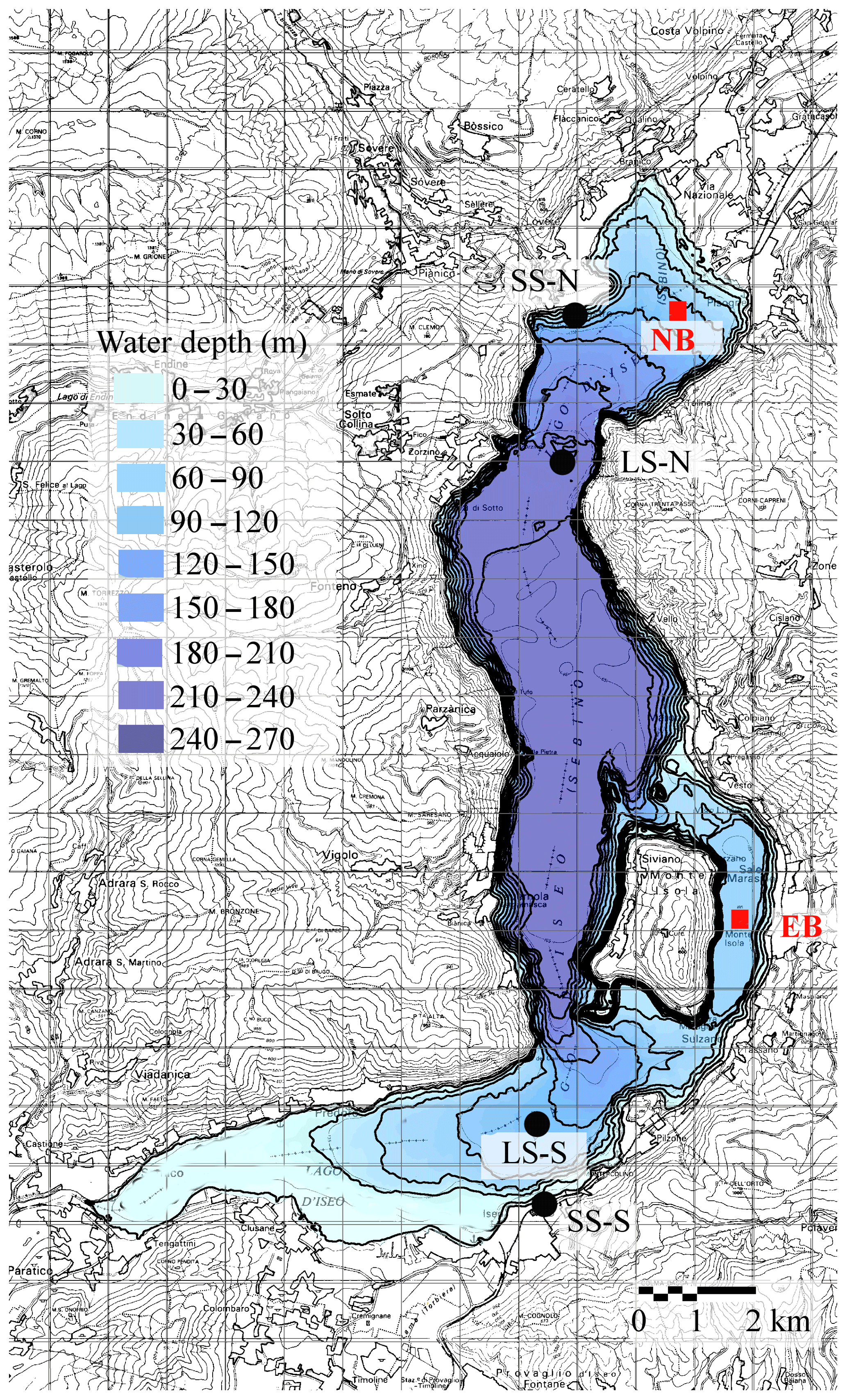
Figure 1 Contour of Lake Iseo bathymetry and isodepth lines at 30 m spacing. The black dots show the measurement stations located on the shore (SS) and in the lake (LS), both north and south. The red squares indicate the two points at 98 m in depth in the eastern basin (EB) and 105 m in the northern basin (NB) that are mentioned in the text.

2.2 Field data

A wide set of experimental data was measured at the lake stations shown in Fig. 1 to describe the wind-induced movements of the water layers in the mixolimnion and monimolimnion of Lake Iseo. Two onshore stations measured wind speed and direction, air temperature, air humidity, and shortwave radiation (SS-N and SS-S) at a high temporal resolution (60 s). Furthermore, a floating station (LS-N) measured wind speed and direction and net longwave radiation. LS-N is further equipped with 11 submerged loggers that measure the temperature (±0.01 ^∘C accuracy, 60 s interval), providing data regarding the vertical movements of the thermal profile (see Fig. 2b). During October 2017, we added three additional temperature loggers at 55, 75 and 113 m in depth to better describe the temperature fluctuations below the thermocline given their higher accuracy (±0.002 ^∘C).

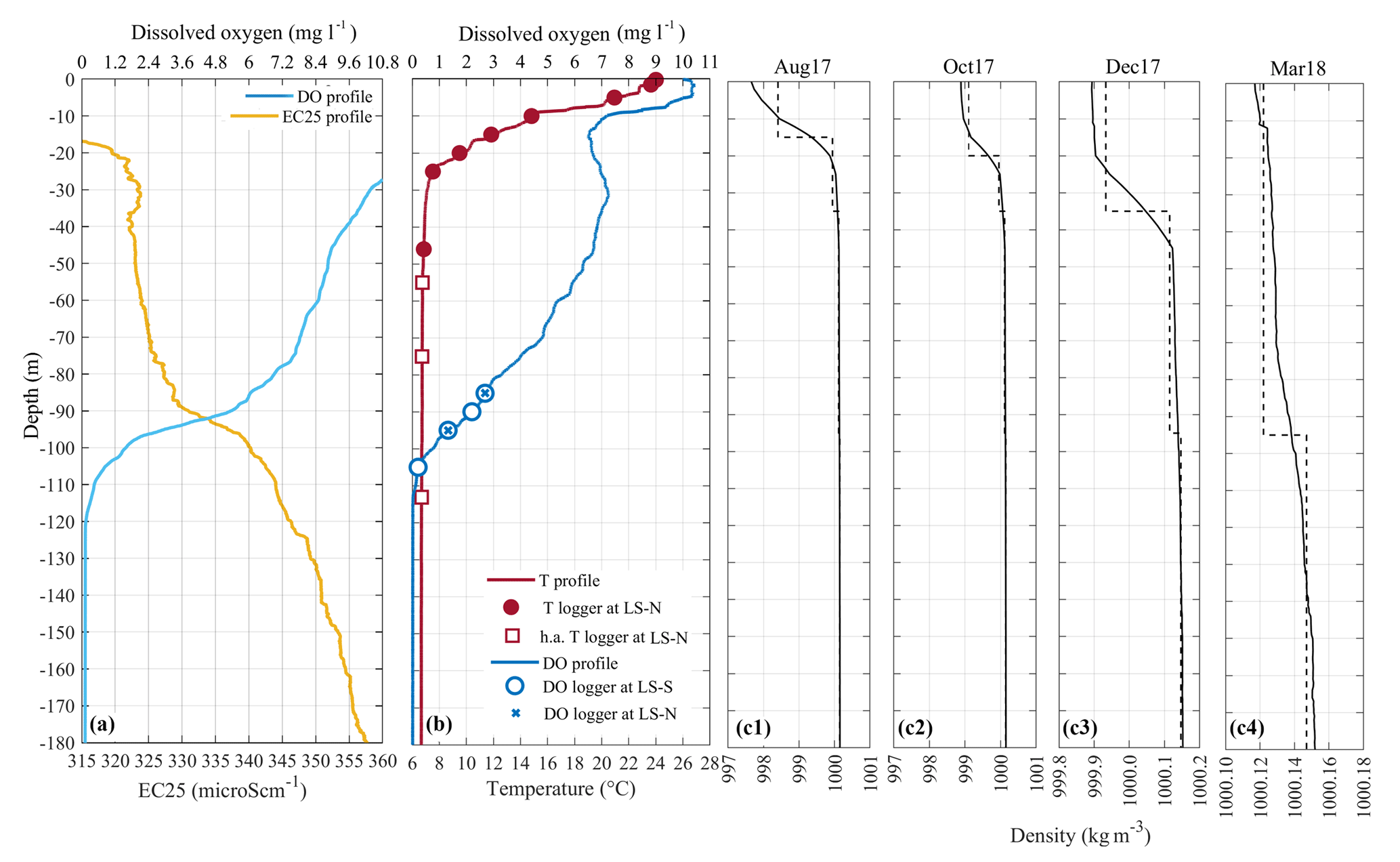
Figure 2 (a) Vertical profile of temperature-compensated conductivity (EC25) and dissolved oxygen (DO) measured on 10 April 2018 at LS-N. (b) Vertical profile of temperature (T) and dissolved oxygen (DO) measured on 22 July 2017 at the LS-N. The circles and the crosses show the DO sensors at LS-S and LS-N, respectively. The dots and the squares show the depth of the temperature sensors at LS-N, with the squares indicating the high-accuracy sensors. (c1–c4) Vertical profiles of monthly averaged density (solid lines) during 4 months and the corresponding discrete layered structure (dashed line) used in the modal model. The density profiles were calculated on the basis of an empirical equation of state that relates density to conductivity and temperature, calibrated for Lake Iseo according to the algorithm by Moreira et al. (2016) (details are in Scattolini, 2018).

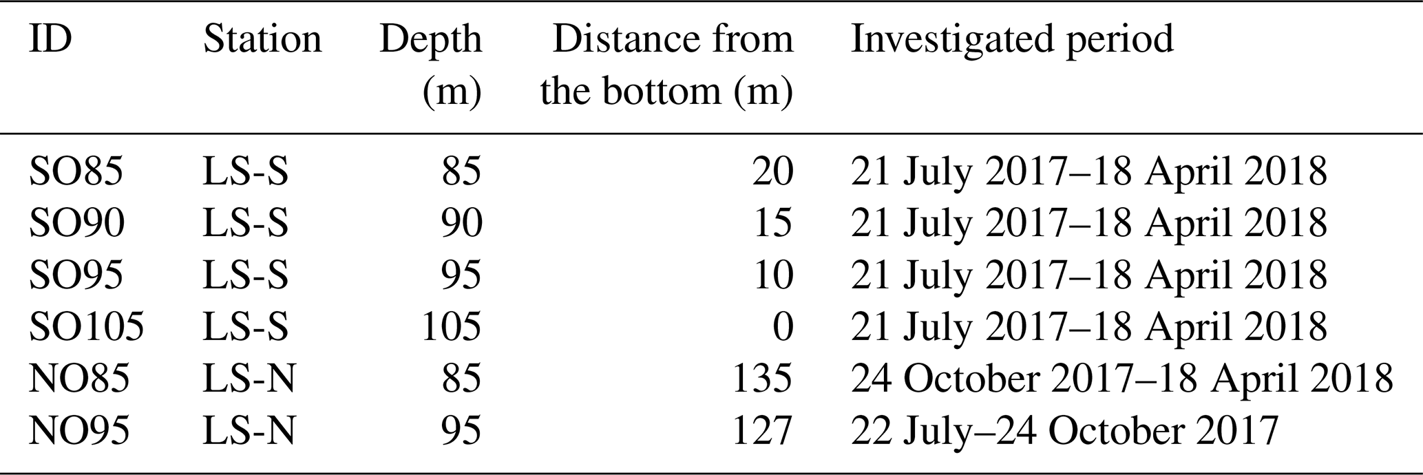
The LS-S logger chain was installed at 105 m in depth in the southern basin. To capture the vertical fluctuations in the oxycline, we installed four submersible instruments (miniDOT, Precision Measurement Engineering, Vista, Ca, USA) between 85 and 105 m in depth, and measured dissolved oxygen (DO) for 9 consecutive months at a 60 s⁻¹ sampling frequency (see Table 1). These loggers rely on a fluorescence-based oxygen measurement with an accuracy of ±5 % of the measured value (mg L⁻¹). Two miniDOT loggers were also installed at the northern station (LS-N) at 85 and 95 m in depth. As shown in Table 1, NO85 and NO95 measured the oxygen concentration at the same depths as those of the southern instruments but operated for a shorter period of time. In the following sections, we will focus on describing the data analysis from July 2017 to February 2018 that fully captures the oxygen concentration evolution during the transition from a strongly to a weakly stratified period.

Table 1 Overview of the oxygen measurements in Lake Iseo (sampling frequency of 60 s⁻¹).

On 21 and 22 July 2017, we also conducted a field campaign aimed at investigating the oxygen profiles in the whole water column at a higher vertical resolution. Using a conductivity, temperature and depth (CTD) probe (RINKO CTD profiler with an optical fast DO sensor, JFL Advantech Co. Ltd., Tokyo, Japan), we alternately measured the temperature and DO profiles at the two lake extremities in the proximity of the LS-N and LS-S stations several times throughout the day. During the 2-day field campaign we installed miniDOT logger at 90 m in depth at LS-N, sampling a DO data every 60 s. Similarly, consecutive DO profiles were measured in the proximity of the LS-N stations on 10, 16 and 18 April 2018.

2.3 Numerical models

In this study we used two numerical models to evaluate dynamic aspects of the measured internal oscillations. Therefore, we quantified the temporal evolution of the periodicity and the spatial structure of the free modes in Lake Iseo.

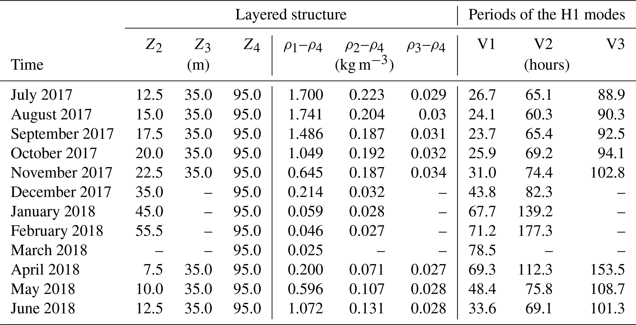
During the first stage, following the approach pursued in Guyennon et al. (2014) for Lake Como, a modal analysis was performed to quantify the temporal evolution of the free mode periods. This model subdivides a lake into constant density layers and provides the free baroclinic oscillations of the layer interfaces by solving an eigenvalue problem (details are in Guyennon et al., 2014). The Lake Iseo bathymetry was discretized using a 160 m  ×160 m horizontal grid, while the horizontally averaged vertical density profile was discretized monthly with the number of layers ranging from two to four, as detailed in Table 2. As is typical for the subalpine deep lakes, beginning in April, a pronounced three-layer thermal stratification develops, characterized by a well-mixed and warm surface layer, separated from the cold hypolimnion by an intermediate metalimnion. Under this condition, the upper interface of the metalimnion (Z₂ in Table 2) was set at the depth of the maximum temperature gradient (thermocline), while the lower interface (Z₃ in Table 2) was set at a depth of 35 m, below which the vertical temperature gradient strongly weakens. Typically, stronger thermal stratification occurs during August. After the thermocline deepening during the cooling period, the thermal stratification reduces to two layers during winter, separated by one interface between 35 and 55 m and characterized by a weak thermal gradient, which finally disappears during March. The thermal stratification of Lake Iseo is also superimposed by a chemical stratification. Accordingly, we considered an additional deep layer separated from the hypolimnion by the chemocline at 95 m in depth (Z₄ in Table 2), which is characterized by a 25 mg L⁻¹ step in density because of the higher concentration of dissolved salts. This value was quantified based on the chemical analysis of two water samples collected at 40 and 200 m in depth, according to the procedure proposed by Boehrer et al. (2010) (details are in Scattolini, 2018). The resulting discrete density structure describes the density profiles computed from the conductivity and temperature profiles well (see Fig. 2c).

Table 2 Features of the first horizontal and first, second and third vertical modes in Lake Iseo during a 1-year period. The monthly-averaged layered structure used for the calculation includes the depth Z_i of the upper interface of each ith layer and its density difference with respect to the deepest layer, ρ_i–ρ₄.

The vertical and horizontal structures of the free modes were investigated in detail by using a three-dimensional (3-D) hydrodynamic model that accounts for the nonlinear terms of the momentum equations. We used the hydrostatic version of the Hydrodynamic-Aquatic Ecosystem Model (AEM3D, Hodges and Dallimore, 2016). This model was developed from the ELCOM-CAEDYM model (Hodges et al., 2000) and has already been successfully tested in simulating the internal wave activity in the upper 50 m of Lake Iseo (Valerio et al., 2017). In particular, we investigated the wind-induced oscillations at approximately 100 m in depth, using a vertical grid of 150 layers and 1 m in thickness, followed by layers with gradually increasing thickness up to 25 m for the deepest part of the lake. We also refined the uniform horizontal grid up to 80 m ×80 m to better describe the bathymetry in the southern and northern areas. Finally, we used a passive tracer to follow the wind-driven vertical fluctuations in the oxycline. To simulate the structure of each single mode of oscillation, we conducted numerical experiments in which the lake was forced by a synthetic sinusoidal wind time series, with a maximum amplitude of 5 m s⁻¹, whose spatial and temporal structure fits that predicted by the eigenmodel for the free oscillation modes. This approach was already successfully applied by Vidal et al. (2007) to the study of the higher vertical modes of Lake Beznar.

3 Results

3.1 Analysis of the measured data

The oscillatory motions measured around the thermocline and the oxycline show marked differences in periodicities and amplitudes. These differences clearly stand out from the comparison of the 12 ^∘C isotherm oscillation at LS-N (see Fig. 3a) and the 0.5 mg DO L⁻¹ oscillation at LS-S (see Fig. 3c). To better analyze the frequency content of these time series we used the wavelet analysis. We applied the Morlet transform to the two measured signals that, unlike the classical Fourier transform, allows localization of the signals in both frequency and time rather than in the frequency space only (Torrence and Compo, 1998).

Figure 3 (a) Time series of the vertical displacements of the 12 ^∘C isotherm (white line) measured at LS-N, superimposed on the interpolated temperature distribution between 0 and 40 m, and (b) the associated continuous wavelet transform for the period between 23 July and 21 November 2017. (c) Time series of the vertical displacements of the 0.5 mg DO L⁻¹ isoline measured at LS-S, superimposed on the interpolated distribution of oxygen, and (d) the associated continuous wavelet transform. (e) Natural periods of the V1H1, V2H1 and V3H1 modes superimposed on the continuous wavelet transform of the N–S component of the wind measured at LS-N. The grey shaded regions on either end indicate the cone of influence, in which edge effects become important. The three rectangles with a black outline show the three periods analyzed in the following Figs. 4–6.

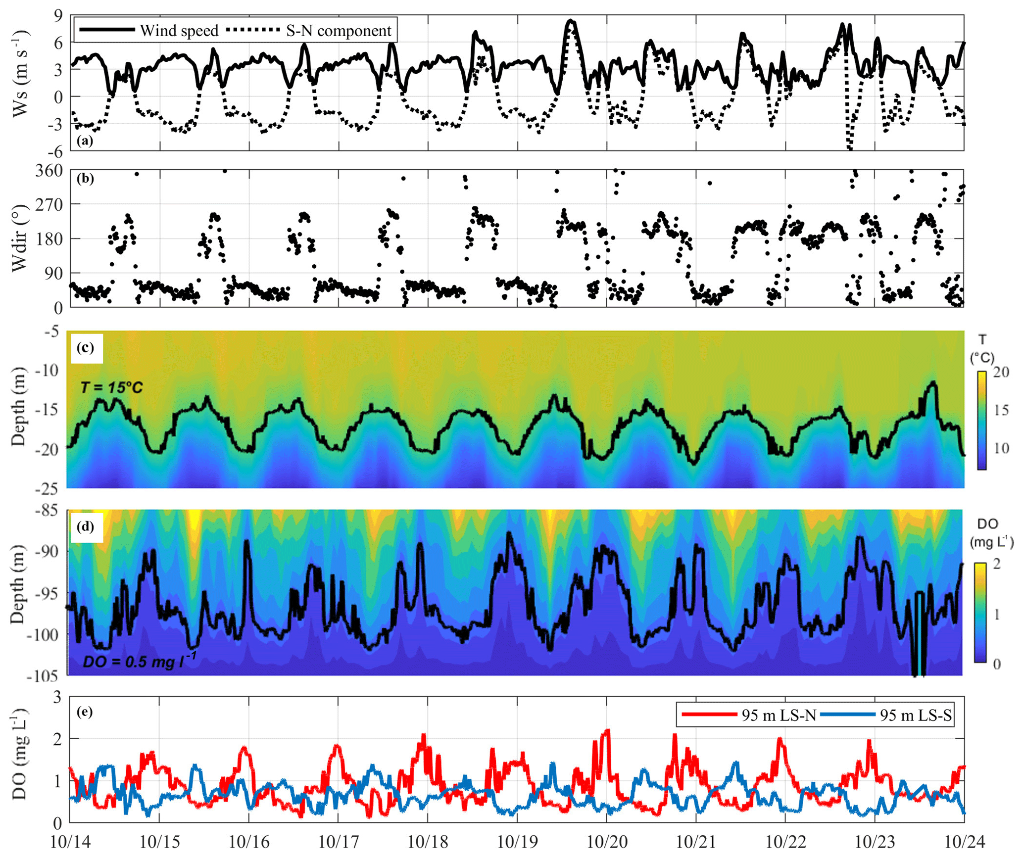
Figure 4 Time series measured from 14 to 24 October 2017 of (a) wind speed and its southerly component and (b) wind direction at LS-N, followed by the spatial and temporal variation in (c) temperature between 5 and 25 m in depth at LS-N and of (d) DO between 80 and 105 m at LS-S. Panel (e) compares the time series of DO measurements at the LS-N and LS-S stations. Corresponding to each tick of the horizontal axis is the time 00:00.

Figure 5 Same as Fig. 4 but referring to the period of 28 August–7 September 2017.

Figure 6 Same as Fig. 4 but referring to the period 5–18 December 2017.

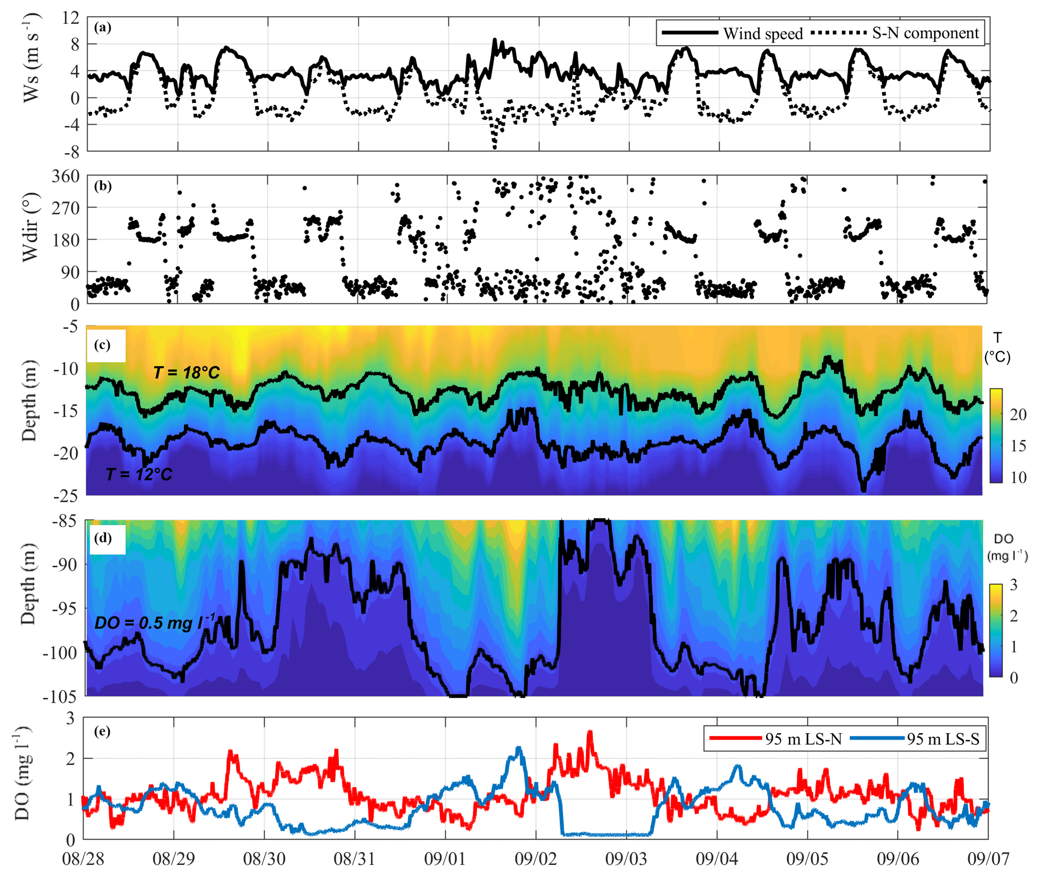
Figure 3b highlights the strong concentration of the energy of the shallower oscillations for an approximately 1-day period during the thermally stratified period. The cooling period is characterized by higher energy peaks, with maximum values during November. A trend towards a longer period is also detectable. Conversely, the deeper DO oscillations (Fig. 3d) show higher energy content with a period ranging from 1 to 4 days during the observational phase: the first 2 months (August–September) are characterized by a stronger thermal stratification and four major peaks are detectable in the 2–4-day band; during the following 2 months (October–November), during the autumn cooling, the energy level is lower and is centered at approximately 1 day; during the final 2 months (December–January), when the thermal stratification is weak, the energy peaks maximize and are sparse in the 2–4-day band.

To better highlight these different behaviors, we individually show an analysis of a representative fraction of each of these periods in Figs. 4 to 6. Figure 4 shows the third week of October when the oscillatory motions at the depth of the thermocline and of the oxycline have energy peaks centered around a daily period (see Fig. 3). During this week, the wind speed and direction show a typical pattern of the pre-alpine lakes (Valerio et al., 2017), blowing regularly from the south during the day and the north during the night. The internal wave response in the upper 30 m is a regular daily motion with an amplitude of approximately 6 m. Deeper in the water, the main vertical fluctuations at LS-S show a similar response in terms of both amplitude and periodicity, even though they are less regular and superimposed on higher-frequency signals. The 0.5 mg L⁻¹ iso-oxygen at 95 m in depth at LS-S is dominated by a 1-day period wave oscillation in counterphase with respect to the 15 ^∘C isotherm at the other end of the lake, suggesting a H1V1 behavior (see Fig. 4e). Consistently, the DO signals at 95 m in depth at LS-S and LS-N are in counterphase (see Fig. 4e).

On 21 and 22 July 2017, when a similar situation dominated by a V1H1 mode was present, we measured several temperature and oxygen vertical profiles around the thermocline and the oxycline at the LS-N and LS-S stations to better understand the vertical structure of this motion (see Fig. 7). One can easily see that the downwelling that characterizes the epilimnetic waters at LS-N is also present in the deeper layer of the oxycline, although it is vertically amplified and has a more irregular behavior. A similar structure characterizes the simultaneous upwelling at the LS-S station.

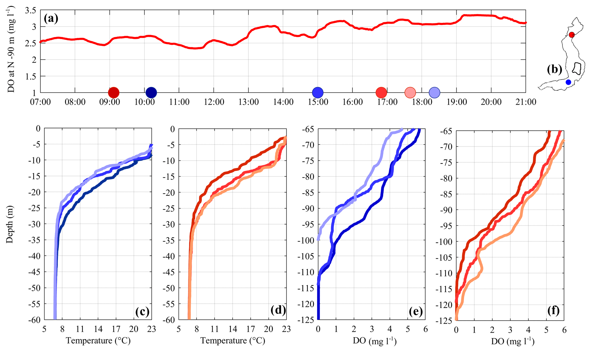
Figure 7 (a) DO concentration at 90 m in depth recorded at station LS-N on 21 July 2017. Colored dots on the x axis indicate the sampling time of the vertical profiles shown in (c–f). Panels (c) and (d) compare the profiles of temperature between 0 and 60 m, while panels (e) and (f) compare the profiles of DO between 65 and 125 m. Red and blue colors refer to the northern and southern sampling locations (see b), respectively.

A completely different oscillatory response developed during the period 28 August–7 September 2017, when the continuous wavelet transform highlights the different frequency content of the upper and deeper motions (Fig. 3). Consistently, in Fig. 5 the temperature and oxygen contours appear to be decoupled at the different depths. The upper 35 m (Fig. 5c) shows the superimposition of a dominant 1-day V1H1 oscillation and a lower-amplitude, longer-period (approximately 3 days), second vertical (V2) oscillation mode. The latter is qualitatively evident in Fig. 5c after a strong northerly wind started on 1 September, inducing a distinctive metalimnion widening on 2 September, followed by a metalimnion narrowing on 3 September. Low-pass filtering of the 12 ^∘C oscillations with an ∼1- and ∼3-day cutoff period resulted in average amplitudes of 3.3 and 2.2 m, respectively. Deeper in the water (see Fig. 5d), the internal wave field is instead dominated by much larger excursions of the oxycline (up to 20 m) and longer periodicities. Low-pass filtering of the 0.5 mg L⁻¹ iso-oxygen line at LS-S shows that the main oscillation pattern resembles the superimposition of an ∼3-day period oscillation with an average 14.6 m amplitude and a daily oscillation with an average 2.2 m amplitude. The observed lower-frequency motion presents a V2H1 structure, as shown in Fig. 5e in which the ∼3-day oscillation of the DO immediately above the oxycline is in counterphase at LS-N and LS-S. Figure 5c, d also show that the metalimnion widening at LS-N (e.g., on 2 September), associated with a downwelling in the hypolimnion, synchronously occurs with a hypolimnetic upwelling at LS-S. Accordingly, during the period under consideration, the field data suggest the dominance of a V1H1 mode in the epilimnion and a V2H1 mode in the hypolimnion.

From 16 to 18 April 2018, when a similar situation dominated by V2H1 was observed in the hypolimnion, we measured vertical profiles to examine the vertical structure of this motion at a higher spatial resolution. The DO time series measured at LS-N and LS-S at the oxycline depth (see Fig. 8a) shows a distinctive H1 oscillation with a period of approximately 4 days. In correspondence to the maximum and minimum vertical excursion of this fluctuation, we compared the vertical temperature and oxygen profiles at LS-N around the thermocline and the oxycline, respectively. In contrast to that shown in Fig. 7, the oscillation is not vertically uniform: a downwelling of the thermocline on the order of a few meters is associated with an upwelling of the oxycline of approximately 25 m. Accordingly, these data further highlight the amplification of the vertical excursion of the V2H1 motion in the oxycline area.

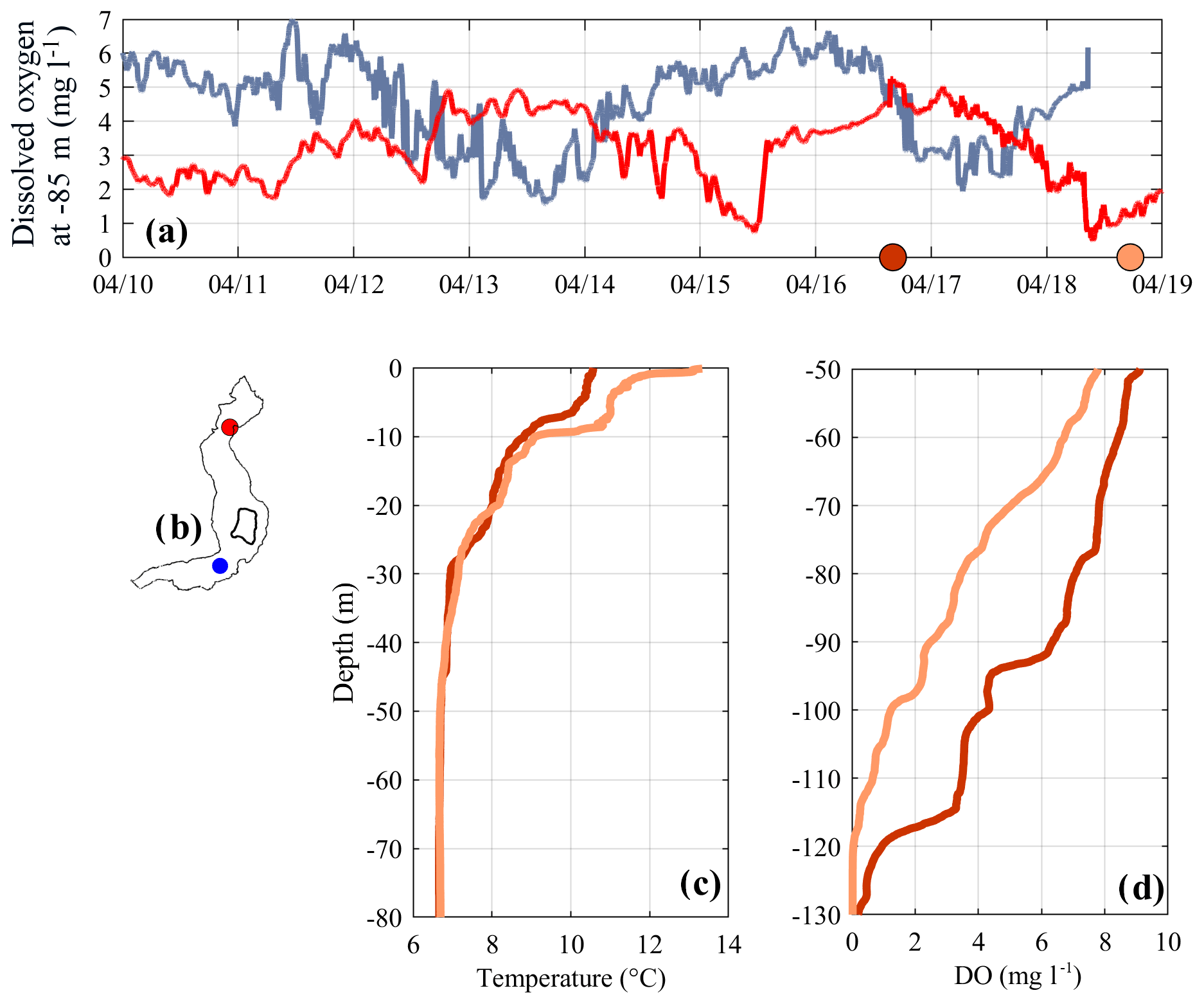
Figure 8 (a) Time series of DO measured at 85 m in depth on April 2018. Red and blue lines refer to the northern and southern sampling locations, respectively (see b). Colored dots on the x axis indicate the sampling time of the vertical profiles shown in (c–d). Panel (c) compares the profiles of temperature between 0 and 80 m in depth at LS-N, while panel (d) compares the profiles of DO between 50 and 130 m at LS-N.

In comparison to the previous oscillations, an intermediate case is shown in Fig. 6. In this case, during winter of 2017, the water column is weakly thermally stratified and the wind blows mostly from the north (see Fig. 6b). The wavelet transform of the DO measurements at LS-S show a first tight peak at an approximately 1∕4 day⁻¹ frequency and a second at an approximately 1∕2 day⁻¹ frequency (see Fig. 3d). Consistently, the time series of the 0.3 mg DO L⁻¹ measured at LS-S (see Fig. 6d) shows evidence of both a shorter and a longer period signal. Filtering with the cutoff periods highlighted in the spectrum shows that these ∼2- and ∼4-day signals have in this case comparable amplitudes (5.0 and 7.6 m, respectively) around the chemocline at LS-S. At LS-N, the DO time series at 85 m in depth oscillates in counter phase with respect to the southern series with coherent periodicities and amplitudes, thus suggesting an H1 response (see Fig. 6d).

3.2 Analysis of the model results

With reference to the modal results, Table 2 reports the monthly averaged values used for the calculations and the obtained yearly evolution of the periods of the V1H1, V2H1 and V3H1 modes. During April, all the periods present values (V1H1: 2.9, V2H1: 4.6 and V3H1: 6.4 days) that progressively decrease during the warming season. During the strongly stratified period (July–October) the modeled V1H1, V2H1 and V3H1 periods show nearly constant values, of approximately 1, 3 and 4 days, respectively. As soon as the water column starts cooling and the thermocline deepens, all mode periods start increasing. During the weaker three-layer stratification during February, when a similar density difference is present across the metalimnion and chemocline, V2H1 reaches a 7.4-day period, while the V1H1 period increases up to 3.3 days during March, when the water column is thermally homogeneous and only a saline stratification is present.

Regarding the spatial structure of these modes, Table S1 in the Supplement summarizes the 3-D results in terms of maximum interface displacements at different lake locations during four representative periods of the year. In the following, we mostly focus on the V1H1 and V2H1 oscillations of the thermocline (ξ₂) and the chemocline or oxycline (ξ₄) at LS-S and LS-N to provide an interpretation of the data measured at these stations from July 2017 to February 2018. Regarding the first vertical mode, all the interfaces oscillate in phase at the different depths. At LS-N (220 m depth), their amplitude is nearly vertically uniform (${\mathit{\xi }}_{\mathrm{4}}/{\mathit{\xi }}_{\mathrm{2}}\approx \mathrm{1}$), while at LS-S and NB (105 m depth) the intermediate and deep tilt is amplified (1.2<ξ₄∕ξ₂<2.3). Conversely, the deep interface tilt is strongly damped and more irregular in the eastern basin, a 100 m flat plateau located east of Monte Isola (${\mathit{\xi }}_{\mathrm{4}}/{\mathit{\xi }}_{\mathrm{2}}\approx \mathrm{0.4}$). In absolute terms, the weaker is the density stratification, the stronger is the interface tilt. At the end of winter, when the water column is thermally homogenous and chemically stratified, the V1H1 amplitudes are up to 7.5 times larger than those during summer. Regarding the second vertical mode, the interface oscillation is strongly nonuniform over the vertical direction, with the metalimnion and the chemocline both oscillating in counterphase with respect to the upper thermocline and with much larger vertical displacements. At LS-N, the vertical displacement of the chemocline is on average 2.6 times larger than that of the thermocline. This vertical amplification is favored by larger density gradients (at LS-N ξ₄∕ξ₂ decreases from 3.4 during August to 1.8 during December). Similarly to that observed for V1H1, this vertical amplification is also enhanced at the southern end of the lake (average ${\mathit{\xi }}_{\mathrm{4}}/{\mathit{\xi }}_{\mathrm{2}}=\mathrm{4.0}$ at LS-S), while it is strongly attenuated in the eastern basin, where the chemocline oscillations are more irregular in time and show maximum vertical displacements comparable to those of the thermocline (${\mathit{\xi }}_{\mathrm{3}}/{\mathit{\xi }}_{\mathrm{1}}\approx \mathrm{1}$). We emphasize that, independent from the vertical mode and stratification, the ratio between the V1H1 and V2H1 amplitude of a given interface simulated at different lake locations does not present a wide range of variation. In particular, the displacement of the deeper interface ξ₄ at the different locations is as follows: 0.6<ξ_4-LS-N∕ξ_4-LS-S<0.8; 0.1<ξ_4-EB∕ξ_4-LS-S<0.2; 0.7<ξ_4-NB∕ξ_4-LS-S<1.2. This implies that the chemocline maintains a similar H1 horizontal structure throughout the year, even with different absolute values depending on the stratification and the vertical mode (see Fig. S1 in the Supplement).

The obtained numerical results clarify the nature of the observed oscillations and extend the spatial information provided by the local measurements. Between October and November (see Fig. 4), we observed a daily coupled oscillatory response at the chemocline and thermocline. During this time, the natural period of V1H1 is daily as well, confirming that the whole water column is dominated by this type of motion. This is consistent with the observed spatial structure characterized by a counter-phase response at the two lake ends (H1) and a similar amplitude at the different depths (V1). During the strongly stratified period (August–September), we occasionally observed a decoupled internal wave response at the different depths (see Fig. 5). By comparing the periodicity of the measured oscillations and that of the unforced modes (see Fig. 3), the thermocline appears to be dominated by a V1H1 motion (∼1-day period), while the oxycline is dominated by a V2H1 motion (∼2–3-day period). This suggests that both modes were excited by the wind, but at different energy levels along the water column. This decoupled response can be explained by the vertical structure of the modes detailed in Table S1. During the summer stratification, the V1H1 amplitudes are nearly vertically uniform (1.1<ξ₄∕ξ₂<2.3). Conversely, the V2H1 amplitude at the chemocline ξ₄ is up to 5.7 times larger than that of the thermocline ξ₂. Accordingly, when a second vertical mode is excited by the wind, the larger vertical displacements occur at the deeper interface. This vertical amplification may explain why the V2H1 mode is dominant in the deeper waters and is in contrast weaker than the V1H1 daily signal around the thermocline. Finally, during the period from December to January (see Fig. 6) we observed the superimposition of ∼2- and ∼4-day large oscillations at the oxycline depth. According to the periodicities of the unforced modes, they correspond to V1H1 and V2H1 modes (see Fig. 3e). The evidence of a large-amplitude V1H1 mode at this depth is consistent with the increased displacements reported in Table S1 corresponding with the weaker density stratification.

Valerio et al. (2012) showed that the internal wave modes in the upper water layers are excited whenever the spatial and temporal structure of a wind field over a lake matches the surface velocity field of a particular internal mode. Accordingly, as shown in Fig. 3e, we superimposed the natural frequencies of the two main vertical modes with the continuous wavelet transform of the northerly components of the wind forcing to assess whether a fit in their periodicities might explain the observed internal wave motions. During the stratified period (July–November), most of the wind energy oscillates at a period of approximately 1 day, likely because of the regular alternation of northerly and southerly thermal winds, typical of the area (see Valerio et al., 2017). This forcing perfectly fits the V1H1 mode that is regularly excited and dominates the response of the upper waters (see Fig. 3b). Occasionally, the daily wind energy reduces its intensity when the wind blows longer from the same direction. From July to October 2017, this occurred three times (see Fig. 3e). Interestingly, corresponding to each of these events, there is a large energy peak in the oxycline oscillations for the lower frequencies (see Fig. 3d). The reason is a resonance between the wind and the waves: the longer periodicity of the wind forcing approaches the natural periodicity of the V2H1 mode, such that it is excited in place of V1H1, inducing large vertical fluctuations below the metalimnion. During the weakly stratified period, the thermal conditions in the surrounding watershed limit the intensity and the regularity of the alternating thermal winds, causing a spread of wind energy over a larger band of frequencies (see Fig. 3e). In contrast to that which occurred prior, this condition favors the excitation of a longer-period V1H1 oscillation that clearly is also evident at the oxycline depth, with amplitudes favored by the weak stratification.

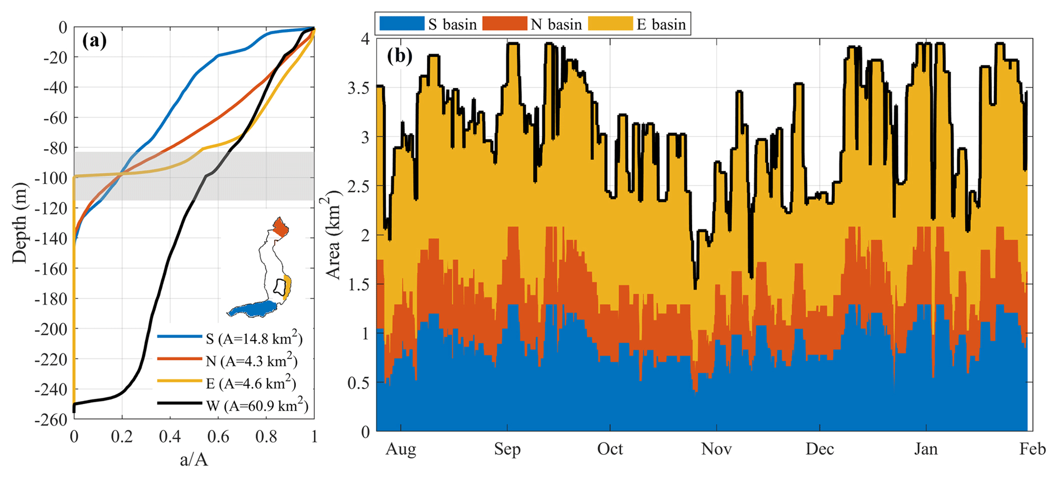
Figure 9 (b) Estimation of the area of the bottom sediments subjected to alternating redox conditions. The areas were calculated by considering the oscillations of the oxycline over a 3-day-long time window. The three colors make reference to the contribution of the southern (S, blue), northern (N, red) and eastern basins (E, yellow), as shown on the map. In (a), the area–depth curves indicate the cumulative area “a” of the bottom situated below a given water depth in the whole lake (W) and in each sub-basin (E, N, S). On the x axis, the area “a” was normalized with the total area “A” of each basin. The grey shaded area marks the maximum and minimum vertical displacement of the 0.5 mg DO L⁻¹ recorded at LS-S, highlighting the area of the bottom where the oxycline fluctuates.

4 Discussion and conclusions

In Lake Iseo reduced deep mixing has resulted in the formation of an anoxic monimolimnion below 95 m in depth, such that any vertical displacement of the oxycline may induce variation in redox conditions of the contiguous sediments. Accordingly, it seems reasonable to advance the hypothesis that the internal wave motions in Lake Iseo might result in unstable, unsteady sediment–water fluxes.

The data collected from July 2017 to February 2018 clearly support our initial hypothesis that there are large and periodic displacements of the oxycline. The typical oxycline oscillation in the southern basin is in the range of 10–20 m, with periods ranging from 1 to 4 days. Comparing these movements to those already studied in the lake's upper water layers (Valerio et al., 2012), dominated to a large extent by a 1-day motion, we found the dynamics in the deeper waters to be more irregular in character, featuring larger amplitudes at lower frequencies. We primarily attributed this behavior to the excitation of a V2H1 mode characterized by amplified vertical displacements below the thermocline. During weakly stratified conditions this behavior was explained by the excitation of a V1H1 mode, featuring lower frequencies and larger tilts because of the weaker density gradients. In both cases, the overlap of the temporal structure of the wind forcing with that of the two modes provides evidence for a resonant response to wind as observed, inter alia, by Vidal et al. (2007).

A primary role for the excitation of these deep internal wave motions is played by the permanent chemical stratification. In Lake Iseo, the decomposition of organic matter and the dissolution of its end products have favored the solute accumulation in the deeper waters since the 1980s. Accordingly, a stable density gradient is present between the oxic mixolimnion and the anoxic monimolimnion, contributing to maintaining the latter isolated from the water above. This condition allows for the occurrence of large baroclinic motions at the interface of these layers, even if the water column is thermally homogenous. Accordingly, this work provides experimental and numerical evidence of a chemical gradient supporting deep baroclinic motions in perennially stratified lakes, as already numerically argued by Salvadé et al. (1988) in Lake Lugano, where a similar density stratification occurs.

The observations of highly energetic V2H1 motions in Lake Iseo broaden the observations of higher vertical modes, which have been much less frequently reported in lakes with respect to the first vertical mode (e.g., Wiegand and Chamberlain, 1987; Münnich et al., 1992; Roget et al., 1997) and rarely reported in deep lakes (e.g., Boehrer 2000; Boehrer et al., 2000; Appt et al., 2004; Guyennon et al., 2014). Interestingly, stronger evidence of these motions in the deep waters compared to the upper waters supports the idea by Hutter et al. (2011) that the reason for rare documentation in the literature of these motions is not because they are not excited but that the measuring techniques usually are not sufficiently detailed to capture them. Moreover, if typically their excitation is seen to be favored by the presence of a thick metalimnion, in this case they are enhanced by the presence of a chemical stratification in the deeper waters. Conducting a sensitivity analysis on the density stratification used as the initial condition for the simulations, we observed, for example, that during August the amplitude of the second vertical modes is from 2 to 3 times greater compared to a case in which the chemical stratification is absent. Interestingly, similar observations of higher baroclinicity supported by deep isopycnal layers have been observed in other environments corresponding to vertical salinity gradients (South Aral Sea by Roget et al., 2017) and turbidity (Ebro Delta by Bastida et al., 2012).

The observation of a pronounced spatiotemporal oxycline dynamics supports the hypothesis of the occurrence of alternating redox conditions in the water above the sediments at the bottom of Lake Iseo. For example, considering the variations in DO concentration at 95 m of depth in panel (d) of Figs. 4 to 6, one can observe that the sediment surface at this depth is periodically forced by a variation in DO concentrations in the overlying water between 0 and 3 mg L⁻¹. To quantify the potential biogeochemical implications of the oxycline dynamics in Lake Iseo, it is important to estimate the areal extent of sediment subjected to alternating redox conditions. Obviously, the smaller the bed slope, the larger the sediment area impacted by a given vertical oxycline displacement. Accordingly, areas subjected to alternating redox conditions will mainly be located in the northern, southern and eastern sub-basins (see Fig. 9a), where the bottom more gradually rises compared to that of the central basin. The depth–area relationship of the three sub-basins (see Fig. 9a) shows that approximately 5 km² of sediment area is situated between the depths of 85 and 115 m, representing the upper limit of the area subjected to episodic changes in oxygen availability. However, a more precise calculation requires knowledge of the spatial pattern of the oxycline oscillations in the three sub-basins. To this end, we coupled the area–depth curve of the southern basin to the time series of vertical displacements of the 0.5 mg DO L⁻¹ iso-oxygen line at LS-S, taken as a reference for the oxycline depth. The same analysis was also extended to the northern and eastern basins, where we used the spatial distribution of the deeper layer interface provided by the 3-D numerical model to estimate the oxycline oscillations (see Table S1). The resulting basin-specific areas subjected to alternating redox conditions (typically with variations higher than 1 mg L⁻¹) are shown in Fig. 9b.

We estimated that, overall, 1.9 km² of bottom sediments of Lake Iseo, 3 % of the whole area, is on average subjected to alternating redox conditions with periods of from 1 to 4 days, with a maximum areal extent during summer, when long-lasting winds favor the excitation of a second vertical mode, and from January to February, when the weak thermal gradients favor strong tilts in the chemocline. The relative contributions of the sub-basins to the whole area subjected to alternating redox conditions are 49 % (southern basin), 32 % (northern basin) and 19 % (eastern basin). Because of its conformation as a horizontal plateau with a typical depth of 100 m, the eastern basin contributes only if the oxycline is above 100 m in depth.

Oxycline dynamics affect lake sediments with implications for the redox-controlled biogeochemical processes therein. Redox-sensitive P release (Søndergaard, 2003) may be halted in sediment depth segments affected by oxycline oscillations and shift P towards redox-insensitive fractions (Parsons et al., 2017). However, the role of sediments as sinks and sources of P is known to be controlled by a suite of diagenetic processes including P supply, microbial mineralization, and interaction between iron and sulfur (Hupfer and Lewandowski, 2008). The susceptibility of these processes to excursion in oxygen availability is less well understood. According to our calculations, an additional 3 % of the sediment area is affected by such excursions. The monimolimnion of Lake Iseo stores the vast majority of the in-lake P (360 t of 480 t, April 2016, Michael Hupfer, personal communication, 2018), indicating the relevance of P release from sediment below the oxycline. Therefore, it remains crucial to further explore the dynamics in redox forcing in sediments of perennially stratified lakes and the entailing implications for internal P cycling and biogeochemical turnover.