the Creative Commons Attribution 4.0 License.
the Creative Commons Attribution 4.0 License.
 | 25 Feb 2019
Technical note: Analytical sensitivity analysis and uncertainty estimation of baseflow index calculated by a two-component hydrograph separation method with conductivity as a tracer
Weifei Yang
Changlai Xiao
Xiujuan Liang
The two-component hydrograph separation method with conductivity as a tracer is favored by hydrologists owing to its low cost and easy application. This study analyzes the sensitivity of the baseflow index (BFI, long-term ratio of baseflow to streamflow) calculated using this method to errors or uncertainties in two parameters (BFC, the conductivity of baseflow, and ROC, the conductivity of surface runoff) and two variables (yk, streamflow, and SCk, specific conductance of streamflow, where k is the time step) and then estimates the uncertainty in BFI. The analysis shows that for time series longer than 365 days, random measurement errors in yk or SCk will cancel each other out, and their influence on BFI can be neglected. An uncertainty estimation method of BFI is derived on the basis of the sensitivity analysis. Representative sensitivity indices (the ratio of the relative error in BFI to that of BFC or ROC) and BFI′ uncertainties are determined by applying the resulting equations to 24 watersheds in the US. These dimensionless sensitivity indices can well express the propagation of errors or uncertainties in BFC or ROC into BFI. The results indicate that BFI is more sensitive to BFC, and the conductivity two-component hydrograph separation method may be more suitable for the long time series in a small watershed. When the mutual offset of the measurement errors in conductivity and streamflow is considered, the uncertainty in BFI is reduced by half.
- Article
(588 KB) - Full-text XML
-
Supplement
(601 KB) - BibTeX
- EndNote


Hydrograph separation (also called baseflow separation), aims to identify the proportion of water in different runoff pathways in the export flow of a basin, which helps in identifying the conversion relationship between groundwater and surface water; in addition, it is a necessary condition for optimal allocation of water resources (Cartwright et al., 2014; Miller et al., 2014; Costelloe et al., 2015). Some researchers indicated that tracer-based hydrograph separation methods yield the most realistic results because they are the most physically based methods (Miller et al., 2014; Mei and Anagnostou, 2015; Zhang et al., 2017). Many hydrologists have suggested that electrical conductivity can be used as a tracer in hydrograph separation (Stewart et al., 2007; Munyaneza et al., 2012; Cartwright et al., 2014; Lott and Stewart, 2016; Okello et al., 2018). Conductivity is a suitable tracer because its measurement is simple and inexpensive, and it has distinct applicability in long-series hydrograph separation (Okello et al., 2018).
The two-component hydrograph separation method with conductivity as a tracer (also called conductivity mass balance (CMB) method; Stewart et al., 2007) calculates baseflow through a two-component mass balance equation. The general equation is shown in Eq. (1), which is based on the following assumptions:
- a.
contributions from end-members other than baseflow and surface runoff are negligible;
- b.
the specific conductance of runoff and baseflow are constant (or vary in a known manner) over the period of record;
- c.
in-stream processes (such as evaporation) do not change specific conductance markedly;
- d.
baseflow and surface runoff have significantly different specific conductance.
where b is baseflow (L3 T−1), y is streamflow (L3 T−1), SC is the electrical conductivity of streamflow, and k is time step number. The two parameters BFC and ROC represent the electrical conductivity of baseflow and surface runoff, respectively.
Stewart et al. (2007) conducted a field test in a drainage basin of 12 km2 in southeast Hillsborough County, Florida, and showed that the maximum conductivity of streamflow can be used to replace BFC and the minimum conductivity can be used to replace ROC. However, Miller et al. (2014) pointed out that the maximum conductivity of streamflow may exceed the real BFC; therefore, they suggested that the 99th percentile of the conductivity of each year should be used as BFC to avoid the impact of high BFC estimates on the separation results and assumed that baseflow conductivity varies linearly between years. The determination of the parameters (BFC, ROC) of the conductivity two-component hydrograph separation method involves some uncertainties (Miller et al., 2014; Okello et al., 2018). Therefore, sensitivity analysis of parameters and quantitative analysis of the uncertainties will contribute towards further optimization of the CMB method and improving the accuracy of hydrograph separation.
Most existing parameter sensitivity analysis methods are empirical methods that usually substitute varying values of a certain parameter into the separation model and then compare the range of the separation results produced by these varying parameter values (Eckhardt, 2005; Miller et al., 2014; Okello et al., 2018). Eckhardt (2012) indicated that “An empirical sensitivity analysis is only a makeshift if an analytical sensitivity analysis, that is an analytical calculation of the error propagation through the model, is not feasible”. Eckhardt (2012) derived sensitivity indices of equation parameters by the partial derivative of a two-parameter recursive digital baseflow separation filter equation. Until now, the parameters' sensitivity indices of the CMB equation have not been derived.
At present, the uncertainty in the separation results of the CMB method is mainly estimated using an uncertainty transfer equation based on the uncertainty in BFC, ROC, and SCk (Genereux, 1998; Miller et al., 2014). See Sect. 3.1 for details. In this uncertainty estimation method, the uncertainty in the baseflow ratio (fbf, the ratio of baseflow to streamflow in a single calculation process) is estimated, and the average uncertainty in multiple calculation processes is then used to estimate the uncertainty in the baseflow index (BFI, long-term ratio of baseflow to total streamflow). This method can neither directly estimate the uncertainty in BFI nor consider the randomness and mutual offset of conductivity measurement errors, and, thus, it does not provide accurate estimates of BFI uncertainty.
The main objectives of this study are as follows: (i) analyze the sensitivity of long-term series of baseflow separation results (BFI) to parameters and variables of the CMB equation (Sect. 2); (ii) derive the uncertainty in BFI (Sect. 3). The derived solutions were applied to 24 basins in the US, and the parameter sensitivity indices and BFI uncertainty characteristics were analyzed (Sect. 4).
2.1 Parameters BFC and ROC
In order to calculate the sensitivity indices of the parameters, the partial derivatives of bk in Eq. (1) with respect to BFC and ROC are required (the derivation process is expressed as Eqs. A1 and A2):
For the convenience of comparison, the baseflow index (BFI) is selected as the baseflow separation result for long time series to analyze the influence of parameter uncertainty on BFI,
where b and y denote the total baseflow and total streamflow, respectively, over the whole available streamflow sequences, and n is the number of available streamflow data.
Then, the partial derivatives of BFI to BFC and ROC should be calculated (the derivation process is presented in Eqs. A3 and A4):
The definition of the partial derivative suggests that the influence of the errors in the parameters (ΔBFC and ΔROC) in Eq. (1) on the BFI can be expressed by the product of the errors and its partial derivatives. Then the errors in BFI caused by small errors in BFC and ROC can be approximated by
The dimensionless sensitivity indices (S) can be obtained by comparing the relative error in BFI caused by the small errors in BFC and ROC with that of BFC and ROC (see Eqs. B1 and B2):
where S(BFI|BFc) represent the dimensionless sensitivity index of BFI (output) with BFc (uncertain input) and S(BFI|ROc) with ROc.
The dimensionless sensitivity index is also called the “elasticity index”, and it reflects the proportional relationship between the relative error in BFI and the relative error in parameters (e.g., if S(BFI|BFc)=1.5 and the relative error in BFc is 5 %, then the relative error in BFI is 1.5 times 5 % = 7.5 %). After determining the values of BFC, ROC, BFI, y, yk, and SCk, the sensitivity indices S(BFI|BFc) and S(BFI|ROc) can be calculated and compared.
2.2 Variables yk and SCk
In addition to the two parameters, there are two variables (SCk and yk) in Eq. (1). This section describes the sensitivity analysis of BFI to these two variables. Similar to Sect. 2.1, the partial derivatives of bk in Eq. (1) to SCk and yk are obtained (see Eqs. A5 and A6), and the partial derivatives of BFI to SCk and yk are further obtained (see Eqs. A7 and A8):
According to previous studies (Munyaneza et al., 2012; Cartwright et al., 2014; Miller et al., 2014; Okello et al., 2018) and this study (Table 1), the difference between BFC and ROC is often greater than 100 µs cm−1. Therefore, is usually less than 0.01 cm µs−1. Appendix C shows that the value of is usually far less than 1 day m−3.
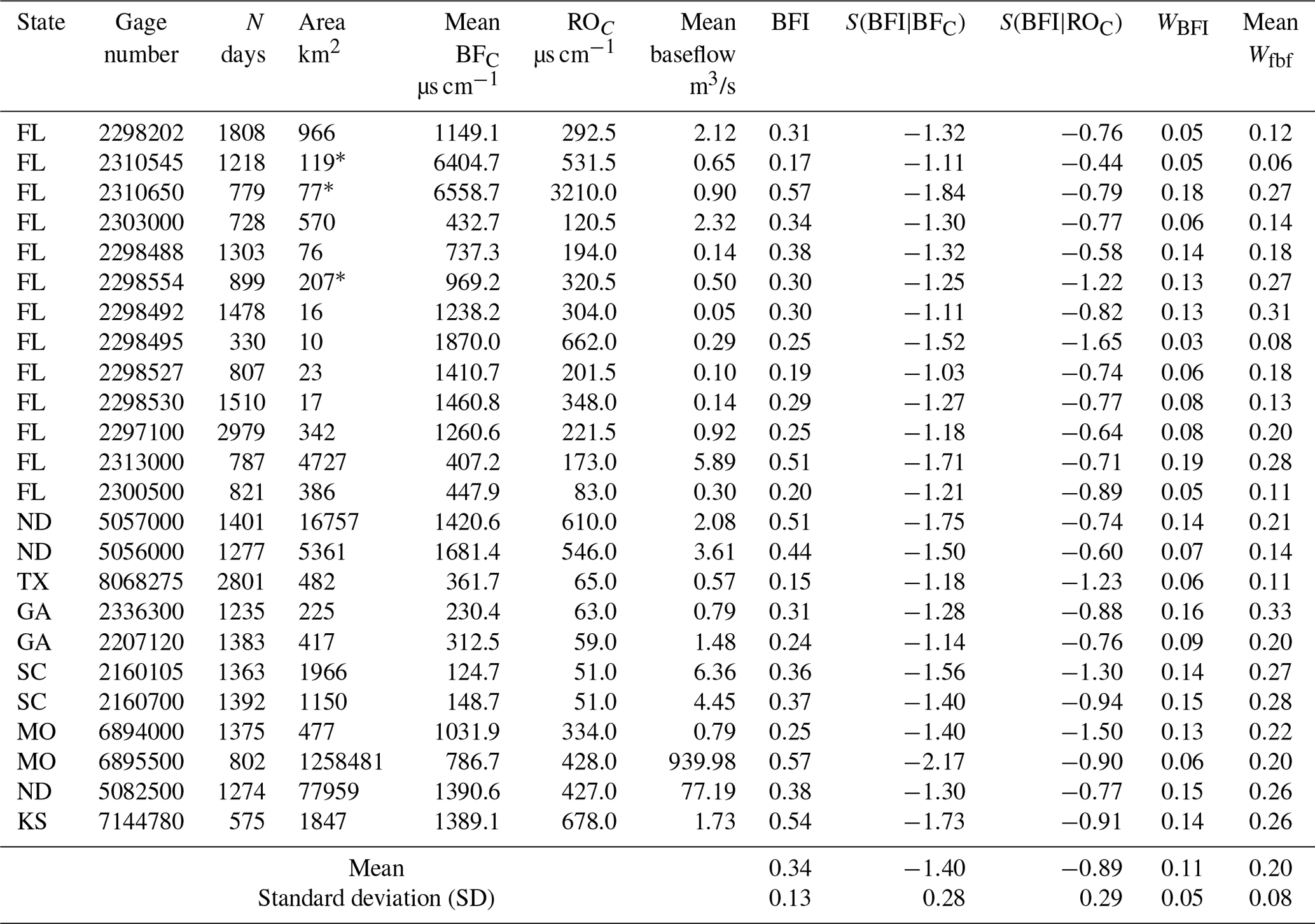
Table 1Basic information, parameter sensitivity analysis, and uncertainty estimation results for 24 basins in the US. The asterisk in the “area” column indicates that the values are estimated based on data from adjacent sites.
Small errors in SCk and yk cause errors in BFI:
The errors in BFI caused by SCk and yk are summed up to obtain the error in BFI caused by and in the whole time series:
Wagner et al. (2006) reported that the uncertainty in instruments is usually less than 5 % for SCk (<100 µs cm−1) and less than 3 % for SCk (>100 µs cm−1). According to Hamilton and Moore (2012), streamflow data from the US Geological Survey's (USGS) are often assumed by analysts to be accurate and precise within ±5 % at the 95 % confidence interval. In this study, the error ranges of SCk and yk are all considered to be ±5 %. The errors in SCk and yk mainly comprise random measurement errors which mostly follow a normal distribution or a uniform distribution (Huang and Chen, 2011). Considering the mutual offset of random errors, when the time series (n) is sufficiently long, in Eq. (15) and in Eq. (16) will approach zero.
The analysis of and under different time series (n) and different error distributions (normal distribution or uniform distribution) of a surface water station (USGS site number 0297100) showed that the random errors in daily average conductivity and streamflow have a negligible effect on BFI when the time series is greater than 365 days (see Supplement S1 for detail).
3.1 Previous attempts
According to previous studies, in the case where a variable g is calculated as a function of several factor x1, x2, x3, …, xn (e.g., g=G(x1, x2, x3, …, xn)) and based on the assumptions that the factors are uncorrelated and have a Gaussian distribution, the transfer equation (also known as Gaussian error propagation) between the uncertainty in the independent factors and the uncertainty in g is
where Wg, , , and are the same type of uncertainty values (e.g., all average errors or all standard deviations) for g, x1, x2, and xn, respectively. A more detailed description of this equation can be found in Taylor (1982), Kline (1985), and Ernest (2005).
According to Genereux (1998), “While any set of consistent uncertainty (W) values may be propagated using Gaussian error propagation, using standard deviations multiplied by t values from the Student's t distribution (each t for the same confidence level, such as 95 %) has the advantage of providing a clear meaning (tied to a confidence interval) for the computed uncertainty would correspond to, for example, 95 % confidence limits on BFI”.
Based on the above principle, Genereux (1998) substituted Eq. (18) into Eq. (17) to derive the uncertainty estimation equation (Eq. 19) of the CMB method:
where fbf is the ratio of baseflow to streamflow in a single calculation process, Wfbf is the uncertainty in fbf at the 95 % confidence interval, WBFC and WROC are the standard deviations of the BFC and ROC multiplied by the t value (α=0.05; two-tail) from the Student's distribution, and WSC is the analytical error in conductivity multiplied by the t value (α=0.05; two-tail) (Miller et al., 2014).
Better estimates of the uncertainty in fbf within a single calculation step can be obtained using Eq. (19). Hydrologists usually approximate the uncertainty in BFI by averaging the uncertainty in all steps (Genereux, 1998; Miller et al., 2014). However, this method does not consider the mutual offset of the conductivity measurement errors and cannot accurately reflect the uncertainty in BFI. In this study, an uncertainty estimation equation of BFI is derived on the basis of the parameter sensitivity analysis.
3.2 Uncertainty estimation of BFI
BFI is a function of BFc, ROc, SCk, and yk. In addition, the uncertainties in BFc, ROc, SCk, and yk are independent of each other. As explained earlier (Sect. 2.2), the random errors in daily average conductivity and streamflow have a negligible effect on BFI when the time series (n) is greater than 365 days (1 year); therefore, the uncertainty in BFI can be expressed as
Then, Eq. (20) can be rewritten as
where WBFI, WBFC, and WROC are the same type of uncertainty values for BFI, BFC, and ROC, respectively, as described above.
4.1 Data and processing
The above sensitivity analysis and uncertainty estimation methods were applied to 24 catchments in the US (Table 1). All basins used in this study are perennial streams, with drainage areas ranging from 10 to 1 258 481 km2. Each gage has about at least 1 year of continuous streamflow and conductivity for the same period of records. All streamflow and conductivity data are daily average values retrieved from the USGS National Water Information System (NWIS) website: http://waterdata.usgs.gov/nwis (last access: September 2018).
The daily baseflow of each basin was calculated using Eq. (1). The 99th percentile of the conductivity of each year was used as BFC, and linear variation in baseflow conductivity between years was assumed. The first percentile of the conductivity of the whole series of streamflow in each basin was used as the ROC. The total baseflow b, total streamflow y, and baseflow index BFI of each watershed were then calculated. According to the results of the hydrograph separation, the parameter sensitivity indices of BFI for mean BFC (S(BFI|BFc)) and ROC (S(BFI|ROc)) were calculated using Eqs. (9) and (10), respectively.
Finally, the uncertainty in fbf in each step was calculated using Eq. (19) and averaged to obtain the mean Wfbf for each basin. The uncertainty (WBFI) in BFI was directly calculated using Eq. (23), and then the values of mean Wfbf and WBFI were compared. For each basin, WBFC is the standard deviation of the BFC of the whole series multiplied by the t value (α=0.05; two-tail) from the Student's distribution, WROC is the standard deviation of the lowest 1 % of measured conductivity multiplied by the t value (α=0.05; two-tail) from the Student's distribution, and WSC is the analytical error in the conductivity (5 %) multiplied by the t value (α=0.05; two-tail).
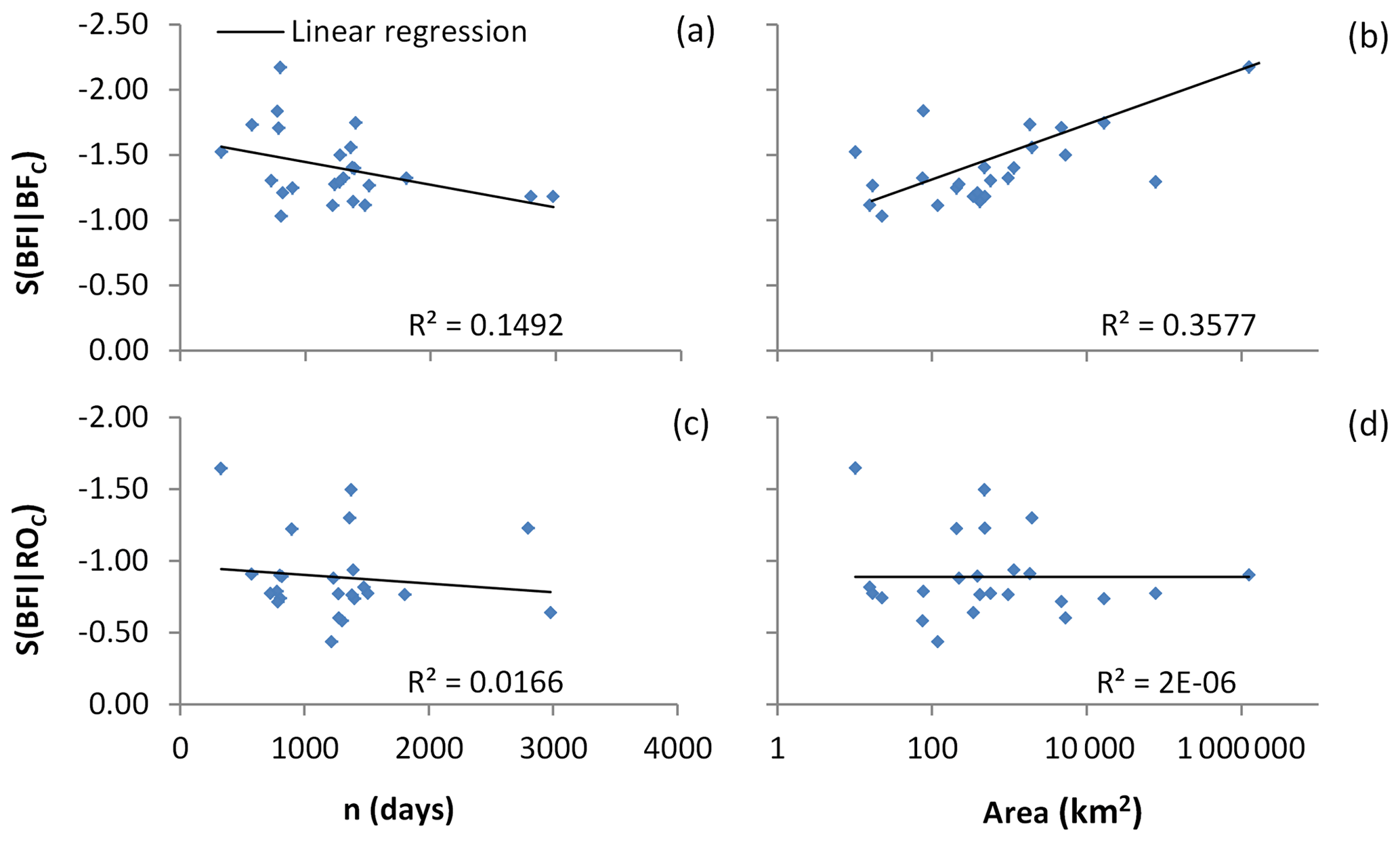
Figure 1Scatterplots of sensitivity indices vs. time series (n) and drainage area of the 24 US basins. The watershed area uses a logarithmic axis, while the others are linear axes.
4.2 Results and discussion
The calculation results are shown in Table 1. The average baseflow index of the 24 watersheds is 0.34, the average sensitivity index of BFI for mean BFC (S(BFI|BFc)) is −1.40, and the average sensitivity index of BFI for ROC (S(BFI|ROc)) is −0.89. The negative sensitivity indices indicate negative correlations between BFI and BFC (ROC). The absolute value of the sensitivity index for BFC is generally greater than that for ROC, indicating that BFI is more affected by BFC – for example, if there are 10 % uncertainties in both BFC and ROC, then BFC leads to −1.40 times 10 % of uncertainty in BFI (−14.0 %), while ROC leads to −0.89 times 10 % (−8.9 %). Therefore, the determination of BFC requires more caution, and any small error may lead to greater uncertainty in BFI. Miller et al. (2014) reported that anthropogenic activities over long periods of time or year to year changes in the elevation of the water table may result in temporal changes in BFC. They recommended taking different BFC values per year based on the conductivity values during low-flow periods to avoid the effects of temporal fluctuations in BFC.
The sensitivity index of BFI for BFC shows a decreasing trend with the increase in time series (n) (Fig. 1a) and an increasing trend with increasing watershed area (Fig. 1b), with correlation coefficients of 0.1492 and 0.3577, respectively. Although the correlations are not obvious, they have important guiding significance. Large basins comprise many different subsurface flow paths contributing to streams (Okello et al., 2018), each of which has a unique conductivity value (Miller et al., 2014). Furthermore, it is difficult to represent the conductivity characteristics of subsurface flow with a special value. Therefore, the CMB method has higher applicability to long time series for small watersheds.
The sensitivity index of BFI for ROC did not change significantly with the increase in time series and watershed area (Fig. 1c and d). During rainstorms, the conductivity of streams became similar to that of the rainfall (Stewart et al., 2007). The electrical conductivity of rainfall varies slightly by region, is usually at a fixed value, and has no significant relationship with the basin area and year (Munyaneza et al., 2012). Therefore, the temporal and spatial variation characteristics of BFI for ROC are not obvious.
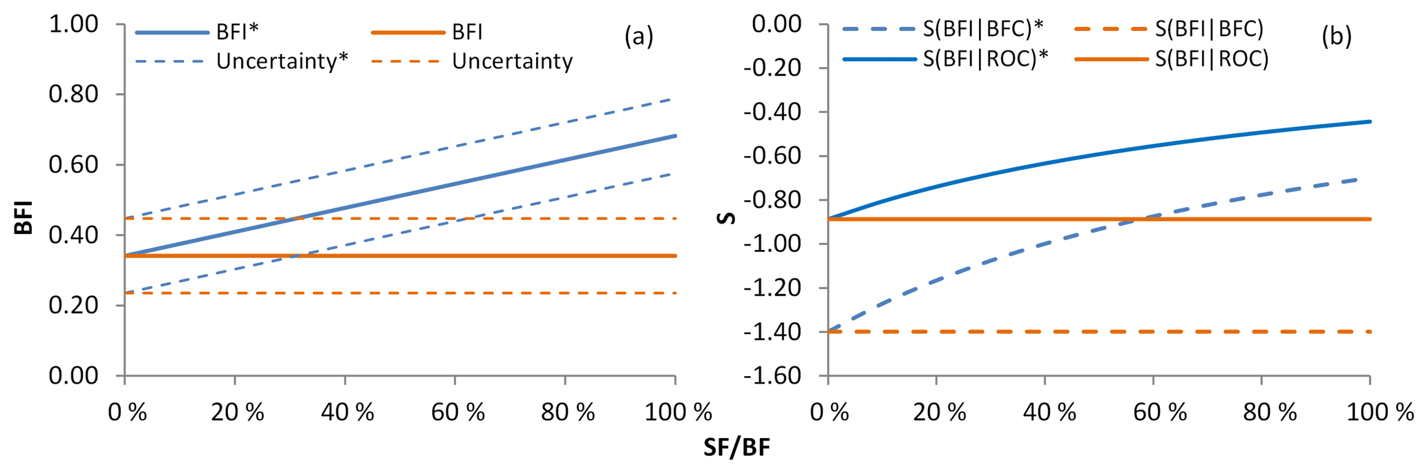
Figure 3Estimation results of (a) baseflow index and uncertainty (b) sensitivity indices, under different low-conductivity soil flow ratios, assuming high-conductivity baseflow remains unchanged. An asterisk indicates the results of the estimation considering the low-conductivity soil flow.
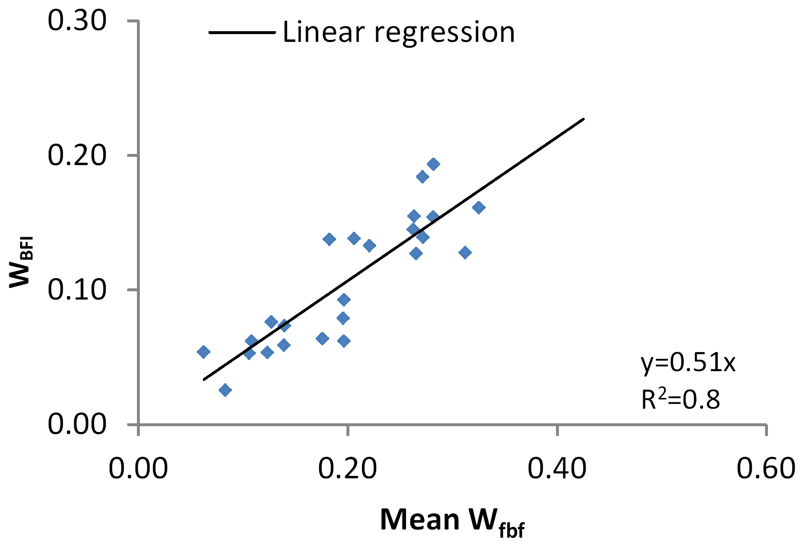
Genereux's method (Eq. 19) estimates the average uncertainty in BFI in the 24 basins (average of mean Wfbf) to be 0.20, whereas the average uncertainty in BFI (average of WBFI) calculated directly using the proposed method (Eq. 23) is 0.11 (Table 1). Mean Wfbf in each basin is generally larger than WBFI (WBFI is about 0.51 times of mean Wfbf), and there is a significant linear correlation (Fig. 2). This shows that the two methods have the same volatility characteristics for BFI uncertainty estimation, but Genereux's method (Eq. 19) often overestimates the uncertainty in BFI. This also means that when the time series is longer than 365 days, the measurement errors in conductivity and streamflow will cancel each other out and thus reduce the uncertainty in BFI (about half of the original).
The conductivity of shallow subsurface and soil flow in real watersheds is sensitive to climatic conditions and usually shows obvious fluctuations (Miller et al., 2014). The CMB method classifies high-conductivity flow (e.g., deep subsurface flow) as baseflow and low-conductivity flow (e.g., local shallow soil flow) as surface runoff (Cartwright et al., 2014). Therefore, in the watershed containing a large number of low-conductivity soil flows, the BFI calculated by the CMB method comprised only the baseflow index of the deep subsurface flow. The parameter sensitivity indices and uncertainty in the deep subsurface flow were also calculated by the methods of this paper. Cartwright et al. (2014) showed that the ratio of low-conductivity soil flow to high-conductivity subsurface flow in the Barwon Basin in southeastern Australia is close to 1. If only the BFI doubles and other parameters remain unchanged, then the sensitivity indices calculated by Eqs. (9) and (10) are halved, whereas the uncertainty calculated by Eq. (23) remains unchanged. Therefore, nonconstant soil flow conductivity may lead to an overestimation of sensitivity, but it has less impact on uncertainty estimates.
To better understand the effects of low-conductivity soil flow on BFI, parameter sensitivity, and the uncertainty estimation results, this study assumed that the high-conductivity baseflow is constant and the ratio of low-conductivity soil flow to high-conductivity baseflow (SF ∕ BF) is between 0 and 1. Based on the average values of the 24 watersheds mentioned in Table 1, the estimation results with and without consideration of low-conductivity soil flow were analyzed (Fig. 3). The CMB method used in this study neglects low-conductivity soil flow; thus, the BFI, sensitivity indices, and uncertainty do not change with a change in SF ∕ BF (orange line in Fig. 3). When the low-conductivity soil flow is considered in the estimations, the BFI value is found to increase linearly with the increase in SF ∕ BF (blue solid line in Fig. 3a); the absolute values of sensitivity indices decrease nonlinearly with the increase in SF/BF; and the difference between S(BFI|BFc) and S(BFI|ROc) decreases gradually (blue line in Fig. 3b). The uncertainty in BFI does not fluctuate with changes in SF ∕ BF (blue dashed line in Fig. 3a). In general, the deviation between BFI, sensitivity indices, and the “true values” gradually increases with an increase in the low-conductivity soil flow of a basin.
This study analyzed the sensitivity of BFI, calculated using the CMB method, to errors or uncertainties in the parameters BFC and ROC and the variables yk and SCk. In addition, the uncertainty in BFI was calculated. The equations derived in this study (Eqs. 9 and 10) could calculate the sensitivity indices of BFI for BFC and ROC. For time series longer than 365 days, the measurement errors in conductivity and streamflow exhibited a mutual offset effect, and their influence on BFI could be neglected. Considering the mutual offset, the uncertainty in BFI would be halved. From this perspective, Eq. (23) could estimate the uncertainty in BFI for time series longer than 365 days. The application of the method to 24 basins in the US showed that BFI is more sensitive to BFC. Future studies should dedicate more effort to determining the value of BFC. In addition, the CMB method may be more suitable for long time series of small watersheds.
Systematic errors in specific conductance and streamflow as well as temporal and spatial variations in baseflow conductivity may be the main sources of BFI uncertainty. Better rating curves are probably more important than better loggers, and understanding the specific conductance of baseflow is likely more important than understanding that of surface runoff.
The above conclusions were drawn only from the average of the studied 24 basins, and further research in other countries or in more watersheds is thus required. This study focused on the two-component hydrograph separation method with conductivity as a tracer, but parameter sensitivity analysis and uncertainty analysis methods involving other tracers are similar. Therefore, similar equations can easily be derived by referring to the findings of this study.
All streamflow and conductivity data can be retrieved from the US Geological Survey's (USGS) National Water Information System (NWIS) website using the special gage number: http://waterdata.usgs.gov/nwis (NWIS, 2018).
Because of n>0, BFI > 0 (BFC − ROC)>0, the above formula can be simplified:
Since BFC is usually much larger than SCk, the above formula can be rewritten as
The daily average streamflow () is usually much larger than 1 m3 day−1, so is far less than 1 day m−3.
The supplement related to this article is available online at: https://doi.org/10.5194/hess-23-1103-2019-supplement.
WY, CX, and XL developed the research train of thought. WY and CX completed the parameters' sensitivity analysis. XL completed the uncertainty estimate of BFI. WY carried out most of the data analysis and prepared the manuscript with contributions from all coauthors.
The authors declare that they have no conflict of interest.
This work is supported by the National Natural Science Foundation of China (41572216),
the Provincial School Co-construction Project Special – Leading Technology
Guide (SXGJQY2017-6), the China Geological Survey Shenyang Geological Survey
Center “Changji Economic Circle Geological Environment Survey” project (121201007000150012),
and the Jilin Province Key Geological Foundation Project (2014-13). We thank
the anonymous reviewers for useful comments to improve the manuscript.
Edited by: Markus Hrachowitz
Reviewed by: three anonymous referees
Cartwright, I., Gilfedder, B., and Hofmann, H.: Contrasts between estimates of baseflow help discern multiple sources of water contributing to rivers, Hydrol. Earth Syst. Sci., 18, 15–30, https://doi.org/10.5194/hess-18-15-2014, 2014.
Costelloe, J. F., Peterson, T. J., Halbert, K., Western, A. W., and McDonnell, J. J.: Groundwater surface mapping informs sources of catchment baseflow, Hydrol. Earth Syst. Sci., 19, 1599–1613, https://doi.org/10.5194/hess-19-1599-2015, 2015.
Eckhardt, K.: How to construct recursive digital filters for baseflow separation, Hydrol. Process., 19, 507–515, https://doi.org/10.1002/hyp.5675, 2005.
Eckhardt, K.: Technical Note: Analytical sensitivity analysis of a two parameter recursive digital baseflow separation filter, Hydrol. Earth Syst. Sci., 16, 451–455, https://doi.org/10.5194/hess-16-451-2012, 2012.
Ernest, L.: Gaussian error propagation applied to ecological data: Post-ice-storm-downed woody biomass, Ecol. Monogr., 75, 451–466, https://doi.org/10.1890/05-0030, 2005.
Genereux, D.: Quantifying uncertainty in tracer-based hydrograph separations, Water Resour. Res., 34, 915–919, https://doi.org/10.1029/98wr00010, 1998.
Hamilton, A. S. and Moore, R. D.: Quantifying Uncertainty in Streamflow Records, Can. Water Resour. J., 37, 3–21, https://doi.org/10.4296/cwrj3701865, 2012.
Huang, Z. P. and Chen, Y. F.: Hydrological statistics, China Water & Power Press, Beijing, China, 2011.
Kline, S. J.: The purposes of uncertainty analysis, J. Fluids Eng., 107, 153–160, 1985.
Lott, D. A. and Stewart, M. T.: Base flow separation: A comparison of analytical and mass balance methods, J. Hydrol., 535, 525–533, https://doi.org/10.1016/j.jhydrol.2016.01.063, 2016.
Mei, Y. and Anagnostou, E. N.: A hydrograph separation method based on information from rainfall and runoff records, J. Hydrol., 523, 636–649, https://doi.org/10.1016/j.jhydrol.2015.01.083, 2015.
Miller, M. P., Susong, D. D., Shope, C. L., Heilweil, V. M., and Stolp, B. J.: Continuous estimation of baseflow in snowmelt-dominated streams and rivers in the Upper Colorado River Basin: A chemical hydrograph separation approach, Water Resour. Res., 50, 6986–6999, https://doi.org/10.1002/2013WR014939, 2014.
Munyaneza, O., Wenninger, J., and Uhlenbrook, S.: Identification of runoff generation processes using hydrometric and tracer methods in a meso-scale catchment in Rwanda, Hydrol. Earth Syst. Sci., 16, 1991–2004, https://doi.org/10.5194/hess-16-1991-2012, 2012.
NWIS: US Geological Survey's National Water Information System, available at: http://waterdata.usgs.gov/nwis, last access: September 2018.
Okello, A. M. L. S., Uhlenbrook, S., Jewitt, G. P. W., Masih, L., Riddell, E. S., and Zaag, P.V.: Hydrograph separation using tracers and digital filters to quantify runoff components in a semi-arid mesoscale catchment, Hydrol. Process., 32, 1334–1350, https://doi.org/10.1002/hyp.11491, 2018.
Stewart, M., Cimino, J., and Rorr, M.: Calibration of base flow separation methods with streamflow conductivity, Ground Water, 45, 17–27, https://doi.org/10.1111/j.1745-6584.2006.00263.x, 2007.
Taylor, J. R.: An Introduction to Error Analysis: The Study of Uncertainties in Physical Measurements, Univ. Sci. Books, Mill Valley, Calif., 1982.
Wagner, R. J., Boulger Jr., R. W., Oblinger, C. J., and Smith, B. A.: Guidelines and standard procedures for continuous water-quality monitors-Station operation, record computation, and data reporting, US Geol. Surv. Tech. Meth. 1-D3, US Geological Survey, Reston, Virginia, 51 pp., 2006.
Zhang, J., Zhang, Y., Song, J., and Cheng, L.: Evaluating relative merits of four baseflow separation methods in Eastern Australia, J. Hydrol., 549, 252–263, https://doi.org/10.1016/j.jhydrol.2017.04.004, 2017.
- Abstract
- Introduction
- Sensitivity analysis
- Uncertainty estimation
- Application
- Conclusions
- Data availability
- Appendix A: Calculation of the partial derivatives
- Appendix B: Calculation of the sensitivity indices
- Proof that is far less than 1 day m−3
- Author contributions
- Competing interests
- Acknowledgements
- References
- Supplement