the Creative Commons Attribution 3.0 License.
the Creative Commons Attribution 3.0 License.
Passive acoustic measurement of bedload grain size distribution using self-generated noise
Teodor Petrut
Thomas Geay
Cédric Gervaise
Philippe Belleudy
Sebastien Zanker
Monitoring sediment transport processes in rivers is of particular interest to engineers and scientists to assess the stability of rivers and hydraulic structures. Various methods for sediment transport process description were proposed using conventional or surrogate measurement techniques. This paper addresses the topic of the passive acoustic monitoring of bedload transport in rivers and especially the estimation of the bedload grain size distribution from self-generated noise. It discusses the feasibility of linking the acoustic signal spectrum shape to bedload grain sizes involved in elastic impacts with the river bed treated as a massive slab. Bedload grain size distribution is estimated by a regularized algebraic inversion scheme fed with the power spectrum density of river noise estimated from one hydrophone. The inversion methodology relies upon a physical model that predicts the acoustic field generated by the collision between rigid bodies. Here we proposed an analytic model of the acoustic energy spectrum generated by the impacts between a sphere and a slab. The proposed model computes the power spectral density of bedload noise using a linear system of analytic energy spectra weighted by the grain size distribution. The algebraic system of equations is then solved by least square optimization and solution regularization methods. The result of inversion leads directly to the estimation of the bedload grain size distribution. The inversion method was applied to real acoustic data from passive acoustics experiments realized on the Isère River, in France. The inversion of in situ measured spectra reveals good estimations of grain size distribution, fairly close to what was estimated by physical sampling instruments. These results illustrate the potential of the hydrophone technique to be used as a standalone method that could ensure high spatial and temporal resolution measurements for sediment transport in rivers.
- Article
(4380 KB) - Full-text XML
- BibTeX
- EndNote


Sediment transport analyses in river catchments are one of the key activities stipulated by the European water framework directive (European Commission, 2001) and also applied in French environmental policies. Climate changes and anthropological actions impact the sediment transport in rivers such that it produces changes in the river morphology and may put at risk ecosystems and hydraulic structures, eventually. One of the major concerns of sediment transport in rivers is determining the total discharge of bedload transport (Gray et al., 2010). Bedload transport models are highly sensitive to incipient motion, which is directly related to river bed grain size distribution (GSD). Bedload GSD is linked to both surface and substrate GSD. In his paper, Parker (1990) constructed a two-size fraction transport model, assuming that the bedload GSD is identical to substrate GSD, for stable armored river beds, and becomes identical to surface GSD whenever the armor is destroyed. The development of surface-based and mixed-size transport models has received considerable attention (Heimann et al., 2015; Kuhnle, 1993; Parker, 1990; Recking, 2016; Wilcock and Kenworthy, 2002; Wilcock and McArdell, 1993). Knowing the bedload GSD solves the problem of initiation of motion and, therefore, enhances the accuracy of transport rate prediction. Therefore, measuring bedload leads to not only transport rates, but also to bedload GSD to calibrate models (Parker, 2002; Wilcock et al., 2009). However, obtaining bedload samples during exceptional hydraulic events may be difficult by using traditional bedload sampling techniques (e.g., pressure-difference samplers) (Bunte et al., 2010). To measure a wide range of discharge flows, the scientific community has been interested in developing indirect, or surrogate, methods that achieve continuous measurements no matter the hydraulic conditions (Gray et al., 2010; Hubbell, 1964). This paper is dedicated to the monitoring of bedload GSD using the acoustic noise naturally generated by bedload transport in rivers, the so-called bedload self-generated noise (SGN).
Acoustics surrogate methods are divided into two categories: active and passive methods (Gray et al., 2010; Hubbell, 1964). Examples of active methods are the acoustic Doppler current profiler, aDcp (Rennie and Millar, 2004), or the acoustic mapping velocity technique (Muste et al., 2016). Active methods use emissions of well-known signals but, actually, to the best of our knowledge, no active instrument was conceived to estimate bedload GSD. Besides, the major problem of the active instruments is that they do not properly behave during high flow discharges. This is why the passive instruments are preferred instead of the former. These instruments use seismic or acoustic signals generated by bedload particle impacts. Recorded signals contain information on both sediment impact rate and bedload particle sizes. One of the most widely used techniques consists in recording the signal of particle impacts on steel objects like plates (Rickenmann et al., 2014; Wyss et al., 2016a), pipes (Mao et al., 2016; Mizuyama et al., 2010) or column pipes (Papanicolaou et al., 2009). Other passive instruments consist in directly recording bedload SGN by using passive acoustic monitoring (PAM) (Barton, 2006; Bedeus and Ivicsis, 1963; Geay, 2013; Geay et al., 2017a; Thorne, 1986a, b) or seismic monitoring (Gimbert et al., 2014; Roth et al., 2016; Tsai et al., 2012). Measuring bedload GSD with passive methods has been achieved using plates (Barrière et al., 2015; Krein et al., 2014; Rickenmann et al., 2014; Wyss et al., 2016b) or pipes (Dell'Agnese et al., 2014; Mizuyama et al., 2010; Papanicolaou et al., 2009), and SGN (Geay et al., 2017a; Johnson and Muir, 1969; Jonys, 1976; Thorne, 1986a, b), by using experimental laws of calibration. Concerning seismic methods, bedload GSD measurements were not yet proposed as a direct application.
The existence of a link between the GSD and the features of vibrational signals has been demonstrated in several experiments (Belleudy et al., 2010; Bogen and Møen, 2001; Krein et al., 2008; Turowski et al., 2011). Coupling geophones with steel plates (Barrière et al., 2015; Wyss et al., 2016a) produced composite power laws by linking both peak amplitude and peak frequency to the grain size. Using the Japanese pipe, Mao et al. (2016) proposed an empirical model based on multi-channel recorded amplitude ratios to estimate different percentiles of grain diameters (D16, D50 and D84). The only metric exploited in this kind of measurement is the amplitude of shocks on steel structures. Thus, these passive techniques involving shocks on steel structures offer a high-quality signal, or signal-to-noise ratios (SNRs). The analyzed physics is the same as in the case of SGN measurements by PAM, which is the rigid body radiation caused by Hertzian impacts between sediments. In the case of SGN measurements, unlike the steel structure impact measurements, the SGN signal amplitudes are not usable for grain-size inversion because of the issues concerning the sound propagation throughout the reach (the amplitudes depend on the distance between the shocks and the hydrophone). This makes the amplitude a futile metric to infer grain-size information from SGN signals.
Several studies in the field highlighted that the frequency content (i.e., spectrum shape) of SGN signals is heavily dominated by grain sizes. For example, Jonys (1976) showed by laboratory experiments with ceramic spheres that spectral peak frequency is linked to sphere diameter. The author found a peak frequency at about 4 kHz for 19 mm diameter particles, at 2.2 kHz for the 38 mm diameter and at 1 kHz for the 75 mm diameter. This means that a doubling of grain size is almost equivalent to halving of peak frequency. Extensive research on GSD estimation by SGN recordings was done by Thorne (1986b), where he presented two strategies for inversion of acoustic spectra to estimate GSD. Results were encouraging as GSD was roughly estimated. These techniques are based on experimental measurements that have been made in a rotating drum with specific conditions that are different from the conditions found in rivers (e.g., impact velocities, acoustic propagation). Besides, his inversion techniques raise issues because of the broadband nature (shape) of spectra, even for uniform sediments. The author himself assumed that this was the major cause of inaccurate estimations of GSD from composite spectra.
This paper proposes an inversion method that solves the issue of spectrum shape and which accurately estimates the entire bedload GSD curve. This proposed method is conceived as being transferable to a large set of operational contexts. The procedure of inversion is based on a physical direct model which is presented in the first part of this paper. In the second part, the inversion algorithm is presented in the form of a technique for solving least square (LS) problems with a regularization condition about the positivity of the GSD curve. Simulated acoustic spectra and their inversion are used to test the robustness of LS methods to measurement uncertainties. In the third part, the LS inversion algorithm is applied to field measurements made in the large gravel-bed Isère River, France. GSDs estimated with our method are compared to GSDs measured with a pressure-difference sampler. Additionally, the cross-sectional variability of bedload GSD is analyzed using both acoustic and direct measurements. Finally, results are discussed to give a technical overview of the proposed inversion method.
2.1 Analytic model of Hertzian impact between a sphere and a slab
This section deals with spectral modeling of the impact between a sphere and a slab (Akay and Hodgson, 1978; Hunter, 1957), because the main assumption of this study is that the acoustics of gravel is described by impacts between bedload sediments and the river. To prove the validity of our model, the study includes some comparative facts with the sphere–sphere spectral model of Thorne and Foden (1988).
As a brief introduction, the collision between bed particles radiates energy. Such a rigid body radiation phenomenon is due to both vibrations and accelerations. These processes are very well separated with respect to their dominant frequencies, such that the spherical mode vibrations generate much higher frequencies than the acceleration-based sound (Barton, 2006; Thorne and Foden, 1988). The acoustic effect of accelerating rigid bodies is physically modeled by Kirchhoff (1883). A framework was constructed by Goldsmith (2003), Hertz (1882) and Hunter (1957) to model acceleration profiles from elastic impacts between two solid rigid bodies like two spheres or a sphere and a slab. In a mathematical sense, the acoustic pressure field generated from the acceleration of a rigid body is evaluated by the integral convolution from Eq. (1) (Akay and Hodgson, 1978; Koss and Alfredson, 1973; Thorne and Foden, 1988). The integral consists of the convolution between Kirchhoff's impulse response pI and an acceleration profile A. In the case of elastic (Hertzian) impacts the acceleration occurs during the impact, and so the integral is evaluated by intervals with respect to a contact duration Tc. The contact duration Tc is modeled by Hertz's law and it is put in a simplified form in Eq. (1), for both sphere–sphere and sphere–slab impact models.
where χ is the time interval of convolution, with χ=t, if 0 , and χ=Tc, if τ>Tc, with τ a delayed time due to sphere geometry, , r is the distance between the observation point and the impact (see also Fig. 1a and b), a is the radius of the sphere, c is the sound celerity, ρs is material density and Uimp is the impact velocity. The parameter ϑ(1) is a constant, ϑ(1)=9.229, for the impact between two spheres of the same radii and ϑ(1)=10.601, for the impact of a slab and a sphere. The parameter is a material parameter, and it contains Young's modulus (Elong) and the Poisson ratio (ν).
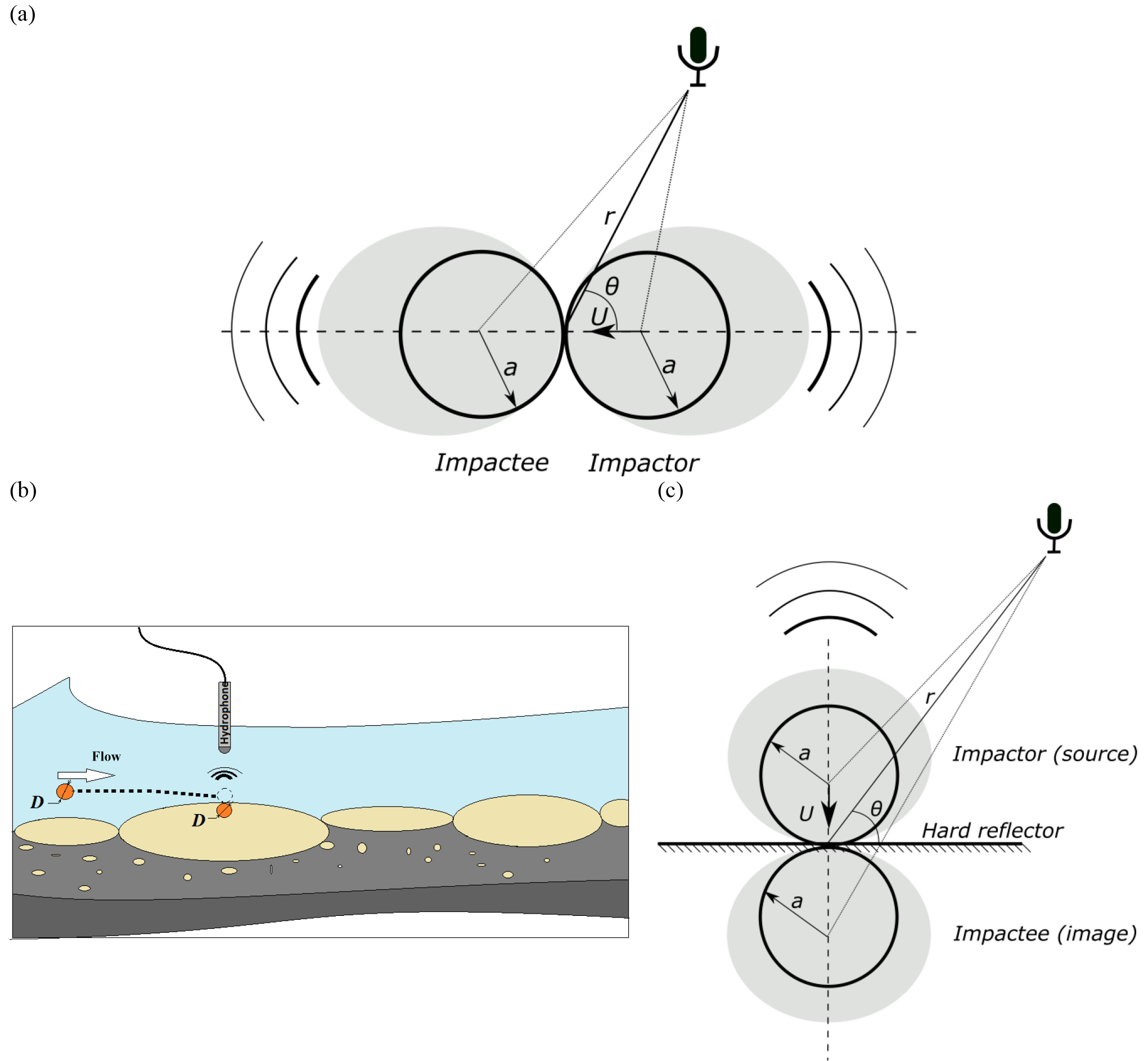
Figure 1(a) Setup for the impact between two spheres, here of the same radius a; the acoustic dipole source is illustratively depicted by the gray patch; (b) setup for the impact between a sphere of radius a and a semi-infinite rigid plane; to be noted is the boundary condition of the hard bottom (reflector) assumed in the framework of the “method of images”; thus, the impacting sphere is mirrored in the slab, so the acoustic fields are subtracted; the acoustic dipole source is illustratively depicted by the gray patch; (c) the elementary acoustic process of bedload noise in the river: the particle of equivalent diameter D=2a impacts the armored river bed (a massive slab) which generates a transient recorded by a hydrophone.
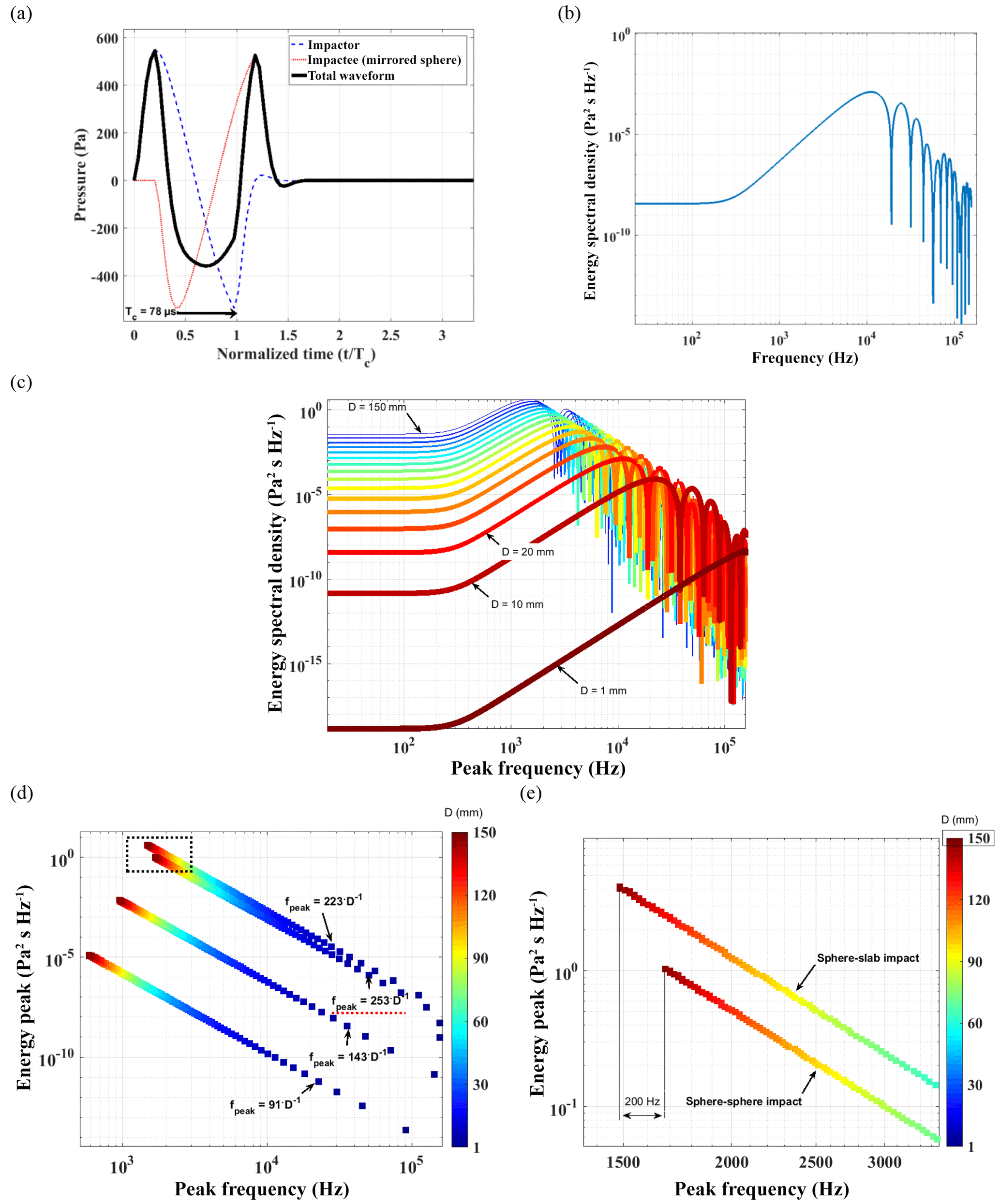
Figure 2(a) Analytical waveform of sound from impact between a granite sphere of diameter D=20 mm and a granite slab, where the impact velocity Uimp=1 m s−1, the directivity angle θ=0∘ and the sensor is r=1 m from the impact; the arrow indicates the contact duration Td; (b) the analytical spectrum modeled with Eq. (7) using the same parameters as in (a); the spectrum is an energy spectral density and is measured in Pa2 s Hz−1; (c) analytical spectra of sphere–slab impacts modeled by Eq. (7) as a function of diameter, mm; impact velocity Uimp=1 m s−1, the directivity angle θ=0∘ and the sensor is r=1 m from the impact. (d) Peak frequency fpeak and power peak variations, from spectra modeled by Eq. (7), with the diameter and the sphere's diameters; the diameters are coded by colors. The power law fpeak=aDb is given, where the sphere–slab impact tests consider three impact velocities () and the law of sphere–sphere impact is underlined by the dotted line; the material is granite. From bottom to top, the regression laws of sphere–slab impact vary from Uimp=0.01 (bottom) to Uimp=1 (top) m s−1. The sphere–sphere impact tests are done using Uimp=1 m s−1 and the same other parameters as with sphere–slab impacts. (e) Detail where the two vertical dotted lines locate the fpeak of the impact spectrum from 150 mm diameter particles for both impact models.
Table 1Parameters used to model analytical spectra of sediment size mixtures, Eq. (6b), and the typical values adapted for the underwater environment. The typical singular values are used in inversion further in this paper. The ranges of values are used in the global sensitivity analysis. K is the number of size classes used to inverse acoustic spectra.
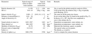
Table 2First-order sensitivity indices Si computed by the FAST method, assuming the peak frequency as the output of the model, fpeak: 0 % means no influence, and 100 % means total influence on the model output.
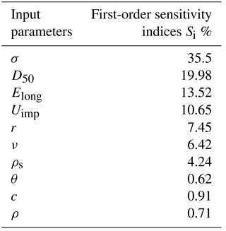

Figure 3GSA flowchart to compute the first-order sensitivity indices by the FAST method; the spectrum is simulated with Eqs. (7) and (6b), with a log-normal distribution generated using a diameter in the range 1 to 150 mm and SD σ in the range 0.01 to 10. The rest of the input parameters are defined in Table 1. From the simulated spectra, the fpeak are computed, and finally the first-order sensitivity indices Si are calculated using the FAST method. The results are shown in Table 2.
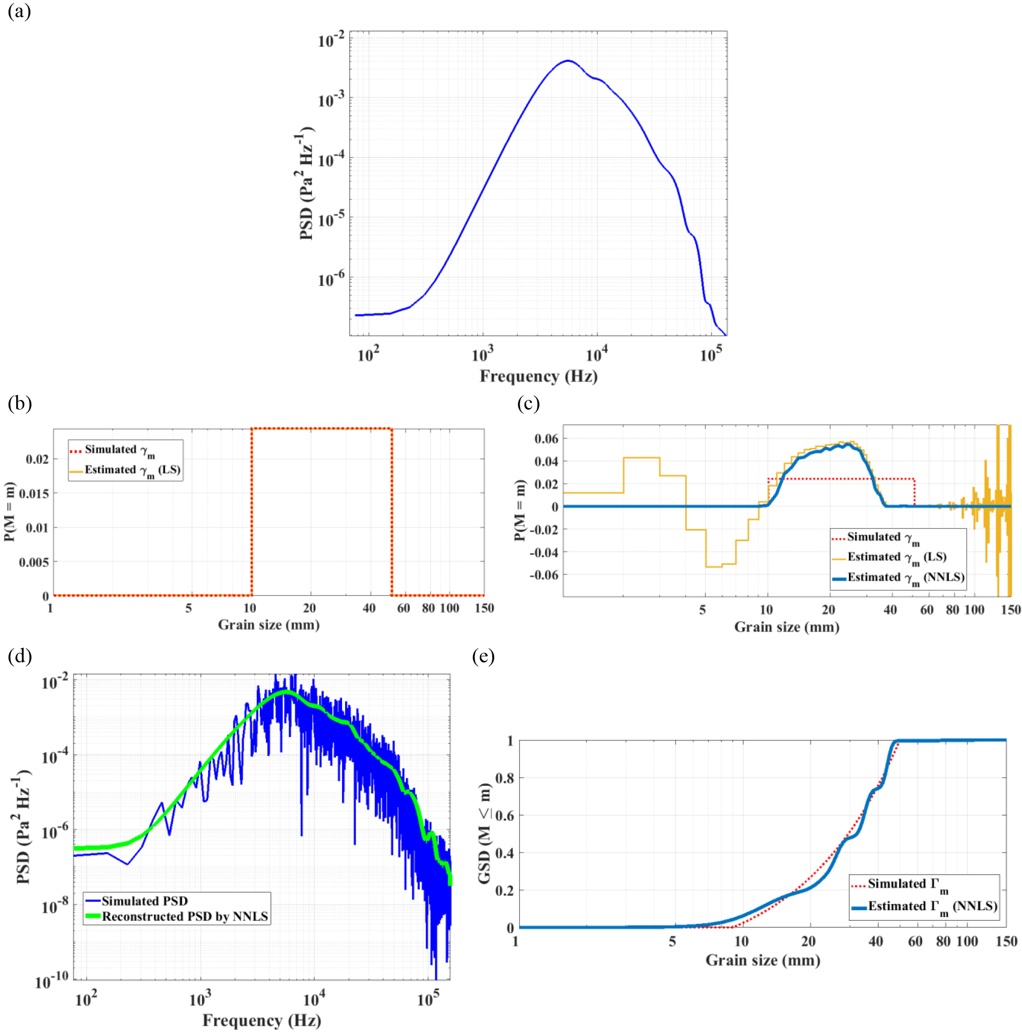
Figure 4(a) Simulated PSD from the uniform PMF γm of sediments, 10 kg per 1 mm size class, from 10 to 50 mm, where the impact velocity is Uimp=1 m s−1; the other input parameters are defined in Table 1; (b) the PMF solution obtained by the classical LS inversion, Eq. (12). The parameters used to simulate the PSD (grain size and impact velocity) shown in (a) are exactly the same as those used in modeling the dictionary Δ; (c) the PMF solutions obtained from the inversion of the spectrum shown in (a) using the two algebraic methods: the classical LS and the NNLS algorithm. The impact velocity used in modeling is Uimp=0.1 m s−1, whereas in the simulation it is Uimp=1 m s−1 (the other input parameters remain the same as in the simulation); the solution γm is post-processed by smoothing with a Gaussian moving window of 5 mm; (d) the simulated PSD shown in (a) with added variance (see text for the noise simulation procedure); (e) the cumulative GSD obtained from the inversion of the noised spectrum by the NNNLS algorithm. The estimated solution γ is used to reconstruct the spectrum, shown in green solid line in (d).
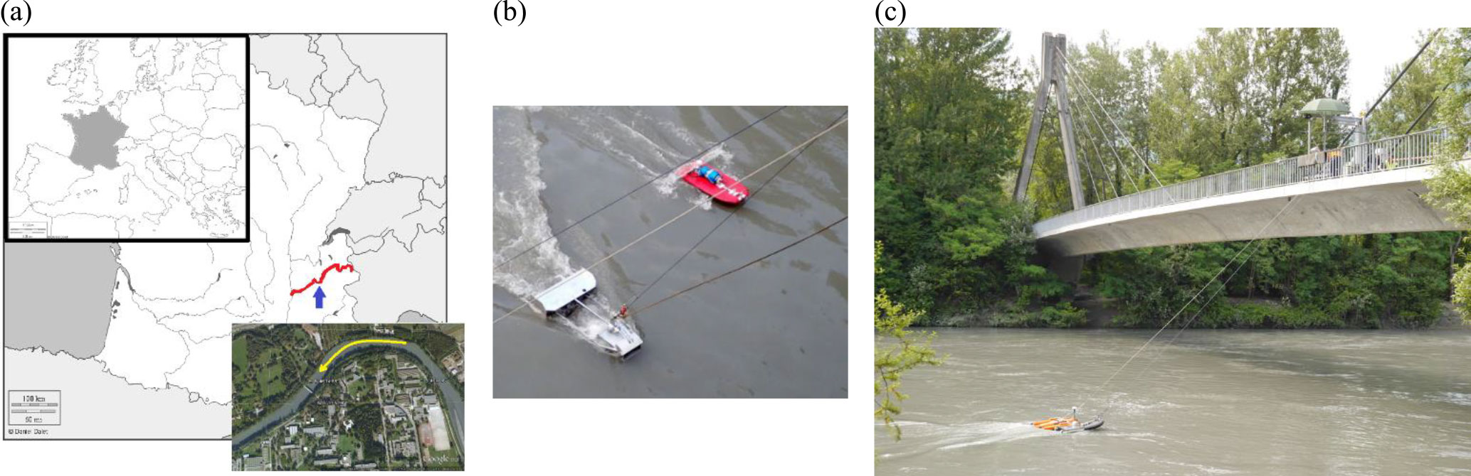
Figure 5Experimental setup: (a) Isère River basin geographical location (http://histgeo.ac-aix-marseille.fr) and Google Earth© picture showing the river morphology near the bridge where measurements were taken; (b) instruments used during the trials; from left to right: Toutle TR sampler and the floating river-board with hydrophone; (c) the bridge from where acoustic drifts and sediment physical samplings were realized.
The general form of the acceleration profile is provided by Goldsmith (2003) and it is rewritten in a unified form for both sphere–sphere and sphere–slab impact models; see Eq. (1).
where the constant ϑ(2)=1.5708, for sphere–sphere impact, and ϑ(2)=3.353 for sphere–slab impact.
The first important observation from Eq. (1) is the half-period sinusoidal form of the Hertzian acceleration. The two modeled acceleration laws show close frequencies as the constant ϑ(1) from Tc's formula is not dramatically different from one case to another. If the frequency of acceleration of sphere–sphere impact is 1000 Hz, then the frequency of acceleration of sphere–slab impact is 909 Hz, which is almost only 10 % of the deviation. The maximum amplitude of acceleration for the impact between two spheres of radius a is almost 2 times less than the impact between a sphere of radius a and a slab, considering the same Uimp and Tc.
The integral convolution in Eq. (1) is transformed into multiplication in the complex Fourier space. Thus, the analytical magnitude spectrum of the noise from the rigid body acceleration, Facc, is given in Eq. (4a).
where F(pI) is the Fourier transform (FT) of Kirchhoff's impulse response pI (Koss and Alfredson, 1973), for a sphere of radius a, defined in Eq. (4b), F(A) the FT of Hertzian acceleration due to elastic impact between two identical radii and the same material spheres, defined in Eq. (4c), and ω is the angular frequency which is a measure of rotation rate, in radians per seconds, and it is equal to 2πf; f is the linear frequency, a measure of number of occurrences per second.
j is an imaginary unit and for sphere–sphere impact, and ϑ(3)=1.067π2 for sphere–slab impact.
As we know, the nature of Hertzian sound is the oscillation of a rigid solid along a particular direction, and so each of the two objects in collision will give rise to a dipole acoustical source, shown in Fig. 1a. The case of sphere–slab impact is treated below. Hence, the amplitude of an oscillating sphere is dependent on the cos θ term and the phase of the acoustic pressure field changes by 180∘ at θ=90∘; i.e., the rarefaction wave changes into a compression wave or vice versa. In the case of the sphere–slab impact shown in Fig. 1b, the total pressure field is modeled as the addition between the compression wave and the slab-reflected rarefaction wave of the acoustic dipole. Thus, the addition becomes a subtraction as the reflected rarefaction wave keeps its sign (does not shift in phase), so there are two waves (compression and rarefaction) arriving at the sensor almost at the same time (Akay and Hodgson, 1978). This acoustic process is modeled by the so-called method of images by which one considers a mirrored sphere replacing the slab and being responsible for the rarefaction wave generation.
The same subtraction is applied in the case of complex spectra to obtain the total spectrum Fim, Eq. (5). In this formula, the first term of the right member is attributed to the impacting sphere, whereas the second term pertains to the mirror. The time delay Td of sound arrival due to distance of measurement and the sphere's geometry make the two terms not perfectly cancel out or not arrive at the same time at the sensor.
Introducing Eqs. (1), (1) and (4a–c) into Eq. (5), one obtains the complex magnitude spectrum of the impact between a sphere and a slab. The spectrum contains complex numbers, so one applies the multiplication of the spectrum and its conjugate to compute the magnitudes of the energy spectrum, Eq. (6).
where is the complex conjugate of Fim.
The quantity from Eq. (6) is noted as in Eq. (7) by E and its unit of measurement is Pa2 s Hz−1. Thus, the analytical model of impact used in this paper is an energy spectral density and it will be used to inverse acoustic spectra measured in the field.
An example of an analytical model computed in time by Akay and Hodgson (1978) and reformulated in Appendix B is presented in Fig. 2a. The impacting sphere is 20 mm in diameter, the material is granite and the impacting velocity is 1 m s−1. The shape of the waveform is an approximately one and a half period sinusoid. The subtraction of the two pressure fields, the rarefaction and the reflected compression wave fields are observed. It is also important to notice that the first arrival at the sensor is the compression wave. Thereafter, the other part of the acoustic dipole (the rarefaction wave) arrives with delay Td at the sensor. The power spectrum density modeled by Eq. (7) is shown in Fig. 2b. Here, the spectrum has a principal lobe and numerous side lobes. The principal lobe has a peak at the frequency of approximatively and the side lobes are approximatively associated with the term cos (ωTc) also observed by Thorne and Foden (1988).
In Fig. 2c it is shown that the frequency peaks of spectra from both types of impact model decrease with the sphere's diameters (from 1 to 150 mm), as experimentally observed by Thorne (1986b). Frequency peak as a function of diameter D, in the case of sphere–slab impact, , is given in the case of three impact velocities, . The exponents of the regression laws prove the exact inverse proportionality between fpeak and D. Besides, the power peaks and peak frequencies increase, for a certain diameter, when the impact velocity increases. There is only a doubling of fpeak when Uimp changes by an order of magnitude. This is also proved by the formula of Eq. (1) of Tc (almost the reciprocal of fpeak) where the parameter Uimp is raised to a weak exponent of −0.2.
The fpeak in the case of sphere–sphere impact, modeled for impact velocity Uimp=1 m s−1, is higher than in the case of the sphere–slab impact. Here, the analytical model of the sphere–sphere spectrum was computed using Eqs. (4a) and (5), with the two pressure fields auditioned instead subtracted. This gives the same results as the spectral model reported by Thorne and Foden (1988). To give an idea, a 150 mm diameter particle in sphere–sphere impact has a spectrum of fpeak=1700 Hz (see detail of Fig. 2c), whereas sphere–slab impact has fpeak=1500 Hz, so the 200 Hz represents cca. 15 % of variation between the cases.
It is worth mentioning that Uimp greatly influences the power peak, if the former is changed by 1 order of magnitude. On the other hand, the power peak of the sphere–sphere impact is slightly weaker than the sphere–slab impact. In this paper, we choose to use a slab model to model bedload SGN as it simplifies the inverse problem. Indeed, the task of determining the dimensions of impacted particles is skipped. Therefore, we consider that the riverbed could be modeled as a slab. This hypothesis could be supported when the riverbed is armored or paved, but may be false when the riverbed is totally mobile and when the impacts between particles of different diameters are very common.
2.2 PSD model of the SGN generated by a mixture of sediments
In the previous section, the analytic energy spectral density (ESD) was defined for the impact between a sphere and a slab. In this section, we model the power spectral density (PSD) of a sediment mixture using these analytic ESDs and the impact rate of each class of diameter, or the number of impacts per second. Assuming that particle collisions are random and independent noise sources, the model of the PSD of a mixture, denoted by P, can be expressed as a linear summation of the elementary ESD, denoted by Ei (Johnson and Muir, 1969; Jonys, 1976; Thorne, 2014) weighted by the impact rate Ii. The acoustic bedload model under discussion is defined in the scalar form in Eq. (6) and the matrix form in Eq. (6a).
where Δ is the dictionary of elementary ESD of impacts between spheres and slab and I is the vector of impact rates per diameter class or, basically, a histogram. Class i takes integer values, from the lowest limit, 1 mm, to the highest one, K mm, where K is the largest diameter considered in modeling. Here, we consider K equal to 150 mm. The parameter NFFT is the number of values contained in the spectrum or the number of Fourier transform points on which the spectrum is modeled.
The histogram I can be transformed in the probability mass function γ by normalizing it by its sum of elements. The cumulative form of γ will be denoted by Γ. Thus, one of the main assumptions is that Eq. (6a) can be written in terms of probabilities γ, as in Eq. (6b):
where γi represents the probability of having a number of impacts of particles per second for size class i.
Therefore, the random variable here is I and γ is the probability of impacts, and so the quantity γ (I=Ii) is a discrete probability, given that we operate on size classes of 1 mm in diameter. This probability is computed from a histogram of the number of impacts per second, so one needs to transform it into a histogram in mass of sediments M, to be compatible with the measured GSD by physical sampling. In consequence, γ (I=Ii) will be scaled by , as in Eq. (7), in order to obtain γm(M=mi). Finally, the grain size distribution (GSD), or the cumulative distribution form of γm, will be Γm(M≤mi), expressing the probability of sediments finer than Di, as defined in Eq. (7).
where Di is the diameter in meters and κ is a constant which is the rest of the mass-volume formula coefficient including the material density.
This section gave a formal definition of the PSD of a bedload size mixture defined by its GSD. The proportions are considered to be a probability mass function (PMF) of the rate of impacts. The size classes concerned in this study are integer numbers, from 1 to K, with a resolution of 1 mm per size class.
2.3 Global sensitivity analysis of the spectrum generated by a mixture of sediments
This analysis was done to determine the importance of input parameters for the shape of the PSD modeled with Eq. (6b). The parameters are defined in Table 1. Global sensitivity analysis (GSA) is done to assess the impact of input parameters on the model output, which in our case is the peak frequency fpeak of spectra modeled by Eq.(6b). We use the Fourier amplitude sensitivity test (FAST) (Cukier et al., 1973) to compute the first order indices of sensitivity Si for each input parameter. The coded version of the FAST algorithm is presented in Cannavó (2012).
The flowchart of the GSA is presented in Fig. 3. The FAST analysis uses the typical range of parameters found in rivers, defined in the second column of Table 1. The input log-normal distributions (GSD) have median diameter values in the range from 1 to 150 mm and SDs σ from 0.01 to 10. All other input parameters needed for the model in Eq. (6b) are given in Table 1. As the output model analyzed is the peak frequency fpeak of the simulated PSD curves, the analysis does not claim to completely describe the model, but pertinent ideas could be drawn on the model's behavior.
The results in terms of first-order indices are presented in Table 2. The SD σ of log-normal GSD has the greatest influence on the PSD shape. This is because σ affects the values of all percentiles of the GSD curve. The median D50 is almost 2 times less important than σ. The third-greatest parameter as a degree of influence on output is surprisingly Young's modulus, but this is due to a very wide range of values (here Pa, i.e., from quartz to granite materials). Such variation is not possible at the reach scale, where the sediments are of the same material. The impact velocity Uimp comes shortly after Young's modulus and confirms the conclusion of the previous local analysis, that Uimp has ca. 10 % of importance in the output. Other relatively important parameters are Poisson's ratio and the density of sediments, which means that the type of material also plays a role in the dynamics of the fpeak. The distance of measurement, r, also plays also a role in the fpeak variation. The angle of the point of observation with respect to the impact, θ, and the propagation medium properties, ρ and c, are considered of little influence on the values of fpeak.
In conclusion, the first-order global sensitivity analysis of the peak frequency shows a comprehensive view of its dynamics with input parameter variation. It is found that the peak frequency is mainly affected by two parameters, the distribution's SD and the median diameter, together making up ca. 65 % of output variation, whereas the material properties (i.e., density, Poisson's ratio, Young's modulus) have almost ca. 20 %, and the impact velocity Uimp has ca. 10 %. In conclusion, the acoustic model is quite complex and care must be taken regarding the recording of the power spectra on the field, as their shape heavily affects the estimation of GSD. Also, the impact velocity is regarded as a minor factor of uncertainty and, because it is almost impossible to be measured for each grain size class, the 10 % uncertainty in peak frequency is almost unavoidable. The material properties should not be a problem with the condition that the sediments are the same. For a complete GSA, the computation of high-order sensitivity indices can be made using Sobol's methodology (Sobol, 2001), but this type of analysis is beyond the scope of this article.
2.4 Assumptions on the proposed SGN spectrum model
Modeling of single impacts requires definition of parameters typical for river environments, in Table 1. Using the global sensitivity model, it has been shown that PSD shapes are essentially influenced by four parameters: the shape of the GSD curve, the median diameters of the colliding particles, the impact velocities and the material. Grain sizes are estimated later using the inversion algorithm presented in Sect. 3. Concerning the other model parameters, as they do not affect the PSD shape, they will be fixed for the inversion process, using realistic values. These parameters are listed in the third column of Table 1. The main assumptions of the SGN spectrum model are the following.
- i.
The geometry of the channel and of the material: the river bed is considered a massive slab and moving particles are considered spherical.
- ii.
Sediment transport assumptions: impact velocities are assumed to be invariant with grain size. This assumption is supported by the relative size effects on bedload transport (Einstein, 1950; Recking, 2016; Wilcock and McArdell, 1993) referring to the mobility of finer and coarser particles.
- iii.
Acoustic propagation:
-
as the bedload GSD is assumed to be homogeneous everywhere in the space, the propagation effects like the attenuation with distance (geometrical spreading models) will not impact the spectrum shape;
-
the attenuation due to diffraction from bed and water surface roughness or from the suspended sediments is not considered. The issue of the nonlinear propagation will be detailed in the discussion part of this paper.
-
The inversion uses least square (LS) optimization methods to compute the inverse of dictionary Δ. Normally K<NFFT, so Δ is a non-square matrix. Moreover, the matrix Δ is possibly rank deficient because the spectra generated by impacts of coarser particle sizes show very similar shapes, that is, the coarser the particle, the more similar the produced sound. This is also shown in Fig. 2b, where one could observe that the points on the graph agglomerate as the grain diameters increase. In this case, the pseudo-inverse algorithm is used to solve the algebraic system of Eq. (6b). The optimization problem is defined as in Eq. (12). The least square solution to this problem is the PMF of the rate of impacts γ. The estimated PMF is further transformed into the final GSD of mass of sediments according to Eqs. (7)–(7).
where is the pseudo-inverse, and Δt means the transpose of the matrix Δ.
Eq. (12) conveys the idea of minimizing the error between the model and the measurement. This minimization operation is realized in the sense of the least square optimization.
3.1 Numerical test of the LS method
A simulation case is proposed here to test the robustness of the LS inverse method. The simulated PMF, or grain size distribution, γm is uniformly distributed between 10 and 50 mm. The uniform distribution means that 1 kg of D=10 mm has the same probability of producing impact noise as 1 kg of D=11 mm, and so on. To obtain γ, the simulated PMF γm is converted back to impact rates by dividing by D3, D in meters. Using an impact velocity of 1 m s−1 and the rest of the input parameters defined in Table 1, the simulated PSD P is shown in Fig. 4a. Here, the dictionary Δ contains spectra from 1 to 150 mm and the grain size distribution has 1 mm resolution. Applying Eq. (12) on the simulated spectrum and considering exactly the same parameters in modeling and in simulation, it is found that the estimated γm is exactly the same as the simulated γm, as is expected; see Fig. 4b.
However, if the impact velocity used in modeling the dictionary is set to a value (Uimp=0.1 m s−1) which is different than the one used in simulation (Uimp=1 m s−1), then high instabilities are observed on the estimated γm; see Fig. 4c. This is explained by the fact that there is a high similarity between the elementary spectra E, especially for the larger size classes. Thus, the matrix Δ is ill-conditioned and the problem is ill-posed. Ill-conditioning is linked to the high condition number of the normal matrix (Δt.Δ). It is defined as the ratio between the largest and smallest eigenvalues of a matrix. A well-conditioned algebraic system requires that the normal matrix should have a condition number as close as possible to 1 (Strang, 2006). In these tests, Δ's condition number reaches huge values on the order of 1012–1020. In consequence, the similar spectra from the matrix Δ produce high instability in solution.
To avoid the instability in the LS solution, the non-negative least squares (NNLS) algorithm (Lawson and Hanson, 1974) is proposed to solve the LS problem. This optimization algorithm, Eq. (13), casts non-negative constraints on solution γ. The non-negative factorization is widely used, for example, in various domains like image processing or chemometrics. The side-effect of using this algorithm is the strong regularization of solutions. The regularization aims to keep the sum of components in γ constant. The solution of the NNLS algorithm (see Fig. 4c) shows that the instabilities are completely removed off. Besides, it is important to note that the estimated diameters are inside the simulated interval of diameters.
3.2 Robustness of the NNLS algorithm to PSD noise
The signal processing tools in this paper refer to using the PSD as the method of spectral representation of bedload signal. The use of PSD is worthwhile because the type of bedload signal is a stationary random one. Random stationary signals are signals varying in time but whose average and SD of amplitude values over some fixed periods are constant.
A particular concern for the signal processing of random processes is the minimization of the variance on the PSD. This work makes use of the periodogram algorithm for the PSD estimation, which means the Fourier transform is applied on local portions (windows) of the random signal, with an overlap of 50 %, and then the local results are averaged in narrow bandwidths (Oppenheim and Verghese, 2010). The averaging is useful because it mitigates the variance on the PSD. In this work, the quality of spectra is vital for accuracy of estimations. The uncertainty principle tells us that the smaller the temporal window, the greater the uncertainty in locating two very close frequencies on the spectrum, so a trade must be made between the PSD variance and its spectral resolution. If the bedload signal is too short, the quality of spectra toward the low-frequency bands is worsened because in one single bandwidth of the Fourier transform there is spectral information of impacts from multiples grain sizes. Finally, the longer the signal the better the spectral resolution and the less the variance on the PSD curve.
The NNLS algorithm will be tested on three simulated spectra which have different degrees of variance. The simulated γ used is identical to that in Sect. 3.1. The simulated signal is obtained by convolving a realization of a white noise with a transfer function being the modeled spectrum shown in Fig. 4a. The simulated noised PSD is shown in Fig. 4d. The results of the inversion using the NNLS algorithm show that, even for the worst scenario of variance on a spectrum, the inversion method correctly reconstructs the simulated GSD; see Fig. 4e.
Finally, we conclude that the NNLS algorithm is robust with respect to PSD noise and fits to this kind of inversion problem. The inversion procedure will now be tested on in situ measurements.
4.1 Isère River and experimental setup
The Isère River is a piedmont gravel river bed located in southeastern France, and it is one of the main tributaries of the Rhône River, which reaches the Mediterranean Sea. The monitoring section is located in the city of Grenoble (45∘11′52.8′′ N, 5∘46′14.88′′ E); see Fig. 5a. In this reach, the mean slope is about 0.06 %, the area of the watershed is 5500 km2 and the annual average flow rate is 180 m3 s−1. At the time of experiments, 29–30 June 2016, the monitored discharge was on average 300 m3 s−1. The measurement section has a rifle-pool morphology with riprap-protected embankments. Two different types of instrument were used: SGN measurements using hydrophone and direct sampling using a pressure-difference sampler, shown in Fig. 5b. All these measurements were carried out from a suspension bridge (Fig. 5c).

Figure 6(a) Positions of the floating board during drift experiments, with essential positions marked on the bridge, X= {14, 35, 58} m across the river; (b) the PSD estimated from the 12 drifts, in units of Pa2 Hz−1; to be noted is the change in peak frequencies: the leftmost position (Drift no. 12) has the highest frequency, meaning that the finer size fractions are transported, and the particles are getting coarser up to the right bank; (c) the measured SPL map from the 12 drifts, in units of dB re 1 µPa; the maximum values are found in the middle of the Isère River's cross section.
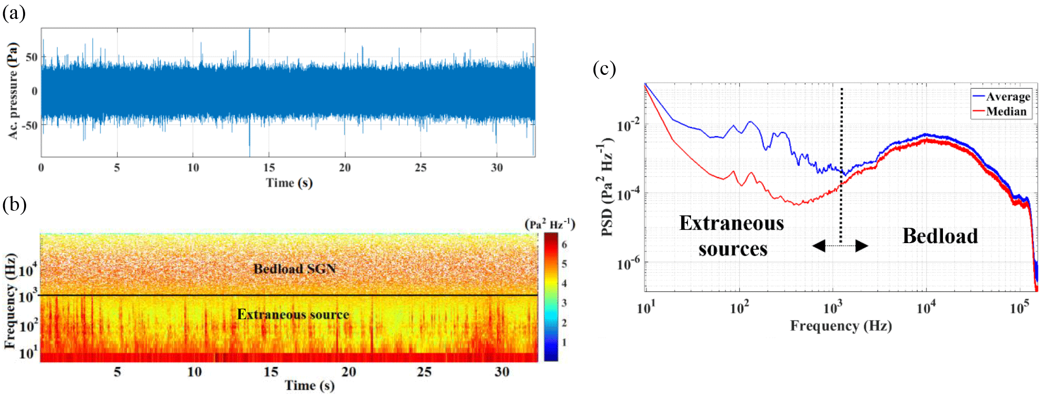
Figure 7Signal representations of the SGN recorded during hydrophone experiments on the Isère River (France): (a) temporal signal in units of Pa; (b) time–frequency representation (spectrogram), with the color code normalized with respect to power values, in Pa2 Hz−1; the specific frequency bandwidth of the bedload acoustic effects and of the hydrodynamic noise agitation (extraneous sources) are indicated; (c) the PSD curve, also in Pa2 Hz−1, estimated using either the average or the median power values, in time, from the spectrogram in (b).
4.1.1 SGN measurements
SGN measurements were made using a HTI99 hydrophone (High Tech, Inc., http://www.hightechincusa.com/) with a sensibility of −160 dB re 1 V µPa−1 ± 3 dB from 10 Hz to 125 kHz. The hydrophone was connected to an autonomous-waterproof autonomous recorder – SDA14 (RTSYS©, http://www.rtsys.eu). The gain of the recorder was set to 15 dB. Signals were sampled at a 312 kHz frequency with a resolution of 24 bits and saved as wav files. The scope of these field experiments was to trace maps of the SGN on the local reach. The hydrophone and the recorder were attached to a free-floating river-board. The hydrophone position was about 1 m below the water surface and 1.5 m on average above the river bed. The SGN map consists in launching 12 drift measurements from the bridge which are located due to a GPS device connected to the acoustic recorder. Each drift consists of recordings of about 30 to 40 s, or in terms of distance, between 50 and 100 m. The river-board positions during the drifts are shown in Fig. 6a. The recorded signals were processed to compute acoustic spectra. The 12 acoustic spectra recorded across the river (Fig. 6b) are inversed to estimate the bedload. The river cross section is about 60 m. Also, the 12 drift measurements are synchronized with GPS data to compute the SGN map in terms of sound pressure level (SPL), as is shown in Fig. 6c. The variability of SGN noise from the left to right banks can be observed from both the spectra and SPL map.
4.1.2 Definition of the SGN spectrum
SGN signals are measurements of bedload transport noise propagating in the river environment. Several representations of the acoustic signal are presented hereby, computed on the signal recorded in the middle of the Isère River (X=34 m): (a) the temporal waveform, in Fig. 7a; (b) the spectrogram, in Fig. 7b, as the scaled squared magnitude of short-time Fourier transform, in Pa2 Hz−1; and (c) the PSD, also expressed in Pa2 Hz−1, computed by either averaging or medianizing the PSD spectrogram, in Fig. 7c. Two main sources of noise can be distinguished in the recordings: below and above 400 Hz (Fig. 7). Bedload impacts can clearly be heard in the higher frequency band, sounding like the crackling of flames. Sounds occurring below 400 Hz are non-propagating sounds as they are localized below the cutoff frequency of the river waveguide (Geay et al., 2017b; Rigby et al., 2016). They are related to turbulence-induced noise around the sensor and to mechanical movements of the structure sharing the hydrophone. In the Isère River experiment, the SGN signal measured by drifts is almost free of hydrodynamic noise, which is proved by the typical median spectrum presented in Fig. 7c. In this study the inversion will be applied on such high signal-to-noise ratio PSD curves.
The median procedure is used to provide better smoothing as it filters more efficiently the unwanted low-frequency noises (Geay et al., 2017a). As in Fig. 7c, the suppression of the lower-frequency spikes can be noticed, attributed to the hydrodynamic noise, when median PSD is used instead of the average one.
4.1.3 Pressure-difference sampling
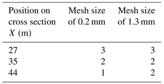
A Toutle River (TR) sampler, depicted in Fig. 5b, has been used to sample bedload particles (entrance width of 305 mm by 152 mm). There were two mesh sizes used for sampling: 0.2 and 1.3 mm. Sample durations were between 4 and 8 min. Finally, each bedload sample was dried, weighted and sieved in the laboratory. The sampled sediments were classified into six size classes: K= {<0.5; 0.5–2; 2–8; 8–16; 16–32; 32–64} mm. The TR sampler has been deployed in three cross-sectional positions (at X=27 m, X=35 m and X=44 m, marked on the bridge from the left to right river banks). The number of repetitions for each cross-sectional position is indicated in Table 3. Bedload fluxes () have been averaged for each position of the sampler. GSDs have been computed for each position and for each mesh size used.
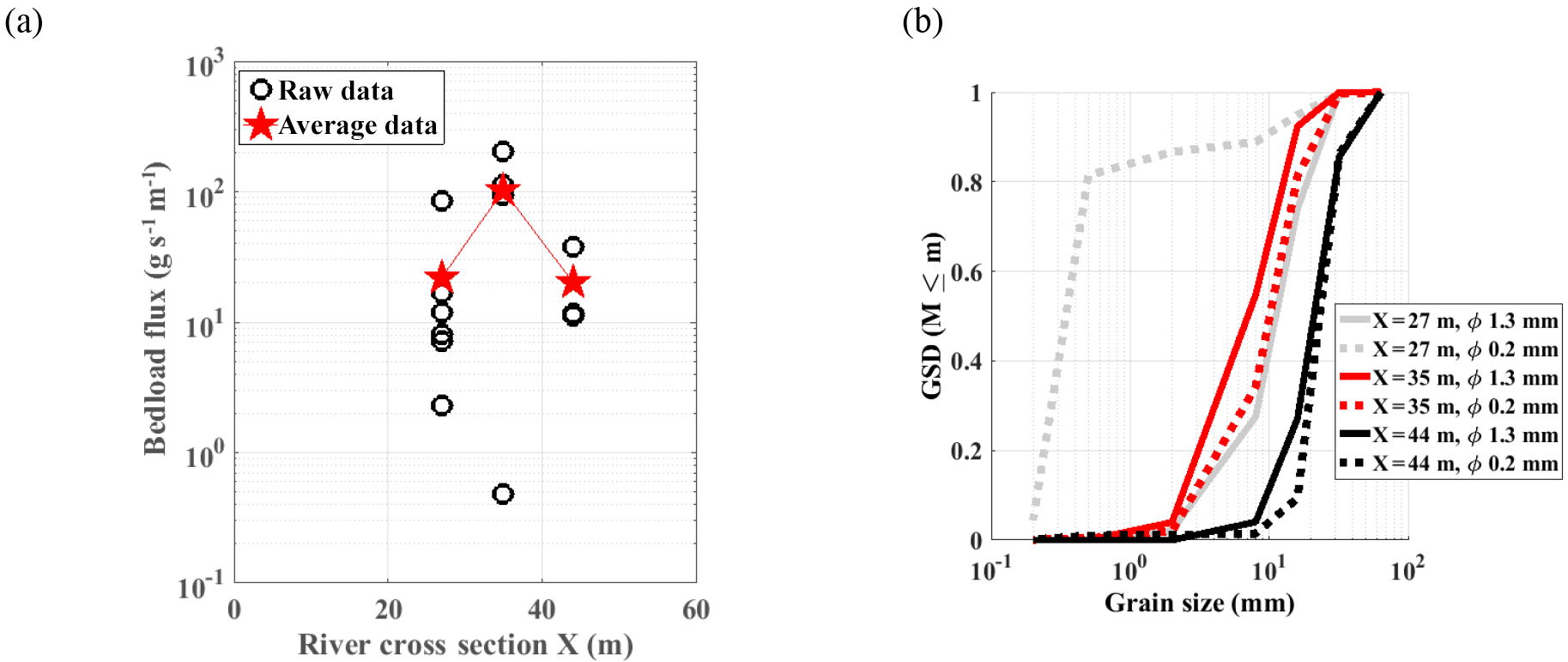
Figure 8Measured bedload flux in three positions across the Isère River, and (b) measured GSD curves in these positions, using the TR sampler with two mesh sizes, 0.2 and 1.3 mm.
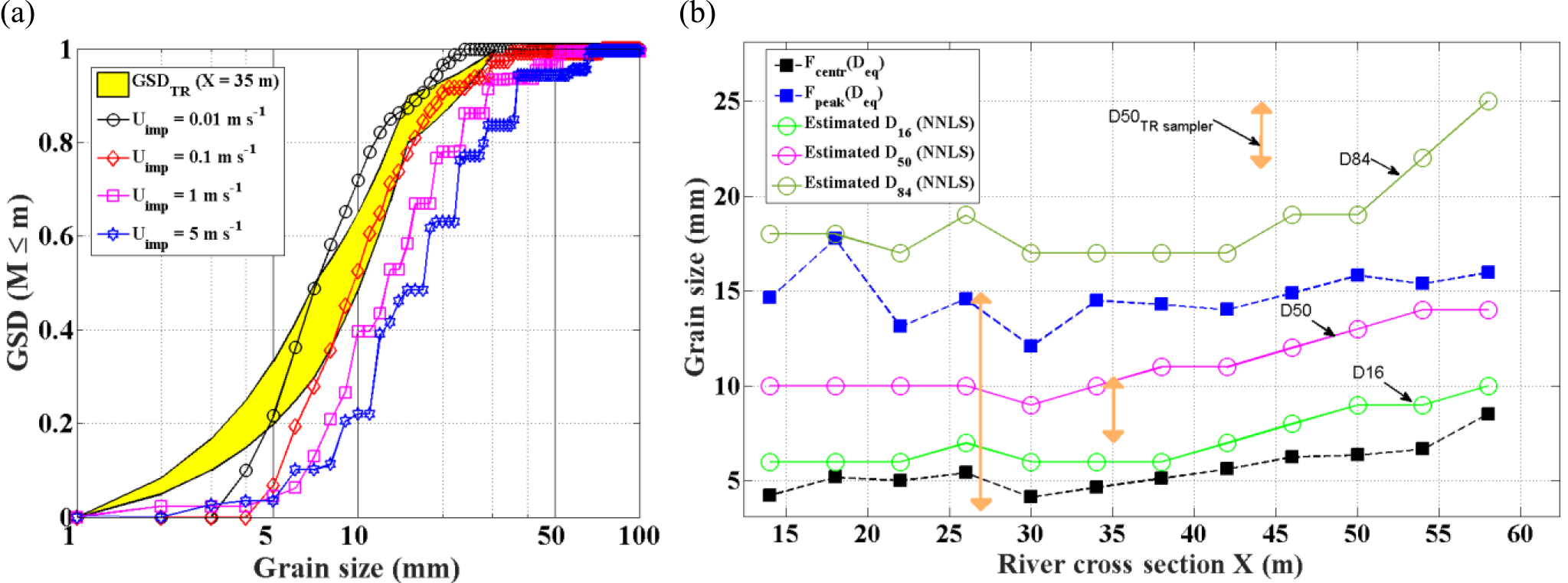
Figure 9(a) Estimated GSD by the NNLS algorithm in the center of the Isère River (X=34 m), using different values of impact velocities Uimp= {0.01, 0.1, 1, 5} m s−1. Measured GSD by TR sampler (X=35 m) is represented by the yellow envelope for the two mesh sizes (see Fig. 9b for fraction sizes finer than 1 mm); (b) The D16, D50, and D84 estimated by NNLS across the Isère River compared to the regression laws of Thorne (1985, 1986b) for estimating the equivalent diameter Deq; we also indicate by arrows the range of D50 measured by the Toutle River sampler (in positions ). The impact velocity used in the inversion is Uimp=1 m s−1.
4.2 Results
4.2.1 Direct measurements of bedload
Results of TR sampler measurements are shown in Fig. 8a–b. A maximum of bedload flux was found in the middle of the cross section (X=35 m) (Fig. 8a). A value of 100 has been measured. In side positions, the flux was found to be 5 times smaller, around 20 . Concerning grain size distributions, most of the measurements indicate a D50 between 7 and 20 mm. Notice that measurements made with the 0.2 mm mesh size towards the left bank (X=27 m) indicate a GSD toward much finer sediments (D50 of about 0.3 mm) (Fig. 8b). Bedload samples closest to the left bank were indeed constituted of huge amounts of fine sediment mixed with vegetable debris (about 60 % of the total mass sampled). In the central and right positions, neither vegetable debris nor silts were sampled. TR sampler measurements showed grain size sorting along the river cross section, varying from silts, near the left bank, to gravel, near the right bank.
In the following, the GSD measured in the central position (X=35 m) will be considered. Its flux was indeed the largest measured, and it is considered to be the principal source of bedload noise throughout the river.
4.2.2 SGN spectra inversion
All the median PSDs of SGN signals recorded across the Isère River have been presented in Fig. 6b. The seventh drift will be studied, the one positioned in the center of the cross section at X=34 m, which is the closest to the middle position of TR sampling measurements. In this position, it can be observed that a maximum bedload acoustic energy has been recorded. Additionally, a maximum flux of sediments was sampled in this position. The results of spectrum inversion, using a modeled dictionary Δ with size classes from 1 mm to K=100 mm (100 size classes), are shown in Fig. 9a. The results are compared to the GSD measured by the TR sampler in position X=35 m. Four different values of the impact velocity Uimp are tested (from 0.01 to 5 m s−1) and it is noticed that the impact velocity Uimp between 0.01 and 0.1 m s−1 leads to a very good match between estimation and TR sampling measurements, except for the very small size classes from 1 to 5 mm. The value of impact velocity Uimp=0.1 m s−1 will be used in the inversion of all other spectra measured across the Isère River.
Secondly, the GSD variations, represented by the percentiles D16, D50 and D84, are estimated by the inversion of 12 drift measurements taken across the Isère River. The model uses the impact velocity of 0.1 m s−1 and the rest of the parameters defined in Table 1. The estimated percentiles are compared to equivalent diameters Deq computed by regression laws found by Thorne (1985, 1986b) and redefined below in Eq. (9) and Eq. (9). The equivalent diameter Deq is a measure of particle size, and it is the diameter of the circle with the center as the centroid mass. The Deq is computed using fpeak and, respectively, the centroid frequency fcentr. They are also compared to the TR sampler measurements, in the three positions across the Isère River.
where P is the PSD and (f1,f2) is the frequency band defined by a value of 10 dB below the power peak. It is observed that the estimated D50 by the NNLS algorithm is 10–14 mm, which is in the upper limit of the D50 measured by the TR sampler (ca. 7 mm), in the middle of the river; X=35 m. On the one hand, the percentile D16 almost matches the equivalent diameter Deq estimated by Thorne's regression law fcentr(Deq), Eq. (9), which is on average 50 % below the D50 measured by the TR sampler. On the other hand, the percentile D84 is closer to the equivalent diameter Deq estimated by using the peak frequency regression law fpeak(Deq), Eq. (9), overestimating the measurements of the TR sampler.
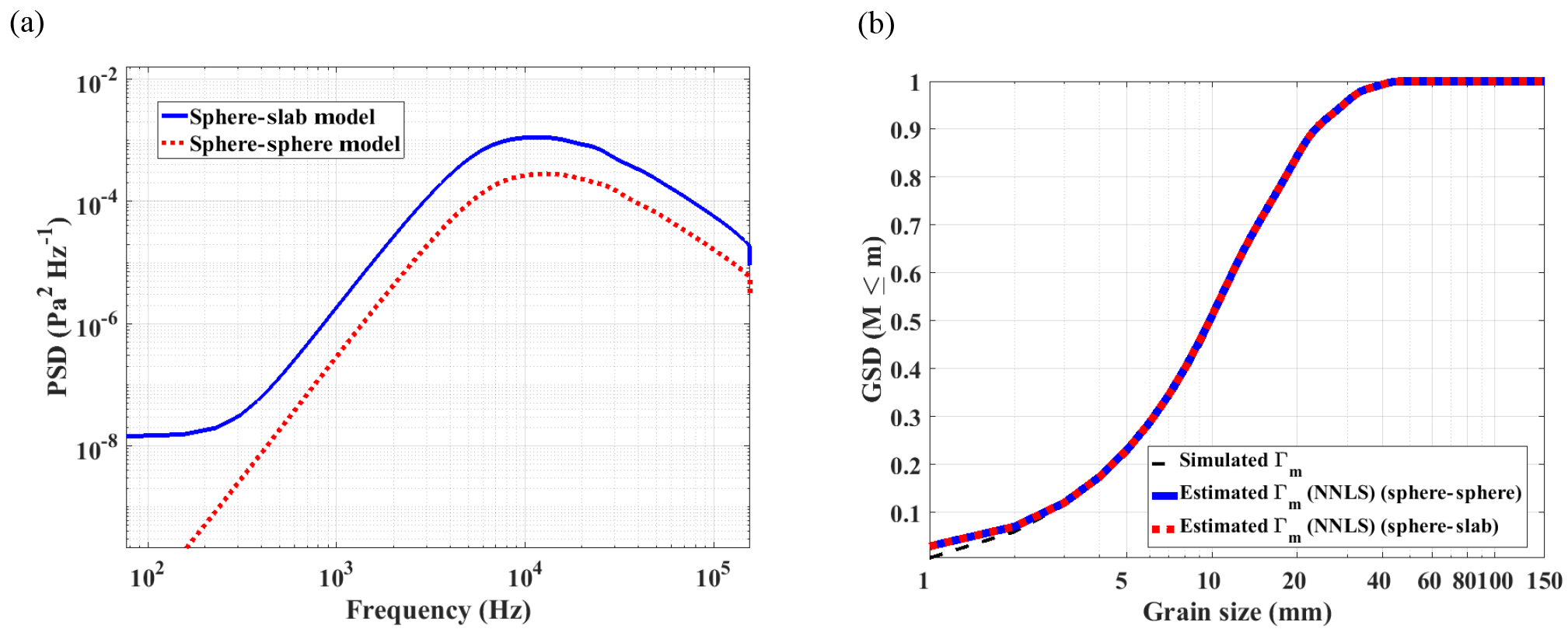
Figure 10(a) Modeled spectra using a log-normal GSD, , where D84=2 D50, D50=10 mm (see medallion); typical input parameters are given in Table 1 and Uimp=1 m s−1. Concerning the sphere–sphere impact, the impactor has the same size as the impactee; (b) inversion using the NNLS algorithm by acoustic spectra shown in (a).
This work deals with the development of a novel estimation strategy of bedload GSD from acoustic PSD. The spectrum inversion used the model based on sphere–slab impact, where the impacting sphere diameters range from K=1 mm to K=100 mm. The inversion of field experiments on the Isère River have shown in Fig. 10a interesting results in conformity with the assumptions enounced in Sect. 2.4.
The inversion considered four values of impact velocity m s−1. The best fit to the measured GSD by the TR sampler is when the impact velocity Uimp is between 0.01 and 0.1 m s−1, which could be possible for a large gravel bedded river like the Isère. To verify this, the apparent velocity of the bed material (see Rennie and Miller, 2004, for a definition) was measured by an aDcp at the moment of hydrophone experiments. This estimated value was at a maximum around 0.01–0.02 m s−1, which can be in accordance with the impact velocity modeling the best NNLS estimates.
The cross-sectional variation of the estimated D16, D50 and D84 by the NNLS algorithm follows the same trend of increasing values from the left to right banks as the bedload D50 measured by the TR sampler (Fig. 9b). However, the cross-sectional variability of sampled diameters is higher than the estimated one. This is explained by the fact that the hydrophone has the spatial integrative characteristic (Geay et al., 2017b). The phenomenon of signal integration is typical for rivers like the Isère, where high fluxes of bedload transport are concentrated only in a small portion across the section, i.e., in its center. In this case spatial homogeneity as stated in Sect. 2.4 is no longer valid. However, the powerful acoustic source makes noise all over the cross section, causing the sound sources to appear ubiquitous. This may be the reason that the inversion of acoustic PSD measured in the center (X=34 m), for Uimp=0.1 m s−1, still shows a good match to the sampling measurements in that position, only because of the high powerful acoustic source localized in this position.
Despite the consistent variation of the GSD across the river bed, measured by the sampler, the acoustic spectrum shapes shown in Fig. 6b are relatively stable, in the interval to Pa Hz−1. This suggests that measurements by hydrophone installed from one of the banks are not dramatically different from measurements by free floating hydrophones along the watercourse.
The propagation of sound throughout the local reach also raises some concerns about the quality of measured acoustic spectra. The proposed model Eq. (6b) has been elaborated by assuming a simple geometrical spreading model of the acoustic waves in the river. Bedload SGN spectra monitored by a hydrophone are not only dependent on bedload sizes, but are also affected by propagation effects. For example, an alpine river has been modeled as a Pekeris waveguide (Geay et al., 2017b). Consequently, it has been shown that the monitored spectra were slightly dependent on the hydrophone position in the lower frequency band. Another propagation effect concerns the frequency cutoff phenomena, due to acoustic propagation in waveguides (Geay, 2013; Geay et al., 2017b; Jensen et al., 2011; Rigby et al., 2016). In our case, the Isère River has enough large depth that the bandwidth of bedload is not being impacted. The pebble-sized particles that are up to 64 mm give SGN of dominating frequencies well above 1000 Hz, whereas the channel's depth of 2.5 m fixes the cutoff frequency to about 148 Hz, assuming a perfectly rigid bottom. Therefore, the bandwidth of bedload is far superior to the frequency cutoff in the Isère River, so there are no risks of inversion. However, SGN monitoring and the inversion technique for GSD determination are particularly adapted to large rivers. Generally, propagation effects are frequency-dependent and higher frequency ranges are more affected by attenuation or scattering effects. A solution to the nonlinear effects of acoustic propagation would be to determine the river's transfer function by active acoustic experiments (Rigby et al., 2016) and to construct laws of attenuation that will compensate for the loss (Wren et al., 2015).
At first sight, our comparison with Thorne (1985, 1986b)'s regression laws would be very naïve due to the nature of theories: we considered the sphere–slab impact, whereas the regression laws are from sphere–sphere impact phenomena. Therefore, the inversion is put into discussion when the river bed is no longer armored, and so, the model of impact between sphere and slab is debatable. Here, we target the large gravel rivers. The dictionaries Δ for both impact models use an impact velocity Uimp=1 m s−1, the material is granite and a GSD is simulated according to Recking's procedure (Recking, 2013), where D84=2 D50. When comparing the shapes of both simulated PSDs, shown in Fig. 10a, their respective frequency peaks fpeak are nearly identical. Likewise, the slopes of the spectra are found to be quite similar. Fig. 10b shows that the two solutions show no difference, except for a little disparity in the region of small grains. This proves that sphere–slab framework modeling of the collision between sediments and the river bed could work not only for stable conditions, but also for hydraulic events.
Another strong assumption used in modeling the PSD model of mixed impacts is that the particles are of spherical shapes. It is intuitively reasoned that the particle sphericity, shape factor and roundness also affect the acoustics of impacts. There are multiple possible ways of reckoning the equivalent diameter of a non-spherical particle. The particle's radius may be computed with respect to the curvature of the region of contact (see Chadwick et al., 2012; Goldsmith, 2003), with respect to the particle's mass centroid (Thorne, 1986b), which is in fact the a axis of the particle, or with respect to the b axis of the particle (Wyss et al., 2016b). Laboratory tests were conducted at the GIPSA laboratory, during which two pebbles of a size in the range 32–46 mm were impacted in a water pool along the three ellipsoid axes a, b, and c. The methodology of measuring the ellipsoid axes is found in Bunte and Abt (2001). It was found that the measured centroid frequencies take values from 3000 to 8000 Hz. If the regression law Eq. (9) is used, then the estimated diameters span the range from 23 to 73 mm, which is the repartition of all possible radii of curvature of the respective zones of contact. If the mode of sediment transport by sliding is the most frequent, then the particle c axis could be used to infer an equivalent diameter. If the rolling mode is more frequent, then the b axis would be more appropriate to work with. Finally, if the saltation is concerned, which makes the point of this work, then axes a and b are equally probable to be taken into account in modeling impacts.
A new strategy has been presented for data processing on hydrophone measurements for monitoring the bedload GSD in a gravel river bed. This strategy defines a forward model and a spectrum inversion approach. Firstly, the forward model combines generated spectra from collisions between a sphere and a slab. Secondly, the inversion procedure treats the forward model as a linear system of equations and uses algebraic methods of solving least square problems to obtain the GSD.
The forward model is based on a weighted sum of analytical energy spectral densities modeling the physics impact between a sphere and a slab. The weighting coefficients of the model represent a probability mass function which gives in the end the grain size distribution of bedload particles. The global sensitivity analysis of the PSD model of mixed impacts determined that the shape of the GSD has the biggest influence on the shape of the acoustic spectrum computed by Eq. (6b). Other important parameters are the median diameter and the impact velocity. However, the influences are from mixed interactions of parameters, and it is very hard, if not impossible, to obtain a complete analysis of the sensitivity of the analytical model of Eq. (6b).
The PSD model of mixed impacts works under the following strong assumptions: (1) the GSD is distributed everywhere in space and, in the same way, (2) the acoustic propagation is not frequency-dependent and, so, the spectrum shape is not affected by propagation in the river, (3) the impact velocity is invariant with the grain size, and (4) the impacting particles are of a spherical shape. The in situ experimentations showed that the integrative sound from all over the reach could render the first assumption verified (or true). In the case of the Isère River, the concentration of high transport rates in the middle of the cross section permits reliable measurements of bedload GSD by hydrophone from river banks.
The inversion method is a non-negative least square algorithm and it eliminates the negative solutions caused by ill-conditioned matrices. Concerning the least square approach for inversion, it is robust to noise.
The inversion of spectra from field trials on the Isère River proved that the method is highly reliable with no consideration of a priori information on bedform morphology of hydrological conditions. Surrogate methods for sediment transport in rivers were conceived with the idea of having access to information all over the reach and real time. In contrast to geophones and the Japanese pipe, the hydrophone technique does not require particular efforts to be installed in the watercourse.
The authors provide the Matlab codes reproducing the results presented in Figs. 2, 4, and 10 and Table 2. The codes are found at the following URL: https://drive.google.com/open?id=1-eiM49Q8PW4q3acX67wlMO-NQPFXnkwi.
If experimental data from Figs. 6, 7, and 9 are needed, please contact the authors.
| length of sediment (ellipses) axis | mm | |
| A | Hertzian acceleration | m s−2 |
| c | sound celerity in water | m s−1 |
| Δ | modeled dictionary of individual energy spectra | |
| Ei | Energy spectral density of the impact of the size class i, Eq. (7) | |
| Ei,x | energy of collision in a narrow frequency bandwidth x | Pa2 s Hz−1 |
| Elong | elastic modulus (Young's modulus) of rigid body | Pa |
| ESD | Energy spectral density | Pa2 s Hz−1 |
| D | generic notation for the grain diameter | mm |
| Deq | equivalent diameter (with respect to the grain's mass center) | mm |
| Di | grain size for i from 1 to K | mm |
| DTR | grain size class measured by Toutle River TR sampler | mm |
| D16, D50, D84 | the 16th, 50th and 84th percentiles of the grain size distribution | mm |
| f | linear frequency | Hz |
| fcentr | centroid frequency | Hz |
| fpeak | peak frequency | Hz |
| FAST | Fourier amplitude sensitivity test | |
| FT | Fourier transform | |
| Fs | Sampling frequency | Hz |
| F | Fourier transform operator | |
| Fimp | linear complex magnitude spectrum of the elastic impact, Eq. (5) | Pa |
| energy spectral density of the elastic impact, Eq. (6) | Pa2 s Hz−1 | |
| GSA | Global sensitivity analysis | |
| GSD | Grain size distribution | |
| γ | solution of the inversion written as a probability mass function | |
| γm | solution of the inversion written as a probability mass function, computed from the mass histogram of sediments (Eq. 10) | |
| Γ | solution of inversion (GSD) in the cumulative form | |
| Γm | solution of inversion (GSD) in the cumulative form, computed from (Eq. 11) |
| I | Histogram of rate of impacts | |
| Ii | Rate of impact of the size class i | no. imp s−1 |
| j | imaginary unit | |
| K | number of grain sizes classes | |
| LS | Least square problem | |
| ν | Poisson's ratio of rigid body | |
| NFFT | number of points for FT computation | |
| NNLS | Non-negative least squares | |
| ω | Angular frequency | rad s−1 |
| P | Power spectrum density of the noise from an elastic impact, Eq. (9a–b) | Pa2 Hz−1 |
| PMF | Probability mass function | |
| PSD | Power spectral density | Pa2 Hz−1 |
| r | reference measurement distance between the sensor and the center of the impact (see Fig. 1a and b) | m |
| ρs | density of sediment | kg m−3 |
| ρ | density of water | kg m−3 |
| SGN | Self-generated noise (noise generated by the transported sediments in collision) | |
| Si | sensitivity indices from the first-order global sensitivity analysis | |
| σ | the SD of a normal distribution (used in sensitivity analysis) | |
| Td | phase shift between the signals from the two objects in collision | s |
| t | time | s |
| τ | delayed time | s |
| t′ | time variable used in the convolution Eq. (1) | s |
| θ | angle of directivity acoustic sources – sensor | ∘ |
| Tc | duration of Hertzian contact | s |
| Td | delayed time (delayed propagation due to the geometry of particles) | s |
| Uimp | impact velocity | m s−1 |
| X | position on the cross section of the Isère River (marked on the bridge from the left to right banks) | m |
Table B1Coefficients C1…6 used in the analytical model of impact of Akay and Hodgson (1978).
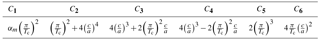
The acoustic pressure field generated by the Hertzian impact between sphere and slab is used to model elementary spectra contained in the dictionary Δ. The analytical temporal solutions, obtained from the integral convolution of Eq. (1) and using the geometric setup of Fig. 1b, are rewritten below from Akay and Hodgson (1978)'s paper. Thus, equations 6a-b and 7 from the paper of Akay and Hodgson (1978) are reformulated here in Eqs. (B1)–(B2) and, respectively, (B3). This analytical solutions model is a two-branch function, depending on the duration contact Td. Thereafter, the total acoustic pressure field, during and after the impact, is obtained by subtracting the individual pressure fields. Such a resulting waveform was shown in Fig. 2a and was modeled using Eq. (B3). It is important to note that another way to compute the energy spectral density of the impact is to numerically compute the Fourier transform on this equation.
where i=1 (the impacting sphere) or 2 (the mirrored sphere), both with the same radius a, is the delayed time, D is the sphere's diameter, c is the the velocity of speed, r is the reference distance, θ is the angle between source and sensor (see Fig. 1b) and the constants C1…6 are
The authors declare that they have no conflict of interest.
The study was supported by funding of doctoral studies from the Auvergne-Rhône-Alpes region through the “Communautés de Recherche Académique” (ARC no. 3) program for TP, by funding of a
research grant for TG from convention no. C43R5T5030 between
Électricité de France (EDF) and the Grenoble Institute of Technology,
and of research grant CHORUS
for Cédric Gervaise.
Edited by: Laurent Pfister
Reviewed by: two anonymous referees
Akay, A. and Hodgson, T. H.: Acoustic radiation fropm the elastic impact of a sphere with a slab, Appl. Acoust., 11, 285–304, 1978.
Barrière, J., Krein, A., Oth, A., and Schenkluhn, R.: An advanced signal processing technique for deriving grain size information of bedload transport from impact plate vibration measurements, Earth Surf. Proc. Land., 40, 913–924, https://doi.org/10.1002/esp.3693, 2015.
Barton, J. S.: Passive Acoustic Monitoring of Coarse Bedload in Mountain Streams, The Pennsylvania State University, College State, USA,, 2006.
Bedeus, K. and Ivicsis, L.: Observation of the noise of bed load, Int. Assoc. Hydrol. Sci., 19–31, 1963.
Belleudy, P., Valette, A., and Graff, B.: Passive hydrophone monitoring of bedload in river beds: first trials of signal spectral analyses, USGS, Scientific Investigations Report, 5091, 67–84, Virginia, USA, 2010.
Bogen, J. I. M. and Møen, K.: Bed load measurements with a new passive ultrasonic sensor, Erosion and Sediment Transport Measurement: Technological and Methodological Advances, International Association of Hydrological Sciences, Oslo, 19–21, 2001.
Bunte, K. and Abt, S.: Sampling Surface and Subsurface Particle-Size Distributions in Wadable Gravel- and Cobble-Bed Streams for Analyses in Sediment Transport, Hydraulics, and Streambed Monitoring, Gen. Tech. Rep. RMRS-GTR-74., Forest Service, Rocky Mountain Research Station, Fort Collins, Colorado, U.S. Department of Agriculture, 2001.
Bunte, K., Swingle, K. W., and Abt, S. R.: Necessity and Difficulties of Field Calibrating Signals from Surrogate Techniques in Gravel-Bed Streams: Possibilities for Bedload Trap Samplers, US Geol. Surv. Sci. Investig. Rep. 2010-5091, Bedload-Surrogate Monitoring Technologies, US Geol. Surv. Sci. Invest. Rep, 5091, 107–129, Virginia, USA, 2010.
Cannavó, F.: Sensitivity analysis for volcanic source modeling quality assessment and model selection, Comput. Geosci., 44, 52–59, https://doi.org/10.1016/j.cageo.2012.03.008, 2012.
Chadwick, J. N., Zheng, C., and James, D. L.: Precomputed acceleration noise for improved rigid-body sound, ACM T. Graphic., 31, 1–9, https://doi.org/10.1145/2185520.2335454, 2012.
Cukier, R. I., Fortuin, C. M., Shuler, K. E., Petschek, A. G., and Schaibly, J. H.: A Study of the Sensitivity of Coupled Reaction Systems to Uncertainties in Rate Coefficients. I. Theory, J. Chem. Phys., 59, 3873–3878, 1973.
Dell'Agnese, A., Mao, L., and Comiti, F.: Calibration of an acoustic pipe sensor through bedload traps in a glacierized basin, Catena, 121, 222–231, https://doi.org/10.1016/j.catena.2014.05.021, 2014.
Einstein, H. A.: The bed-load function for sediment transportation in open channel flows, Soil Conserv. Serv., 1026, 1–31, 1950.
European Commission: European Common Implementation Strategy for the Water Framework Directive (2000/60/EC), Water Directors under Swedish Presidency, Directive, 428, May, 2001.
Geay, T.: Mesure acoustique passive du transport par charriage dans les rivières [Passive Acoustic measurement of bedload transport in rivers], Université Joseph Fourier, Grenoble, 2013.
Geay, T., Belleudy, P., Gervaise, C., Habersack, H., Aigner, J., Kreisler, A., Seitz, H., and Laronne, J.: Passive acoustic monitoring of bedload in large gravel bed rivers, J. Geophys. Res.-Earth, 122, 528–545, https://doi.org/10.1002/2016JF004112, 2017a.
Geay, T., Belleudy, P., Laronne, J. B., Camenen, B., Gervaise, C., and Development, E.: Spectral variations of underwater river sounds 1, Earth Surf. Proc. Land., 42, 2447–2456, https://doi.org/10.1002/esp.4208, 2017b.
Gimbert, F., Tsai, V. C., and Lamb, M. P.: A physical model for seismic noise generation by turbulent flow in rivers, J. Geophys. Res. Earth, 119, 2209–2238, https://doi.org/10.1002/2014JF003201, 2014.
Goldsmith, W.: Impact, Dover Publications, Inc., Mineola, NY, USA, 2003.
Gray, J. R., Laronne, J. B., and Marr, J. D. G.: Bedload-surrogate monitoring technologies, US Geol. Surv. Sci. Investig. Rep., 5091, 1–37, available at: https://pubs.usgs.gov/sir/2010/5091/ (last access: 10 January 2013), 2010.
Heimann, F. U. M., Rickenmann, D., Turowski, J. M., and Kirchner, J. W.: sedFlow – a tool for simulating fractional bedload transport and longitudinal profile evolution in mountain streams, Earth Surf. Dynam., 3, 15–34, https://doi.org/10.5194/esurf-3-15-2015, 2015.
Hertz, H.: Über die Berührung fester elastischer Körper (On the vibration of solid elastic bodies), J. Reine Angew. Math., 92, 156–171, 1882.
Hubbell, D. W.: Apparatus and Techniques for Measuring Bedload, US Geol. Surv. Water-Supply Pap., US Govt. Print. Off., Washington, USA, 1748, 74, 1964.
Hunter, S. C.: Energy absorbed by elastic waves during impacts, J. Mech. Phys. Solids, 5, 162–171, 1957.
Jensen, F. B., Kuperman, W. A., Porter, M. B., and Schmidt, H.: Computational Oceanic Acoustics, Springer-Verlag, New York, 2011.
Johnson, P. and Muir, T. C.: Acoustic detection of sediment movement, J. Hydraul. Res., 7, 519–540, https://doi.org/10.1080/00221686909500283, 1969.
Jonys, C. K.: Acoustic measurement of sediment transport, Sci. Ser., 66, 1–64, 1976.
Kirchhoff, G. R.: Vorlesungen uber Matematische Physik”, Vol. 1, “Mechanik”, Dritte Auflage, Druck und Verlag von G. B. Teubner, Leipzig, 1, 316–320, 1883.
Koss, L. L. and Alfredson, R. J.: Transient sound radiated by spheres undergoing an elastic collision, J. Sound Vib., 27, 59–75, https://doi.org/10.1016/0022-460X(73)90035-7, 1973.
Krein, A., Klinck, H., Eiden, M., Symader, W., Bierl, R., Hoffmann, L., and Pfister, L.: Investigating the transport dynamics and the properties of bedload material with a hydro-acoustic measuring system, Earth Surf. Proc. Land, 33, 152–163, https://doi.org/10.1002/esp.1576, 2008.
Krein, A., Schenkluhn, R., Kurtenbach, A., Bierl, R., and Barrière, J.: Listen to the sound of moving sediment in a small gravel-bed river, Int. J. Sediment Res., 31, 271–278, https://doi.org/10.1016/j.ijsrc.2016.04.003, 2014.
Kuhnle, R. A.: Fluvial transport of sand and gravel mixtures with bimodal size distributions, Sediment. Geol., 85, 17–24, https://doi.org/10.1016/0037-0738(93)90072-D, 1993.
Lawson, C. L. and Hanson, R. J.: Solving Least-Squares Problems, Englewood Cliffs, NJ: Prentice Hall, 23, 161 pp., 1974.
Mao, L., Carrillo, R., Escauriaza, C., and Iroume, A.: Flume and field-based calibration of surrogate sensors for monitoring bedload transport, Geomorphology, 253, 10–21, https://doi.org/10.1016/j.geomorph.2015.10.002, 2016.
Mizuyama, T., Oda, A., Laronne, J. B., Nonaka, M., and Matsuoka, M.: Laboratory tests of a japanese pipe geophone for continuous acoustic monitoring of coarse bedload, Bedload-Surrogate Monit. Technol., USGS, Scientific Investigations Report, 5091, 319–335, 2010.
Muste, M., Baranya, S., Tsubaki, R., Kim, D., Ho, H., Tsai, H., and Law, D.: Acoustic mapping velocimetry, Water Resour. Res., 52, 4132–4150, https://doi.org/10.1002/2015WR018354, 2016.
Oppenheim, A. V and Verghese, G. C.: Signals, Systems and Inference – Class notes for 6.011: Introduction to Communication, Control and Signal Processing Spring 2010, Cl. notes 6.011 Introd. to Commun. Control Signal Process. – Massachusetts Inst. Technol., available at: http://scholar.google.com/scholar?hl=en&btnG=Search&q=intitle:Signals,+systems+and+inference#8, 2010.
Papanicolaou, A. N. (Thanos), Elkaheem, M., and Knapp, D.: Evaluation of a gravel transport sensor for bed load measurements in natural flows, Int. J. Sediment Res., 24, 1–15, https://doi.org/10.1016/S1001-6279(09)60012-3, 2009.
Parker, G.: Surface-based bedload transport relation for gravel rivers, J. Hydraul. Res., 28, 417–436, https://doi.org/10.1080/00221689009499058, 1990.
Parker, G.: Chapter 3: Transport of gravel and sediment mixtures, ASCE, 54, 1–162, 2002.
Recking, A.: An analysis of nonlinearity effects on bed load transport prediction, J. Geophys. Res.-Earth, 118, 1264–1281, https://doi.org/10.1002/jgrf.20090, 2013.
Recking, A.: A generalized thresholdmodel for computing bed load grain size distribution, Water Resour. Res., 52, 1–15, https://doi.org/10.1029/2008WR006912, 2016.
Rennie, C. D. and Millar, R. G.: Measurement of the spatial distribution of fluvial bedload transport velocity in both sand and gravel, Earth Surf. Proc. Land., 29, 1173–1193, https://doi.org/10.1002/esp.1074, 2004.
Rickenmann, D., Turowski, J. M., Fritschi, B., Wyss, C., Laronne, J., Barzilai, R., Reid, I., Kreisler, A., Aigner, J., Seitz, H., and Habersack, H.: Bedload transport measurements with impact plate geophones: comparison of sensor calibration in different gravel-bed streams, Earth Surf. Proc. Land., 39, 928–942, https://doi.org/10.1002/esp.3499, 2014.
Rigby, J. R., Wren, D., and Murray, N.: Acoustic Signal Propagation and Measurement in Natural Stream Channels for Application to Surrogate Bed Load Measurements, Halfmoon Creek, Colorado, 1566–1570, 2016.
Roth, D. L., Brodsky, E. E., Finnegan, N. J., Rickenmann, D., Turowski, J. M., and Badoux, A.: Bed load sediment transport inferred from seismic signals near a river, J. Geophys. Res.-Earth, 121, 725–747, https://doi.org/10.1002/2015JF003782, 2016.
Sobol, I. M.: Global sensitivity indices for nonlinear mathematical models and their Monte Carlo estimates, Math. Comput. Simulat., 55, 271–280, https://doi.org/10.1016/S0378-4754(00)00270-6, 2001.
Strang, G.: Linear Algebra and Its Applications, Thomson Brooks-Cole Publishing, Pacific Grove CA, USA, 487 pp., 2006.
Thorne, P. D.: The measurement of acoustic noise generated by moving artificial sediments, J. Acoust. Soc. Am., 78, 1013–1023, 1985.
Thorne, P. D.: An intercomparison between visual and acoustic detection of seabed gravel movement, Mar. Geol., 72, 11–31, https://doi.org/10.1016/0025-3227(86)90096-4, 1986a.
Thorne, P. D.: Laboratory and marine measurements on the acoustic detection of sediment transport, J. Acoust. Soc. Am., 80, 899–910, https://doi.org/10.1121/1.393913, 1986b.
Thorne, P. D.: An overview of underwater sound generated by interparticle collisions and its application to the measurements of coarse sediment bedload transport, Earth Surf. Dynam., 2, 531–543, https://doi.org/10.5194/esurf-2-531-2014, 2014.
Thorne, P. D. and Foden, D.: Generation of underwater sound by colliding spheres, J. Acoust. Soc. Am., 84, 2144–2152, https://doi.org/10.1121/1.397060, 1988.
Tsai, V. C., Minchew, B., Lamb, M. P., and Ampuero, J.-P.: A physical model for seismic noise generation from sediment transport in rivers, Geophys. Res. Lett., 39, https://doi.org/10.1029/2011GL050255, 2012.
Turowski, J. M., Badoux, A., and Rickenmann, D.: Start and end of bedload transport in gravel-bed streams, Geophys. Res. Lett., 38, 1–5, https://doi.org/10.1029/2010GL046558, 2011.
Wilcock, P. R. and Kenworthy, S. T.: A two-fraction model for the transport of sand/gravel mixtures, Water Resour. Res., 38, 1–12, https://doi.org/10.1029/2001WR000684, 2002.
Wilcock, P. R. and McArdell, B. W.: Surface-based fractional transport rates: mobilization thresholds and partial transport of a sand-gravel sediment, Water Resour. Res., 29, 1297–1312, 1993.
Wilcock, P., Pitlick, J., and Cui, Y.: Sediment Transport Primer: Estimating Bed-Material Transport in Gravel-Bed Rivers, Rocky Mountain Research Station, USDA Forest Service, RMRS-GTR-226, 2009.
Wren, D. G., Goodwiller, B. T., Rigby, J. R., Carpenter, W. O., Kuhnle, R. A., and Chambers, J. P.: Sediment-Generated Noise (SGN): laboratory determination of measurement volume, Proc. 3rd Jt. Fed. Interag. Conf., 10th Fed. Interag. Sediment. Conf. 5th Fed. Interag. Hydrol. Model. Conf. 19–23 Apr 2015, Reno, Nevada, D, 408–413, 2015.
Wyss, C. R., Rickenamnn, D., Fritschi, B., Turowski, J. M., Weitbrecht, V., and Boes, R. M.: Laboratory flume experiments with the Swiss plate geophone bed loadmonitoring system: 1. Impulse counts and particle size identification, Water Resour. Res., 52, 5216–5234, https://doi.org/10.1002/2014WR015716, 2016a.
Wyss, C. R., Rickenmann, D., Fritschi, B., Turowski, J. M., Weitbrecht, V., and Boes, R. M.: Measuring bed load transport rates by grain-size fraction using the swiss plate geophone signal at the Erlenbach, J. Hydraul. Eng., 142, 4016003, https://doi.org/10.1061/(ASCE)HY.1943-7900.0001090, 2016b.