Principal components of thermal regimes in mountain river networks

Description of thermal regimes in flowing waters is key to understanding physical processes, enhancing predictive abilities, and improving bioassessments. Spatially and temporally sparse data sets, especially in logistically challenging mountain environments, have limited studies on thermal regimes, but inexpensive sensors coupled with crowd-sourced data collection efforts provide efficient means of developing large data sets for robust analyses. Here, thermal regimes are assessed using annual monitoring records compiled from several natural resource agencies in the northwestern United States that spanned a 5-year period (2011–2015) at 226 sites across several contiguous montane river networks. Regimes were summarized with 28 metrics and principal component analysis (PCA) was used to determine those metrics which best explained thermal variation on a reduced set of orthogonal axes. Four principal components (PC) accounted for 93.4 % of the variation in the temperature metrics, with the first PC (49 % of variance) associated with metrics that represented magnitude and variability and the second PC (29 % of variance) associated with metrics representing the length and intensity of the winter season. Another variant of PCA, T-mode analysis, was applied to daily temperature values and revealed two distinct phases of spatial variability – a homogeneous phase during winter when daily temperatures at all sites were <3 ^∘C and a heterogeneous phase throughout the year's remainder when variation among sites was more pronounced. Phase transitions occurred in March and November, and coincided with the abatement and onset of subzero air temperatures across the study area. S-mode PCA was conducted on the same matrix of daily temperature values after transposition and indicated that two PCs accounted for 98 % of the temporal variation among sites. The first S-mode PC was responsible for 96.7 % of that variance and correlated with air temperature variation (r=0.92), whereas the second PC accounted for 1.3 % of residual variance and was correlated with discharge (r=0.84). Thermal regimes in these mountain river networks were relatively simple and responded coherently to external forcing factors, so sparse monitoring arrays and small sets of summary metrics may be adequate for their description. PCA provided a computationally efficient means of extracting key information elements from the temperature data set used here and could be applied broadly to facilitate comparisons among more diverse stream types and develop classification schemes for thermal regimes.

1 Introduction

Temperatures of flowing waters control many physicochemical processes (Likens and Likens, 1977; Gordon et al., 1991; Ducharne, 2008) and affect the ecology of aquatic organisms and communities (Isaak et al., 2017b; Neuheimer and Taggart, 2007; Woodward et al., 2010). Knowledge of thermal regimes, characterized as the annual sequence of temperature conditions specific to locations within river networks (Caissie, 2006), is key to understanding natural conditions and diagnosing anthropogenic impairments. Seminal work by Poff and colleagues (Poff and Ward, 1989; Poff et al., 1997) created a robust framework for describing flow regimes based on metric descriptions of magnitude, frequency, timing, duration, and variability that are largely transferrable to thermal regimes (Poole et al., 2004; Olden and Naiman, 2010). Recent studies have contributed useful derivations of temperature metrics (Arismendi et al., 2013; Chu et al., 2010; Rivers-Moore et al., 2013; Steel et al., 2016) or classification schemes based on a small number of pre-selected metrics (Maheu et al., 2016), but the limited availability of annual temperature records (Orr et al., 2015; Isaak et al., 2018a) has slowed broad development and adoption of thermal regime concepts. Data inadequacies are often compounded for montane riverscapes that are difficult to sample (Brown and Hannah, 2008; Isaak et al., 2013), a shortfall that needs to be overcome given the importance of these areas as climate refugia for cold-water biodiversity (Brown et al., 2009; Isaak et al., 2016b; Quaglietta et al., 2018) and as the focus of costly regional conservation strategies (Roni et al., 2002; Rieman et al., 2015).

Despite existing limitations, the importance of temperature to stream biota is well recognized and inculcated to regulatory standards based on metrics used within threshold-based approaches (Poole et al., 2004; Todd et al., 2008). Most often, those metrics represent some aspect of conditions during warm summer months when temperature sensitive species or life stages are thought to be most vulnerable (Ice et al., 2004; McCullough, 2010), which contributes to the preponderance of short monitoring records spanning only these months (Isaak et al., 2017a). However, thermally mediated ecological processes occur throughout the year (Neuheimer and Taggart, 2007; Olden and Naiman, 2010), so adequate understanding requires broader characterization of thermal conditions from annual data sets. While that may bring additional complexity, most warm season metrics are strongly correlated and therefore redundant (Isaak and Hubert, 2001; Dunham et al., 2005; Steel et al., 2016). If redundancy is also the norm among a broader array of annual temperature metrics, then multivariate data reduction techniques might be useful for identifying a few key aspects of thermal regimes.

Supporting that idea, Rivers-Moore et al. (2013) used principal component analysis (PCA) to describe covariation among 39 temperature metrics calculated for 82 South African stream sites and found that two PCs accounted for 75 % of the total variation among metrics. Similarly in the field of hydrology, Olden and Poff (2003) examined 171 flow metrics calculated from 420 gage sites across the United States (U.S.) and found that two to four PCs accounted for 76 %–97 % of variation in the data set. In addition to metric-based PCA that is commonly used in the hydrological sciences, several other PCA variants are standard analytical tools in the field of climatology and may be relevant for characterizing the dynamics of thermal regimes (Richman, 1986; Demsar et al., 2013). Most notably, PCA can be done on repeated measurements of a single variable to identify common spatial or temporal behavior among monitoring stations. In the climatology literature, for example, empirical orthogonal function analysis (S-mode PCA in the taxonomy of Richman, 1986) is used to determine which sites covary temporally as a means of developing regionalization schemes for precipitation, air temperatures, or wind speeds (Piechota et al., 1997; Jiménez et al., 2008; Martins et al., 2012). If common temporal patterns are identified, it suggests potential redundancy in the monitoring network and the information can be used to refine future sampling designs. The closely allied T-mode PCA identifies dominant spatial patterns in data sets and the times when these phases occur (Richman, 1986; Gallacher et al., 2017). A single dominant spatial pattern suggests the spatial distribution of a variable is temporally consistent, whereas more than one spatial phase suggests change points and different states.

The advent of inexpensive sensors, combined with regulatory requirements and concerns about climate change, have led to the recent expansion in temperature monitoring networks for rivers and streams (Isaak et al., 2010; Rivers-Moore et al., 2013; Hilderbrand et al., 2014; Luce et al., 2014b; Trumbo et al., 2014; Hannah and Garner, 2015; Jackson et al., 2016; Molinero et al., 2016; Daigle et al., 2016; Mauger et al., 2016; Steel et al., 2016). What was once a data dearth is becoming a deluge and opportunities exist to study thermal regimes with robust data sets. Here, we use annual temperature records compiled from several natural resource agencies for 226 monitoring sites in a mountainous landscape to conduct an initial assessment of thermal regimes. We limit the geographic scope of our effort to several adjacent river basins in the northwestern U.S. that are geologically and topographically similar but which have particularly dense monitoring networks to maximize analytical flexibility. Our objectives were to (1) provide a basic description of the annual thermal characteristics in mountain rivers and streams because these are rare within the literature, (2) develop metrics to describe thermal regime characteristics based on magnitude, frequency, timing, duration, and variability, and (3) explore spatiotemporal variation among those metrics and temperature dynamics in relation to basin morphology and hydroclimatic conditions to better discern the principal components of thermal regimes and their regulating factors.

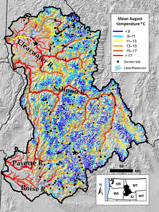
Figure 1 Locations of 226 monitoring sites overlaid on an August stream temperature scenario for the 29 600 km network in the study area. Stars denote where air temperature and stream discharge data were obtained from a low-elevation site (294 m, northern station) and a high-elevation site (1850 m, southern station).

Figure 2 Annual cycle of mean daily water temperatures (a), air temperatures (b), and discharge (c) at a high-elevation site and a low-elevation site during 2 contrasting climate years. Discharge values at the high-elevation site are multiplied by 10 for better visibility.

2 Study area

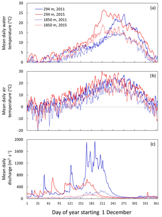
The study area encompasses 79 500 km² of mountainous, topographically complex terrain that spans a broad elevation range of 200–3600 m at a latitude of 45^∘ N in the northwestern United States (Fig. 1). Climate is characterized by cold, wet winters with moderate to heavy snow accumulations at high elevations and hot, dry summers. Hydrographs are typical of snowmelt runoff systems, with high flows during spring and early summer and low flows during late summer, fall, and winter (Fig. 2). Vegetation is dominated by conifer forests except at low elevations and south facing aspects where grasses and shrubs predominate. Wildfires are common within the landscape and burned 8 % of the area from 2011 to 2015 (Morgan et al., 2014). Parent geology consists mostly of resistant granites of the Idaho Batholith and a smaller easterly portion of intrusive volcanics (Bond and Wood, 1978; Meyer et al., 2001). Both geologies are heavily dissected and stream valleys are V-shaped except for some alpine valleys at the highest elevations that were once glaciated. Human population densities are low except along wider segments of river valleys where fertile floodplains and easy access to water accommodate small amounts of agriculture and ranching. Most of the study area is publicly owned (81 %) and federally administered by the United States National Forest Service and Bureau of Land Management for a variety of land-use, recreational, and conservation purposes. Unpaved road networks have been developed in some drainages for timber harvest, but many drainages are protected in large wilderness areas with minimal anthropogenic effects or roads (Swanson, 2015).

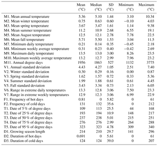
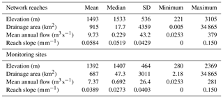
Table 1 Descriptive statistics for spatial attributes of the study network and 226 monitoring sites with annual temperature data in the northwestern United States.

River networks and temperature data set

Rivers and streams within the study area were delineated using the 1:100 000-scale National Hydrography Dataset (NHD; http://www.horizon-systems.com/NHDPlus/index.php, last access: 2 December 2018; McKay et al., 2012), which was attributed with mean annual flow values from data at the Western U.S. Stream Flow Metrics website (http://www.fs.fed.us/rm/boise/AWAE/projects/modeled_stream_flow_metrics.shtml, last access: 2 December 2018; Wenger et al., 2010). To highlight the perennial subset of the network where temperature monitoring occurred, reaches with annual flows less than 0.03 m³ s⁻¹ were removed from the network, as were reaches with channel slopes >15 %, and those coded as intermittent in the NHD (Fcode=46 003). Filtering reduced the original network extent from 58 000 to 29 600 km with streams flowing at elevations of 221–3105 m. To visualize thermal heterogeneity in the network, a scenario representing mean August temperatures for a baseline climate period of 1993–2011 was downloaded from the Northwestern Stream Temperature website (NorWeST: https://www.fs.fed.us/rm/boise/AWAE/projects/NorWeST.html, last access: 2 December 2018; Isaak et al., 2016a) and linked to the NHD reaches (Fig. 1). Several large rivers drain the area in a generally westerly direction, the largest of which is the Salmon River with a mean annual discharge of 315 m³ s⁻¹ and a basin that comprised 44 % of the study area. Six large dams and reservoirs are in downstream portions of the network (three in the Boise River basin, two in the Payette River basin, and one in the Clearwater River basin), but these affect thermal conditions in less than 300 km of river and no temperature data were used from these sections. Spatial attributes and environmental characteristics of the study area network are summarized in Table 1.

To obtain a water temperature data set for analysis, we intersected the filtered network with the NorWeST database of daily temperature summaries (Chandler et al., 2016) and extracted data for sites that had mean daily temperature values on at least 70 % of the days from 1 December 2010 to 30 November 2015. We started the thermal year on 1 December because temperatures usually reach their annual lows by this date and the 3-month period thereafter constituted a logical winter season (i.e., December, January, February). Subsequent 3-month periods were considered to be spring (March, April, May), summer (June, July, August), and fall (September, October, November) seasons. NorWeST temperature records were supplemented with additional data solicited from hydrologists and fisheries biologists employed by the Idaho Department of Fish and Game and the U.S. Forest Service, and we also downloaded data from online databases maintained by the Columbia Habitat Monitoring Program (https://www.champmonitoring.org/Home/Index, last access: 2 December 2018) and the NOAA Northwest Fisheries Science Center (https://www.webapps.nwfsc.noaa.gov/WaterQuality/, last access: 2 December 2018). Geographic gaps in monitoring were identified using geospatial analysis (e.g., Jackson et al., 2016) and additional sensors were strategically deployed where needed (Isaak et al., 2010, 2013). Data from the different sources were recorded at a variety of sub-daily intervals, so records were summarized to mean daily temperatures for standardization. Data were collected using different sensor models (TidbiT, Stowaway, and Pendant models from Onset Computer Corporation, Pocasset, Massachusetts, USA; Temp101a model from MadgeTech, Warner, New Hampshire, USA), which had measurement accuracies of ±0.2 to ±0.5 ^∘C and resolutions of 0.02 to 0.14 ^∘C based on manufacturer specifications and calibration tests we performed. Sensors were deployed using underwater epoxy or steel cables for connection to large boulders and other immobile channel structures and were shielded from direct sunlight (Isaak et al., 2013; Stamp et al., 2014). Temperature records were subject to standard quality assurance–quality control measures as described elsewhere (Chandler et al., 2016).

The stream temperature data set consisted of records from 226 sites across a range of elevations, stream sizes, and reach slopes (Fig. 1; Table 1). Although we set the minimum threshold for record completeness at 70 % during the 5-year period, the average completeness of records was higher at 88 %. Missing daily values were imputed using the MissMDA package (Missing Values with Multivariate Data Analysis; Josse and Husson, 2016) in R (R Development Core Team, 2014) because temporal covariation among proximate stream temperature sites is usually strong. That was confirmed in our data set by the high correlations between observed daily temperatures and predictions from the imputation technique, which ranged from r=0.98 to 0.99. All temperature records at the 226 sites were complete after imputation and consisted of 1826 mean daily temperatures from 1 December 2010 to 30 November 2015. Climatological variation during the same period was described using discharge data downloaded from the National Water Information System database (https://waterdata.usgs.gov/usa/nwis/nwis, last access: 2 December 2018) for a high-elevation gage site at 1850 m and a low-elevation gage site at 294 m and air temperature data from monitoring stations in the Cooperative Observer Network (https://www.ncdc.noaa.gov/data-access, last access: 2 December 2018) that were near the gage sites (Fig. 1).

Table 2 Temperature metrics used to describe thermal regimes of mountain rivers and streams.

Table 3 Descriptive statistics for temperature metrics used to describe thermal regimes at 226 monitoring sites in mountain river networks. Statistics were calculated from the imputed time series and mean daily values for the period 2011–2015.

3 Data analysis

3.1 PCA of thermal metrics

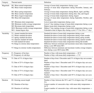
Prior to calculating metrics for thermal characteristics, mean daily temperatures for 365 days were calculated from the 5 years of data at each site to provide representative values. Twenty-eight temperature metrics were then calculated to describe aspects of those annual records based on five categories associated with magnitude, variability, frequency, timing, and duration (Tables 2 and 3). Metrics were similar to those used in previous studies of thermal regimes (Arismendi et al., 2013; Chu et al., 2010; Rivers-Moore et al., 2013; Steel et al., 2016) and in studies assessing the effects of peak summer temperatures on the distribution and abundance of aquatic organisms (Dunham et al., 2003; Huff et al., 2005; Isaak et al., 2017b). A wide range of variability occurred among sites where mean annual temperatures ranged from 3.1 to 10.3 ^∘C and annual standard deviations ranged from 2.51 to 7.40 ^∘C (Table 3). Relationships among the thermal metrics were described by conducting PCA on a data matrix in which columns represented the 28 metrics and rows were the 226 monitoring sites. Linear combinations of the data were estimated with coefficients equal to the eigenvectors of their correlation matrix, which were the principal components (PCs; Pearson, 1901; Sergeant et al., 2016). The first principal component accounted for the largest possible variance in the data set and succeeding components accounted for the largest portions of the remaining variance while being orthogonal (i.e., uncorrelated) to the preceding components. Correlations, or loadings, between each metric and the PCs were also calculated to assist in subsequent interpretations. The Princomp procedure in SAS (SAS Institute Inc., 2015) was used to conduct the PCA. To describe geographical relationships, PC scores were mapped to the 226 temperature sites and bivariate correlations were calculated with descriptors of network conditions such as elevation, reach slope, and discharge summarized in Table 1.

3.2 PCA of daily water temperatures

To assess the consistency of spatial temperature patterns among monitoring sites, a T-mode PCA (Richman, 1986) was done on a data matrix of mean daily temperatures in which the columns were the 365 days starting on 1 December and the rows were the 226 monitoring sites. In this analysis, the number of principal components explaining significant variation indicates the number of distinct spatial phases that occur throughout the year (Gallacher et al., 2017). Eigenvector loadings on the dominant PCs were plotted for each day of the year to describe when each phase occurred, and mean daily temperatures were mapped during these periods for visualization.

To assess temporal covariance among sites, an S-mode PCA (Richman, 1986) was done by transposing the T-mode data matrix so that monitoring sites were columns and the time-ordered daily mean temperatures were rows. Because hydroclimatic conditions among years could have affected the results, the S-mode PCA was done not only for the 5-year averages of daily water temperatures, but also on the disaggregated time series of 1826 daily values at the 226 monitoring sites. Concordance between the S-mode PC scores, air temperature, and discharge was examined post hoc by plotting standardized time series and calculating bivariate correlations.

Figure 3 Linear regression trends between elevation and mean monthly temperatures at 226 river and stream sites during 2013 (data values are not shown for clarity). Values next to the trend lines are regression slopes and r² values from the regressions.

4 Results

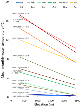
Water temperatures within the study area network exhibited spatial and temporal variation that reflected the local topography and annual hydroclimatic cycle. The annual temperature cycle is illustrated in Fig. 3 by the slopes of linear regressions between mean monthly temperatures and elevation at the 226 monitoring sites throughout the course of the year in 2013. No elevation trend occurred during cold winter months when many sites had water temperatures at or near 0 ^∘C and were frequently exposed to subzero air temperatures. As temperatures warmed during the spring a small elevation trend appeared, which became most pronounced (approximately $-\mathrm{0.37}{}^{\circ }\mathrm{C}/\mathrm{100}\mathrm{m}$) during peak temperatures in the months of July and August. Examples of inter-annual variation are shown in Fig. 2, which contrasts the extreme conditions observed in 2011 and 2015. The former year was relatively cool with a large winter snow accumulation and spring runoff, whereas 2015 had below average snowfall, low runoff, and particularly warm early summer air temperatures. As a result, the median discharge date occurred 1–2 months earlier in 2015 than in 2011 and peak water temperatures were 4–5 ^∘C warmer.

Table 4 Loadings of 28 temperature metrics on the first four principal components in a PCA of annual temperature records from mountain river networks in the northwestern United States.

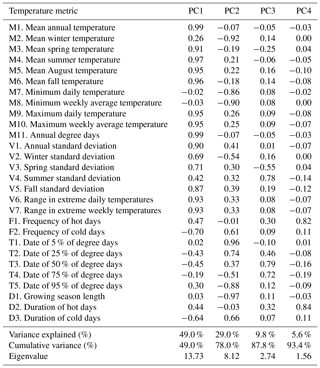
Table 5 Correlations among stream temperature principal components and spatial attributes of 226 monitoring sites with annual data from river networks in the northwestern United States.

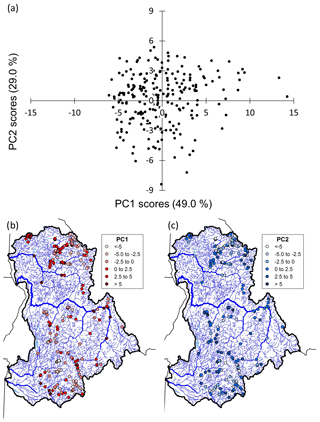
Figure 4 Ordination plot that shows principal component scores of the first two axes derived from water temperature data measured at 226 sites and summarized with 28 thermal metrics (a). (b) and (c) show principal component scores mapped to network locations.

Four PCs accounted for 93.4 % of the variation in the 28 temperature metrics (Table 4). The first PC explained 49 % of the variation and was strongly correlated with metrics that represented magnitude and variability during most seasonal periods. Correlations between PC1 scores and elevation ($r=-\mathrm{0.59}$) and mean flow (r=0.58) suggested gradients in these network characteristics were important controls on this component of thermal regimes (Table 5). PC2 explained 29 % of thermal variation and represented the length and intensity of the winter period, with strong loadings for mean winter temperature, minimum temperature, and timing metrics that determined growing season length. PC3 accounted for 9.8 % of total variation and was associated with summer temperature variability and two timing metrics, whereas PC4 accounted for 5.6 % of thermal variance. An ordination plot of scores from the two dominant PCs showed a symmetrical distribution except for several sites with large positive scores on the first axis that were from large rivers at low elevations and had the warmest temperatures (Fig. 4a). A map of PC1 scores indicated that the spatial pattern in magnitude and variability (Fig. 4b) was congruent with the network scenario of mean August temperatures as would be expected (Fig. 1). In fact, the correlation between PC1 scores and the NorWeST August scenario predictions at the 226 monitoring sites was strong at r=0.86. The PC2 map showed several clusters of stream sites with high scores scattered throughout the study area (Fig. 4c), which tended to be associated with lower reach slopes (Table 5).

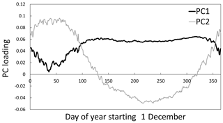
Figure 5 T-mode PCA results showing times when dominant spatial phases occurred in water temperatures at 226 sites based on principal component eigenvector loadings during an average year.

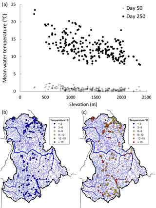
Figure 6 Thermal patterns during two periods with distinct spatial phases based on T-mode PCA results (a). Day 50 occurs in mid-January and represents the homogenous winter period (b), whereas day 250 occurs in late July and represents the heterogeneous period (c).

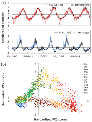
Figure 7 S-mode PCA results showing principal component scores that describe temporal patterns in mean daily water temperatures for 226 stream sites during 5 years (a). Average daily air temperatures and discharge values from two monitoring stations are aligned with the principal component scores for comparative purposes. A plot of PC1 versus PC2 reveals that variation along the two axes differs by monthly and seasonal periods (b).

In the T-mode analysis, the first two PCs explained 88 % of the total variation in mean daily temperatures. A plot of the daily eigenvector loadings indicated that one distinct spatial phase occurred in the winter and a second phase spanned the year's remainder (Fig. 5). Phase transitions occurred around days 100 and 350, which closely aligned with the abatement and onset of subzero air temperatures in the study area (Fig. 2). Figure 6 illustrates the spatial patterns characteristic of the two phases by mapping mean daily water temperatures at the monitoring sites on days 50 and 250, which occurred in mid-January and late July, respectively. Temperatures during the winter phase were spatially homogenous and exhibited a narrow range from 0 to 2.5 ^∘C, whereas the non-winter phase was heterogeneous and had a broader temperature range from 7.6 to 23.4 ^∘C.

In the S-mode analysis, the first PC accounted for 98 % of the variation when applied to the average year of 365 daily temperatures at the 226 monitoring sites. Nearly an identical result was obtained when the analysis was repeated on the disaggregated time series of 1826 daily temperatures, as PC1 then explained 96.7 % of total variation (Fig. 7a). The correlation between PC1 scores and mean daily air temperatures in the disaggregated series was strong (r=0.92), suggesting that water temperatures were responding coherently to variability in air temperatures across the study area. A second PC accounted for 1.3 % of water temperature variation in the disaggregated series and was strongly correlated with variation in mean daily discharge (r=0.84). A plot of PC1 versus PC2 indicated that variation along these axes corresponded to monthly and seasonal periods (Fig. 7b). As was expected, little variation occurred during the cold winter months, but during spring and early summer, variation was observed along both axes as air temperatures warmed and snowmelt runoff created a large discharge pulse. Once discharge returned to baseflow conditions in late summer, variability along PC1 was the primary signal until air temperatures cooled significantly in late fall and the homothermous period began.

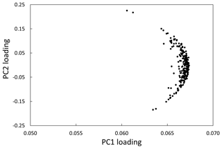
Figure 8 Plot of S-mode eigenvector loadings from 226 stream sites on PC1 and PC2. Note that the range of variation in the PC1 loadings is small relative to the loadings along PC2, which indicates that most of the differences among sites were associated with the second principal component.

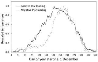
Figure 9 Annual water temperature timing patterns reconstructed from S-mode PCs using the mean eigenvector loading value for PC1 and ±0.16 for PC2 to demonstrate the effects of strong negative loadings and positive loadings on PC2.

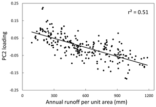
Figure 10 Relationship between the S-mode eigenvector loadings from PC2 and the annual unit-area runoff in basins upstream of 226 water temperature sites.

Although PC1 and PC2 are linearly uncorrelated, the loop structure of Fig. 7b indicates there was some mutual information and that one driver of temperature variation was out of phase with the other. Examining this more closely by plotting the site loading values on each component from the S-mode analysis, we see little variability among the loadings for PC1 relative to the much larger range of loading values for PC2 (Fig. 8). This confirms that PC1 represented the common behavior among all stream sites and that deviations in timing of water temperature increases and decreases were dictated by PC2. As a result, when annual temperature signals were reconstructed for two sites from the PCs based on the mean loading value for PC1 and ±0.16 for PC2 to represent strong negative and positive loadings, the expected timing shift was apparent (Fig. 9). Notably, the site with the −0.16 PC2 loading had a later, sharper rise in water temperature that peaked in late summer approximately 1 month after the site with the positive loading. The correspondence of PC2 to stream discharge in Fig. 7a suggests the timing shift could be related to runoff patterns. And indeed, the annual unit-area runoff for the basins associated with the 226 sites was a strong predictor of the PC2 loadings in a linear regression (r²=0.51; Fig. 10). Site elevation provides some indication of rainfall–snowfall fraction that may help explain timing shifts, but this covariate added little predictive capacity beyond annual runoff when examined across all sites (r²=0.54). However, when sites with basin sizes less than 50 km² were examined (because site elevation relates more strongly to mean basin elevation in smaller basins), elevation accounted for a large increase in the explainable variance of PC2 loadings beyond that attributable to annual runoff (r²=0.69). Although orographic enhancement of precipitation is evident in the study area, there is enough difference in circulation patterns across the north–south extent of the area that elevation and annual runoff were only weakly correlated in the small basins ($r=-\mathrm{0.2}$), so the elevation effect was largely independent of annual precipitation. As a result, both factors appeared to contribute to the PC2 loadings such that either wetter or colder locations had more negative loadings and later rises in water temperatures.

5 Discussion

5.1 Thermal regimes in mountain settings

Thermal regimes in the mountain river networks we studied were simple and responded relatively coherently to climatic variability across a geomorphically consistent area with few reservoirs. Strong seasonal patterns in water temperatures characteristic of temperate latitudes were apparent in response to the primary signal set by the annual air temperature cycle and accompanying changes in solar radiation. Not surprisingly given the pronounced elevational gradients in the study landscape, the dominant regime aspect represented by PC1 in the metric-based PCA was associated with magnitude. Less expected was that many of the variability metrics also loaded heavily on the first PC because variation has been treated as a distinct element of thermal regimes (e.g., Steel et al., 2012; Kovach et al., 2018). The concurrence of magnitude and variability metrics probably also relates to elevation and changes in the importance of groundwater buffering, which both cools streams and dampens diurnal and seasonal variations (Caissie and Luce, 2017). For example, the coldest streams at the highest elevations are usually strongly buffered by groundwater inputs derived from large annual snowpacks in mountain environments and often show limited thermal variability (Luce et al., 2014b; Isaak et al., 2016b). Downstream from the headwaters, the proportional inputs of groundwater decrease and streams are more coupled to climatic variability even as their average temperatures increase due to solar gains over longer flow distances (Caissie, 2006). In contrast to the metrics associated with PC1, metrics that described the winter period and the extent of the growing season largely defined PC2. This “winter” PC is probably common to stream thermal regimes in mountain landscapes where subzero air temperatures are frequent and result in prolonged periods with water temperatures near 0 ^∘C. The orthogonal nature of PC1 and PC2 suggests that streams with otherwise similar magnitude and variance structures will sometimes differ substantially with regards to their winter and growing seasons – a distinction that could have important implications for biological communities or stream physicochemical processes.

Our results also suggest that important local nuances in water temperature dynamics like the differences in timing of spring warming and peak temperatures may emerge from the interactions among annual climate cycles, basin geomorphology, and hydrology. Because precipitation, air temperatures, snowpack, runoff volume, and runoff timing are all evolving in response to climate change in mountain environments across the study region (Mote et al., 2005; Luce et al., 2013) and globally (Stewart, 2009), better understanding of these connections is needed. In particular, more insight into the relationship of water temperatures with annual unit-area runoff and whether the underlying mechanisms relate to changes in snowpack accumulation (Luce et al., 2014a; Lute and Luce, 2017), snowmelt timing and rate (Musselman et al., 2017), the volume of water stored in groundwater (e.g., Tague et al., 2007), or the outcomes of extreme low flows (e.g., Kormos et al., 2016; Luce and Holden, 2009) could lead to better predictions about water temperatures and the evolution of thermal regimes in response to expected changes in air temperatures and precipitation.

5.2 Implications for modeling and monitoring

Water temperature models are often developed for use in ecological assessments and to understand how habitat degradation or restoration efforts may affect thermal regimes (Benyahya et al., 2007; Gallice et al., 2015; Dugdale et al., 2017). Our results, like several previous studies that have compared multiple temperature metrics (Isaak and Hubert, 2001; Rivers-Moore et al., 2013; Steel et al., 2016), confirm that numerous metrics are strongly correlated and provide redundant information. The specific choice of a metric, therefore, may not be critical as long as it represents an important aspect of a thermal regime and is suited to the goals of a study. Metrics associated with temperature magnitude and variability, which have been the focus of most modeling efforts, are good choices because they represent significant portions of the information about thermal regimes and have been shown on many occasions to be important determinants of ecological attributes such as species distributions and abundance or physical processes in streams and rivers (Isaak et al., 2017b; Webb et al., 2008). Our preferred metrics in previous research have been mean August or mean summer temperatures because the data records for their calculation are typically available at the largest number of sites in mountain environments, which maximizes sample sizes and minimizes the distances over which interpolations are made when developing and applying network-scale temperature models (e.g., Detenbeck et al., 2016; Isaak et al., 2017a). Metrics based on longer-term means rather than short-term daily or weekly maxima are also more stable and easier to predict (Isaak et al., 2010; Turschwell et al., 2016), although a focus on the latter metrics is often mandated within regulatory environments and may negate these considerations (Todd et al., 2008; McCullough, 2010).

Comparatively little effort has gone towards modeling temperature metrics associated with growing season length or the dates of spring and winter season onset, despite the significant information these metrics provide about thermal regimes and their relevance to the phenology and life histories of organisms that constitute aquatic communities (Huryn and Wallace, 2000; Neuheimer and Taggart, 2007). These aspects of thermal regimes, as well as magnitude and variability characteristics, are also likely to be evolving in response to climate change, so new models are needed to provide forecasting abilities about changes later this century. Rather than focusing on individual metrics, researchers could also instead use PCA to efficiently summarize multiple temperature metrics and then model the eigenvector loadings that define one or more of the principal components. This approach would maximize the amount of thermal information represented by a response metric, but would yield results that were more ambiguous to interpret.

The growth of new stream and river temperature monitoring and data collection activities has been remarkable in recent years. Although optimization of those efforts ultimately depends on local considerations, some general guidelines emerge from this work that may be applicable to other areas. For example, the coherent behavior we observed among temperatures at many sites suggests that a limited number of monitoring stations will often be sufficient to represent the temporal dynamics of thermal regimes. Those stations would need to be spread geographically and along major environmental gradients and replicated to mitigate against sensor losses, but 20–30 stations might prove sufficient at scales comparable to our study area. Given low sensor costs and the availability of standardized data collection protocols (Isaak et al., 2013; Stamp et al., 2014), monitoring arrays could also be crowd-sourced effectively if site locations were coordinated and chosen strategically using geospatial analyses to describe and stratify networks for sample allocation (Jackson et al., 2016). Monitoring networks might also be supplemented by incorporating data from sites established for other purposes such as documenting thermal responses to habitat restoration efforts (Nichols and Ketcheson, 2013) or disturbances associated with land management, wildfires, or livestock grazing (Mahlum et al., 2011; Nusslé et al., 2015). In fact, those factors motivated collection of many of the data sets compiled for this analysis, although supplementation with additional sites was needed to ensure adequate coverage within the study area.

If one of the goals of temperature data collection efforts is to develop accurate prediction maps that show spatial variation in one or more thermal metrics (e.g., Isaak et al., 2017a; Steel et al., 2016), monitoring sites may need to be established more densely than the temporal considerations discussed above otherwise suggest. Spatial autocorrelation in temperature metric values is minimal in mountain river networks beyond distances of 10–100 km (Isaak et al., 2010; Zimmerman and Ver Hoef, 2017), so this level of sensor spacing would be required to generate the most accurate maps. Given the extent of many river networks, that could translate into a large number of sites, but most of these could be monitored for short periods while temporal dynamics were represented by a subset of long-term sites because temporal covariance among sites would be strong. Costs associated with numerous sensor deployments could be prohibitive, so aggregation of existing data sets from multiple natural resource agencies into a centralized database often becomes an attractive option. Moreover, if those central databases are made publicly accessible, professionals from the contributing agencies may begin to coordinate data collection activities more consistently and effectively across larger areas (e.g., Isaak et al., 2018b).

As new data collection and database development efforts proceed, it is commonly the case that temperature records have inconsistent period lengths or missing values. Usually it is desirable to have complete records for analysis, so missing values are sometime imputed based on the correlations between two monitoring site records that strongly covary (e.g., Rivers-Moore et al., 2013). However, the process can be tedious if required at more than a few sites, so an efficient improvement is offered by the imputation technique described by Josse and Husson (2012) that is easily used in the MissMDA software package (Josse and Husson, 2016) for the R statistical program (R Development Core Team, 2014). This technique examines and uses correlations among multiple site records simultaneously to estimate missing values by first applying standard PCA to the incomplete data set where missing values are replaced with the respective record mean. Data are then reconstructed from the PCs, and the initial analysis step is repeated but with missing values replaced using estimates from the reconstructed data. The process is repeated until convergence, and the missing values in the original data records are ultimately replaced with estimates from the last PCA reconstruction (Josse and Husson, 2012). Care should be taken against overreliance on the technique to impute particularly sparse records, but the MissMDA package provides a useful tool for addressing gaps when working with large temperature data sets or time series of other measurements common to hydrology such as gage discharge records (e.g., Isaak et al., 2018a).

6 Conclusions

Our analysis of thermal regimes follows previous work that has proven fundamental to advancing the understanding of hydrologic regimes (Poff et al., 1997; Olden and Poff, 2003) but also adds novel applications of PCA variants from the field of climatology that hold utility for stream temperature research and monitoring design. Insights from those applications indicate that thermal conditions in the mountain river networks studied here were strongly coherent through time, exhibited two distinct spatial phases, could be adequately described by a few principal components or allied metrics, and reflected landscape geomorphology and hydroclimatic conditions. A logical next step involves application of PCA techniques to larger stream and river temperature data sets at regional, continental, or intercontinental scales to encompass greater heterogeneity and discern the geographic domains over which distinct thermal regimes are operable. Across sufficiently diverse landscapes, we might expect to find classes of thermal regimes that, at a minimum, mimicked previously described classes of hydrologic regimes (e.g., rainfall, snowmelt, spring groundwater, and regulated), but possible divergences from, or additions to, these categories would be useful to ascertain. In a national-scale assessment for the United States, Maheu et al. (2016) classified stream thermal regimes into six categories, but the 135 temperature stations that supported the analysis were limited in comparison to a drainage network comprised of millions of kilometers. Subsequent iterations on that effort could document additional, undescribed thermal classes and might also prove beneficial by developing detailed maps of classification schemes to aid in assessments of ecological conditions or anthropogenic effects on stream thermal regimes. As research on the topic of thermal regimes matures, syntheses with flow regime concepts and databases could also be sought to more fully describe the hydroclimatic conditions of flowing waters.