the Creative Commons Attribution 4.0 License.
the Creative Commons Attribution 4.0 License.
 | 24 Oct 2018
Contributions to uncertainty related to hydrostratigraphic modeling using multiple-point statistics
Adrian A. S. Barfod
Troels N. Vilhelmsen
Flemming Jørgensen
Anders V. Christiansen
Anne-Sophie Høyer
Julien Straubhaar
Ingelise Møller
Forecasting the flow of groundwater requires a hydrostratigraphic model, which describes the architecture of the subsurface. State-of-the-art multiple-point statistical (MPS) tools are readily available for creating models depicting subsurface geology. We present a study of the impact of key parameters related to stochastic MPS simulation of a real-world hydrogeophysical dataset from Kasted, Denmark, using the snesim algorithm. The goal is to study how changes to the underlying datasets propagate into the hydrostratigraphic realizations when using MPS for stochastic modeling. This study focuses on the sensitivity of the MPS realizations to the geophysical soft data, borehole lithology logs, and the training image (TI). The modeling approach used in this paper utilizes a cognitive geological model as a TI to simulate ensemble hydrostratigraphic models. The target model contains three overall hydrostratigraphic categories, and the MPS realizations are compared visually as well as quantitatively using mathematical measures of similarity. The quantitative similarity analysis is carried out exhaustively, and realizations are compared with each other as well as with the cognitive geological model.
The results underline the importance of geophysical data for constraining MPS simulations. Relying only on borehole data and the conceptual geology, or TI, results in a significant increase in realization uncertainty. The airborne transient electromagnetic SkyTEM data used in this study cover a large portion of the Kasted model area and are essential to the hydrostratigraphic architecture. On the other hand, the borehole lithology logs are sparser, and 410 boreholes were present in this study. The borehole lithology logs infer local changes in the immediate vicinity of the boreholes, thus, in areas with a high degree of geological heterogeneity, boreholes only provide limited large-scale structural information. Lithological information is, however, important for the interpretation of the geophysical responses. The importance of the TI was also studied. An example was presented where an alternative geological model from a neighboring area was used to simulate hydrostratigraphic models. It was shown that as long as the geological settings are similar in nature, the realizations, although different, still reflect the hydrostratigraphic architecture. If a TI containing a biased geological conceptualization is used, the resulting realizations will resemble the TI and contain less structure in particular areas, where the soft data show almost even probability to two or all three of the hydrostratigraphic units.
- Article
(7613 KB) - Full-text XML
- Companion paper
- BibTeX
- EndNote


Geological models are important from both a societal and economic perspective, since they are used to locate essential natural resources, such as freshwater, oil, metals, and rare earth minerals. Additionally, they are used in risk assessment related to natural hazards, such as earthquakes, sinkholes, volcanic eruptions, and landslides. Building 3-D models depicting real-world subsurface geology is no trivial task. Information from multiple sources is required, i.e., conceptual geological understanding, geological information, lithology logs, and geophysical data. Such data are sparse, uncertain, and redundant. Dataset gaps force geoscientists to make uncertain predictions or estimates, which carries over into the resulting geological model. During the modeling procedure, such problems are dealt with as best as possible. Gaps in knowledge will render the resulting model uncertain, and quantifying such uncertainty is essential to making better use of the models and to making better predictions.
A common approach for building geological models is cognitive modeling (e.g., Jørgensen et al., 2013; Royse, 2010). Here, the datasets containing borehole lithology logs and geophysical models are co-interpreted by a professional with experience in the fields of geoscience, geophysics, and geological modeling, with a relevant regional conceptual model in mind. This modeling approach is deterministic and results in a single model realization. These specialists are trained in assessing the uncertainty of the underlying structures, and qualitative uncertainty estimates are often made on the structural model (e.g., indicating different levels of uncertainty in different subparts of the model domain). However, qualitative uncertainty estimates are difficult to carry over into the subsequent analysis, and the effect of the uncertainty of the geological model can therefore not be quantified in the resulting forecasts. If the forecasts are based on a single geologic model, the prediction does not encase the full complexity of the problem. Alternatively, if the model uncertainty can be quantified, it enables the option to include it in the forecast. However, quantifying the uncertainty in a cognitive modeling approach is difficult and tedious (Seifert et al., 2012). Another approach is stochastic modeling using multiple-point statistics (MPS) methodologies, where ensembles of models are produced, e.g., Comunian et al. (2012), Ferré (2017), He et al. (2016), Okabe and Blunt (2005), and Pirot (2017). MPS provides a framework which can integrate geophysical and borehole information, as well as conceptual geological information via a so-called training image (TI). Multiple model realizations are created from the dataset, and the resulting model ensemble reflects the uncertainty related to the underlying datasets and overall modeling procedure.
Studying model uncertainty using MPS results in numerous sets of model ensembles. Visual comparison of such a large number of realization ensembles is tedious and subjective but offers an overall understanding of the geological realism of the models (Barfod et al., 2018). Therefore, quantitative measures of similarity are desirable. Barfod et al. (2018) present a comparison of 3-D hydrostratigraphic models using the modified Hausdorff distance (dMH). However, the dMH was proven to be computationally expensive. Therefore, an alternative computationally feasible distance measure based on Euclidean distance transforms (EDT) (Maurer et al., 2003) is used in this paper. Generally, numerous mathematical methods for comparing images exist in the computer vision literature, e.g., image Euclidean distance (IMED) (Wang et al., 2005; Xiaofeng and Wei, 2008) and scale-invariant feature transform (SIFT) (Lowe, 2004). However, these alternative distance measures are, to our knowledge, an unexplored research avenue within comparison and uncertainty analysis of ensembles of 3-D hydrostratigraphic models.
Some types of forecasts are related to groundwater flow and accurate geological models are crucial to accurate predictions of hydraulic flow, since subsurface hydraulic flow is largely controlled by geological heterogeneity (e.g., Feyen and Caers, 2006; Fleckenstein et al., 2006; Fogg et al., 1998; Gelhar, 1984; LaBolle and Fogg, 2001; Zhao and Illman, 2017). Geological units, however, contain additional complexities not related to hydrologic units; therefore, the concept of hydrostratigraphic units is very useful. A detailed definition of hydrostratigraphic classification is given by Maxey (1964).
Stochastic geological modeling procedures like the MPS methodology apply two overall types of data, i.e., geophysical data and borehole data. Associated with these data types are the definitions of hard and soft data. Typically, hard data are considered certain information without an associated uncertainty, while soft data are uncertain information, which can be associated with an uncertainty. Geophysical data are typically considered soft data (Strebelle, 2002). Geophysical data are spatially dense and provide a smeared image of the overall subsurface geology. Resolution decreases with depth, especially beyond a specific depth, which is dependent on the geophysical method. Geophysical instruments portray bulk physical properties of the subsurface. Although geophysical data provide spatially dense information, it is not possible to exhaustively sample the subsurface. The density of the geophysical data will affect the final uncertainty. The raw geophysical data goes through a processing and modeling step, where the raw data are translated into geophysical models. During this step incorrect measurements, due to instrument error or interference, are identified and removed, further decreasing the geophysical information density. Such incomplete data can either be reconstructed or used as is during modeling. Another consideration in regards to modeling of geophysical data is the choice of inversion scheme and thereby the choice of a priori information (e.g., Ellis and Oldenburg, 1994; Tarantola and Valette, 1982). Here, several approaches can be taken, which yield different geophysical models. A common inversion scheme for airborne electromagnetic (AEM) data, such as SkyTEM data, is the spatially constrained inversion (SCI) (Viezzoli et al., 2008). However, this inversion approach does not represent the subsurface properly, e.g., layer boundaries are smeared and extreme values are not represented properly. A so-called sharp inversion scheme, suggested by Vignoli et al. (2015), tackles such issues. Therefore, the choice of inversion scheme influences the hydrostratigraphic model and should be considered as an integral step in the hydrostratigraphic modeling process.
The other overall type of data source is borehole lithology logs, which are commonly considered to be ground truth or hard data (e.g., Gunnink and Siemon, 2015; Tahmasebi et al., 2012). However, lithology logs are also uncertain. Generally, the uncertainty of borehole lithology logs relates to a number of parameters, such as drilling methods, the frequency with which sediment samples are collected precision with which the location is measured, the purpose of the borehole, and the choice of drilling contractor – see Barfod et al. (2016) and He et al. (2014) for more details. The resolution of borehole lithology logs is especially dependent on the sampling method. If a core is extracted for the entirety of the borehole, the resolution is, in principal, unlimited. However, this is expensive. It is more common to use either an auger drill, a rotary drill, or a cable tool, which yields a relatively limited resolution, compared to core drilling, depending on how samples are collected and handled.
We present a study of the uncertainty related to stochastic MPS modeling of hydrogeophysical data. The goal is (i) to understand the consequences of modifying the MPS setup to reflect some of the biases related to real-world hydrogeophysical datasets and (ii) to study the propagation of uncertainty in the resulting ensembles of stochastic hydrostratigraphic models. An essential choice during MPS modeling is, for example, the choice of TI, or how to incorporate borehole and/or geophysical data. A hydrogeophysical dataset, consisting of an airborne transient electromagnetic survey, numerous lithological borehole logs, and 3-D categorical TIs, is used to assess how different choices during MPS modeling influence the resulting uncertainty of the hydrostratigraphic model ensemble.
The Kasted area is located northwest of Aarhus, Denmark (Fig. 1a), and has also been presented by Barfod et al. (2018), Marker et al. (2017), and Høyer et al. (2015). The regional geology of the Kasted area is dominated by a Quaternary buried valley complex with complex abutting relationships between the individual valleys. The buried valleys are infilled with a combination of till and glacial meltwater deposits. The valleys are incised into the substratum, which consists of hemipelagic clay. The regional geology has been described in detail by Høyer et al. (2015), who created a detailed cognitive geological model of the area.
An important geological feature of the Danish subsurface is the buried tunnel valleys (e.g., Jørgensen and Sandersen, 2006; Sandersen et al., 2009). The geological heterogeneity varies considerably across Denmark and can in some places be quite complicated, such as in the Egebjerg area (Jørgensen et al., 2010). In the Kasted area, the main buried valleys are clearly outlined in the geophysical dataset thanks to the significant resistivity contrasts between the infill of the buried valleys and the underlying Paleogene clay (Høyer et al., 2015). Therefore, the Kasted survey is ideal for studying the uncertainty related to stochastic hydrostratigraphic modeling using MPS methods.
The survey covers an area of 45 km2 and is composed of a spatially dense SkyTEM survey with a total of 333 line km (Sørensen and Auken, 2004), with a line spacing of 100 m. The resulting SkyTEM soundings have been processed according to the description by Auken et al. (2009). Finally two sets of geophysical models were produced using either the smooth spatially constrained inversion models (Constable et al., 1987; Viezzoli et al., 2008) or the sharp SCI (sSCI) models (Vignoli et al., 2015). Furthermore, there are 948 boreholes scattered throughout the Kasted survey area, each with a corresponding lithology log of a varying quality. The quality assessment presented by He et al. (2014) and Barfod et al. (2016) is used to divide the boreholes into quality groups, ranking between 1 and 5. Only 410 of the boreholes are above the selected quality threshold, i.e., within quality groups 1–3, and contain lithological information relevant to this study. An overview of the dataset is found in Fig. 1c and described in further detail in Barfod et al. (2018) and Høyer et al. (2015).
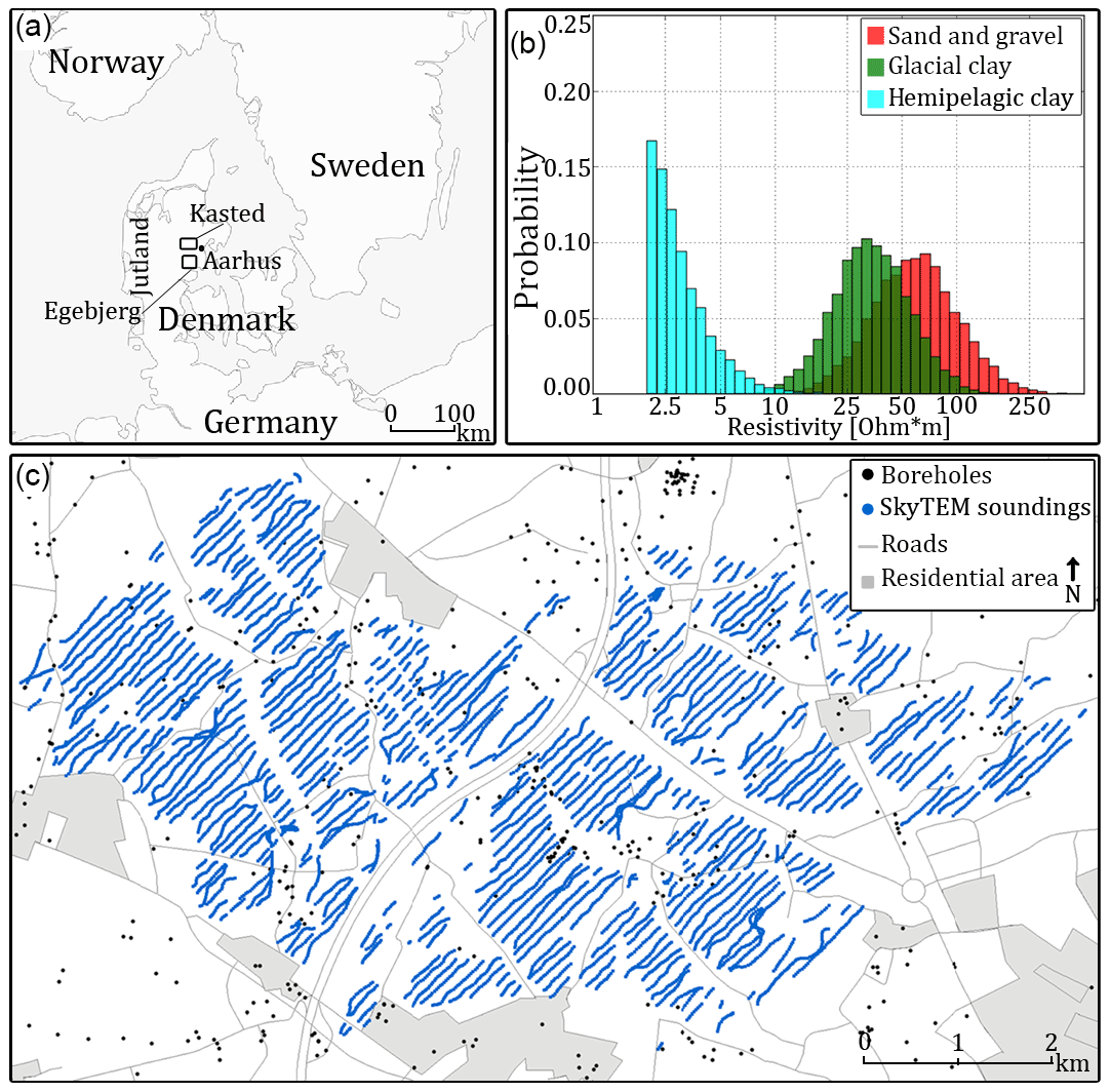
Figure 1The Kasted survey area and resistivity–hydrostratigraphic relationship histograms. (a) shows the geographical location of the Kasted survey area and the Egebjerg model used as a secondary TI. (b) shows the reconstructed resistivity–hydrostratigraphic relationship histograms for the three main hydrostratigraphic unit categories based on SkyTEM resistivity models and borehole lithology logs. (c) shows the Kasted survey with the SkyTEM sounding and borehole locations. Note that the SkyTEM soundings are sampled so densely that the dots marking each individual sounding merge into blue lines.
3.1 Multiple-point statistics (MPS)
The multiple-point statistics framework stems from the general geostatistics framework. Here, multiple-point (MP) information from a training image is used to condition simulations to probable geological patterns (Journel and Zhang, 2007). The TI thus provides a conceptual geological understanding of a given area and can be viewed as a database containing probable geological patterns, which are used to condition the MPS simulation. The choice of TI is an important step in any MPS setup and influences the realization results, as will be illustrated. The TI does not need to carry locally accurate information – i.e., the TI does not need to spatially or geographically overlap with real-world geological units – and can be purely conceptual in nature. Together with the TI, it is also possible to use geophysical datasets for constraining MPS simulations, resulting in realizations that reflect real-world regional geology. Today, MPS is a widely used tool, which is used in a variety of geoscience fields, including, but not limited to, reservoir modeling (e.g., Okabe and Blunt, 2004; Strebelle and Journel, 2001), hydrology (e.g., Le Coz et al., 2011; Hermans et al., 2015; Høyer et al., 2017), and geological modeling (e.g., de Iaco and Maggio, 2011).
3.1.1 Single normal equation simulation (snesim)
The MPS method used in this paper is known as the single normal equation simulation (snesim) framework (Strebelle, 2002), and is implemented in the Stanford Geostatistical Modeling Software, or SGeMS. The snesim framework allows for simulating a real-world categorical geological model using a TI, constrained using soft geophysical data and hard borehole data. The snesim algorithm scans the entire TI, ahead of simulation, and stores the MP information contained in the TI in a search-tree database. The MP information can then be retrieved from the database during simulation. The integration of soft geophysical data for constraining the simulations is achieved by utilizing the tau model, which will be described in detail in Sect. 3.2 (Journel, 2002; Krishnan, 2004). Here, the continuous soft data variable needs to be translated into a probability grid, describing the probability of finding a given geological unit based on the geophysical data; see Barfod et al. (2018). In order to guarantee the reproduction of geological patterns at all scales, snesim uses the multiple-grid formulation, presented by Tran (1994).
3.1.2 Reconstructing incomplete datasets using direct sampling
In the field of geoscience, we are always dealing with incomplete datasets, since we cannot sample the subsurface exhaustively. Several approaches exist for dealing with incomplete datasets, of which two general approaches can be defined. A common approach is to reconstruct incomplete datasets using geostatistical tools (e.g., Goovaerts, 1997; Mariethoz and Renard, 2010), which means that during the hydrostratigraphic modeling process no information is present in the dataset gaps. However, it is important to emphasize that the reconstructed information is not as valuable as the actual measured geophysical information. The other common approach is to just use the incomplete dataset as is. This means that no information is present in the dataset gaps during the hydrostratigraphic modeling process, which, depending on the modeling method, might result in large uncertainties.
In this study the MPS method called direct sampling (DS) is used for stochastic reconstruction of incomplete datasets (Mariethoz and Renard, 2010). The DS method uses the dataset we wish to reconstruct both as a simulation grid and a TI. This means that the patterns that are present in the incomplete dataset are inserted into the simulation grid before reconstruction. It is, according to Mariethoz and Renard (2010), important that the patterns we wish to reconstruct are actually present in the incomplete dataset, since we are borrowing the patterns from the TI, or incomplete dataset, to stochastically reconstruct the dataset. If the patterns are not present in the incomplete dataset they will, simply put, not be inferred in the reconstructed dataset. Provided that enough information on the overall patterns is available in the incomplete dataset, the DS method is a straightforward approach for reconstructing incomplete datasets.
3.2 The tau model: combining conditional probabilities
Combining information from different sources is a frequent challenge in subsurface modeling. A fundamental challenge of the research conducted in this paper was to combine conditional probabilities from different sources. In this paper we used the common tau model approach (Journel, 2002). The tau model generally combines the probability values from different sources using Bayes' theorem and a set of τ values, or τ weights, for determining how to weigh the probabilities. The choice of τ weights is subjective, and assigning these is not a trivial task. It is recommended to run a series of exhaustive tests when assigning the τ weights.
We will now briefly introduce the tau model; for more details see Journel (2002). Firstly, we define a data event, Di, as a location vector, u, and a data value. Suppose we have a set of such data events, Dii=1, …, n, and the goal is to estimate the probability that a hydrostratigraphic unit (A) is present provided all data events:
The first step is then to define the prior probability distribution, P(A). Generally the tau model can be applied to as many different probability grids as desired, but for the purpose of simplification two probability distributions are defined as follows: P(A|D1) and P(A|D2). In this study we will consider D1 and D2 as 2-D or 3-D probability grids from different sources. As an example D1 could be a probability grid from geophysical data and D2 a probability grid from borehole lithology logs. The probability grids are translated into distance grids by applying the “probability-into-distance” transform:
Then the following distance ratio is computed using the tau model expression:
where the tau values are [τ1, τ2]. The final conditional probability is computed as follows:
where the value of x is computed from Eq. (2), as follows:
3.3 Comparing simulation results
Comparing a large set of extensive 3-D models is a common problem encountered in stochastic MPS modeling. A common approach is visual comparison, which is not an objective or quantitative comparison method. Each equiprobable hydrostratigraphic model in this study contains 1 187 823 cells. Furthermore, a total of 400 MPS realizations were computed, Table 1, which makes it difficult to visually compare modeling results. This, along with advances in stochastic modeling tools such as MPS, motivated Tan et al. (2014) to develop a framework in which multiple 2-D or 3-D realizations can be compared quantitatively. The idea is to use a distance measure, which measures the distance between two realizations. Realizations which are geometrically similar have small distance values, while dissimilar realizations have a large distance value. The comparison techniques in this study are based on the principles presented by Tan et al. (2014). In this study the distances between individual realizations are based on the Euclidean distance transforms (Maurer et al., 2003). The usage of EDT as a measure for similarity will be described in more detail below. A full distance matrix is computed containing distances between each individual realization for all the different cases. The resulting 400 by 400 distance matrix is then interpreted by itself.
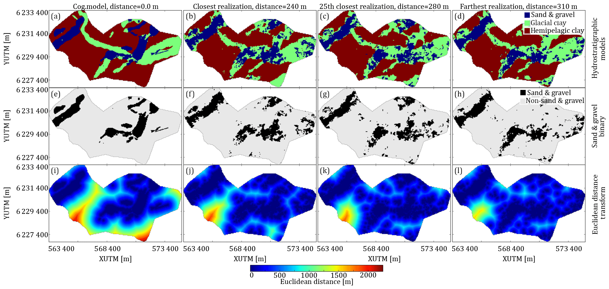
Figure 2A 2-D example of the Euclidean distance transforms (EDT) as a measure for the similarity between categorical MPS realizations. In this example a set of 50 realizations, from the basic modeling setup, are compared based on the differences in EDT for sand and gravel units. (a–d) show the hydrostratigraphic models for the TI, closest realization, 25th closest realizations, and farthest realization, respectively. (e–h) show, in the same order as above, the binary images of the sand and gravel units of the 2-D hydrostratigraphic model layers. (i–l) show, in the same order as above, the Euclidean distances layers computed from the 2-D sand and gravel binary layers.
3.3.1 Ensemble mode ratio maps (EMR maps)
The visual comparison can be helped by creating so-called ensemble mode ratio maps, or EMR maps. The idea is to create a summary map portraying the mode ratio of a given ensemble of models, ranging between 1∕K and 1, where K is the number of hydrostratigraphic categories. The EMR maps describe the certainty of the simulation based on the resulting realization ensemble. If the EMR map shows a value of 1, then every single realization in the present ensemble has simulated the same category or, in this case, hydrostratigraphic unit. On the other hand, if the EMR map shows a ratio of 1∕K the ensemble of realizations shows equal probability for each of the K categories. Each realization is equiprobable, and the EMR values of the categorical variables are computed from the probability distribution of a given cell with location, u. The probability that the attribute S is equal to sk, Pk(u), is computed as follows:
where N is the number of realizations, sk is the state of attribute S for which we are currently computing the probability, and sk,i(u) is the state of the attribute at location u and for the ith realization. The EMR values for a given cell, u, can then be computed as follows:
where Pk(u) denotes the probability for category k at location u computed using Eq. (6).
The EMR values are then computed for each grid cell using Eqs. (6) and (7), which, simply put, is the occurrence ratio of the mode category of a given ensemble containing a given number of realizations, Nreals. In other words, at a given location, u, if 45 out of 50 realizations yield the same category, then the EMR value is 0.9, and the ensemble certainty for the given cell is high. On the other hand, with three possible lithological categories, i.e., K=3, the lowest possible certainty is , which means there is an equal probability of occurrence for each lithological category. This means that , and therefore at the given location, u, the and the simulation is uncertain.
3.3.2 Euclidean distance transforms (EDT) – measuring similarity between 3-D hydrostratigraphic realizations
The hydrostratigraphic realizations are categorical and contain three hydrostratigraphic units. Comparing two realization grids, they first need to be transformed from a categorical grid into continuous Euclidean distance grids by using EDT (Maurer et al., 2003). The two 3-D EDT grids are then compared by calculating the average difference in the respective grids. Similar images have a small average EDT distance, and dissimilar images have a large average EDT distance. The EDT computes the Euclidean distances for all locations of a binary grid, i.e., a grid containing only two states (codes 0 and 1). The EDT map is simply the Euclidean distance of the medium depicted by the state code 1, i.e., for grid cell at location u:
where v is a set of grid cells with a state code equal to 1.

Figure 3A schematic diagram presenting the conversion of the lithological logs into probability logs for the three hydrostratigraphic units: sand and gravel, glacial clay, and hemipelagic clay. Step 1: the lithology log is translated into a hydrostratigraphic log. Step 2: the hydrostratigraphic logs are resampled according to the vertical modeling grid intervals and an interval probability is calculated for each of the hydrostratigraphic units.
The dEDT implementation presented by Maurer et al. (2003) uses a computationally favorable method for computing the exhaustive EDT at all locations in a binary grid.
To illustrate the dEDT approach for comparing realizations a 2-D example case is presented. The basic modeling setup contains 50 realizations, i.e., Nrealizations=50, which are going to be compared to the cognitive model, which in this case also happens to be the TI. The 2-D example is created by selecting the horizontal cross section at 20 m b.s.l., for each of the 50 basic modeling setup realizations and the single cognitive geological model (Fig. 2a–d). Each of the 2-D layers are transformed into 2-D binary layers, portraying sand and gravel as the main variable, and glacial clay and hemipelagic clay as a background variable (Fig. 2e–h). The 2-D binary layers are then translated into 2-D dEDT layers by using Eq. (8) to exhaustively compute the dEDT at each grid cell for all of the 50 realizations. The resulting dEDT layers, of which three are seen in Fig. 2i–l, are used to compute an average Euclidean distance between each realization, mr,i, and the cognitive geological model, mcog:
where , with N being the number of realizations, which in this case is N=50, and M being the number of cells in the simulation grid, or in this case, the 2-D layer. The ΔdEDT, Eq. (9), then describes the average difference of the distance to the nearest active cell in the binary grid. The 50 realizations are then ranked by the average Euclidean distance differences, ΔdEDT, as seen in Fig. 2, where the realization which is closest to the cognitive geological model (Fig. 2b, f and j) has a ΔdEDT value of 240 m, the realization which was ranked 25th closest (Fig. 2c, g and k) has a ΔdEDT value of 280 m, and lastly the realization which was farthest (Fig. 2d, h and l) has a ΔdEDT value of 310 m. It should be noted that the ΔdEDT computation, described by Eq. (9), is not limited to comparing a realization to a cognitive model and can in fact be used to compare any pair of 3-D categorical models. In fact, a generalized version of Eq. (9) can be defined as follows:
where the number of cells in model-A, mA, must be equal to the number of cells in model-B, mB, i.e., .
From this point forward we leave the 2-D example behind and will from here on only consider ΔdEDT computations on 3-D hydrostratigraphic grids. Furthermore, the ΔdEDT computations are carried out on a set of three binary grids, one for each of the three hydrostratigraphic categories. The distance value between two hydrostratigraphic grids is the summed distance for each of the three hydrostratigraphic categories, ensuring that the distance values reflect the complexities related to each of the hydrostratigraphic categories.
3.3.3 Evaluating the distance matrix
The average Euclidean distance difference, ΔdEDT, from here on referred to as the distance between two realizations, is exhaustively computed between all realizations and compiled into an exhaustive 400 by 400 distance matrix. The distance matrix, D, contains all distance values between all hydrostratigraphic realizations computed using Eq. (9) and is defined as follows:
where , with N being the number of realizations. The distance matrix, D, can be evaluated directly by comparing the distances between individual realizations to each other. Another option is to summarize the distance matrix in a table representing the distances between the different cases. This is achieved by organizing the distance matrix according to which case they belong to. In this study the distance matrix is sorted according to the order of the individual cases, as in Table 1. The distance matrix can then be summarized by computing the average distance for each group of realizations pertaining to a specific case. The concepts of distance variability and distance to cognitive model were presented by Barfod et al. (2018) and are also used here. The concept is that the variability pertaining to a specific case can be determined by computing the average of the distances of the 50 realizations for a given case ensemble. Another measure is the distance to the cognitive model. The distances between all realizations and the cognitive model are computed, and this provides a reference point to which the realizations are compared.
The Kasted dataset used in this study is comprised of a dense geophysical dataset acquired using the SkyTEM system (Sørensen and Auken, 2004), borehole lithology logs and a cognitive geological model (Høyer et al., 2015). We show how uncertainty related to resistivity data, measured with the SkyTEM system, and borehole lithology logs influences the hydrostratigraphic modeling realizations. Two readily available MPS tools are showcased. The first tool is the direct sampling method for reconstruction of incomplete datasets (Mariethoz and Renard, 2010). The other MPS tool is the single normal equation simulation, which is used for stochastic hydrostratigraphic modeling (Strebelle, 2002). The MPS modeling setup is similar to the one presented by Barfod et al. (2018). However, the goal of this study is different. The study is divided into a total of six cases, or eight sub-cases, which are designed to study how perturbations of the underlying MPS setup affect the hydrostratigraphic realizations using snesim and study the propagation of uncertainties into the hydrostratigraphic models. First the basic case (case 0), from which the other cases are perturbed, uses a hydrostratigraphic simplification of the 3-D cognitive model of the Kasted area as a TI, the gap-filled SkyTEM data present as smooth inversion models as soft data, and the borehole lithological logs as hard data. Then, in case 1, the TI is substituted by two other TIs. The cases 2 and 3 are related to the SkyTEM data, where the incomplete SkyTEM data and sSCI inversion models are used, respectively. The influence of the boreholes is studied in case 4 either leaving out boreholes as hard data or changing them into soft data. Finally, in case 5 the SkyTEM data are not used. In other words, one of the overall goals of this study is to improve the Kasted model by using stochastic ensemble modeling to quantify the uncertainty of the model, such as suggested by Ferré (2017) and Pirot (2017). Further details on the individual cases follow in the coming sections and Table 1 summarizes each case. First of all, the model discretization and parameterization as well as construction of hard and soft data grids are described.
The Kasted model covers an area of 12 km by 7 km, discretized on a modeling grid with 229 by 133 by 39 cells, containing a total of 1 187 823 cells. Each cell has a size of 50 m by 50 m by 5 m. It is parameterized into three hydrostratigraphic units, listed as follows.
-
Sand and gravel: a combination of coarse lithological units, including sand till, meltwater sand, gravel and pebbles of glacial origin, late glacial freshwater sand, and postglacial freshwater sand.
-
Glacial clay: this category contains silty and sandy clays, including clay till and meltwater clay of glacial origin.
-
Hemipelagic clay: a combination of fine grained conductive clays, containing the extensive and homogeneous hemipelagic Paleogene and Oligocene clays found in Denmark.
These three categories serve the purpose of simplifying the geology of the Kasted area. The Kasted survey lithology logs reveal a combination of 59 geological categories, which are translated into a set of hydrostratigraphic logs (Step 1, Fig. 3) using these hydrostratigraphic categories. Similarly, the 42 geological units in the cognitive geological model are divided into the three abovementioned categories (Fig. 4a). The vertical proportions of the three-category hydrostratigraphic Kasted model can be viewed in Fig. 5a.
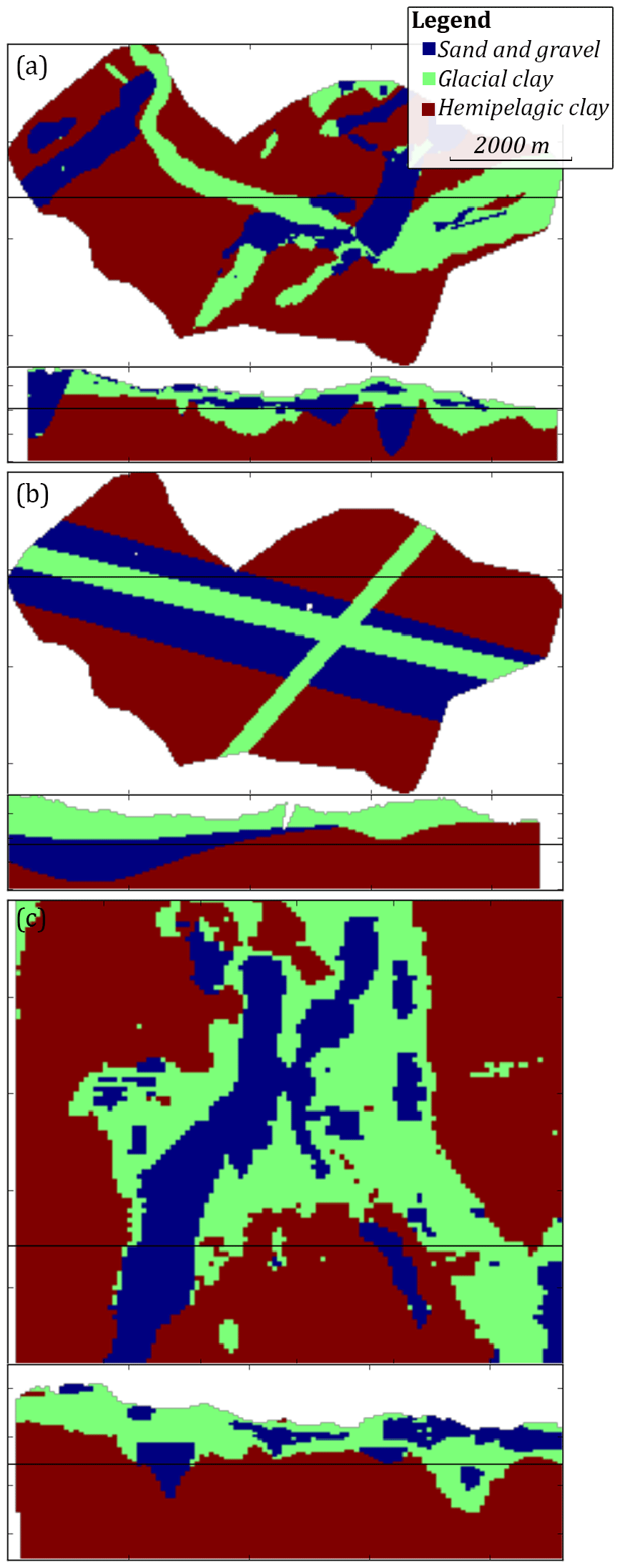
Figure 4An overview of the training images (TIs) which are used during MPS simulation. A horizontal slice and vertical cross section is presented for each TI, portraying the hydrostratigraphic architecture; (a) shows the Kasted TI, (b) shows the conceptual TI, and (c) shows the Egebjerg TI, which is generally larger than the Kasted model.
The borehole lithology logs need to be assigned to a 3-D grid, which is carried out in three overall steps. The first step is to translate the borehole lithology logs into hydrostratigraphic logs using the above mentioned three categories; Step 1, Fig. 3. The second step is then to divide the hydrostratigraphic logs into intervals identical to the vertical intervals of the model grid. At each resampled interval a probability value is directly calculated for each hydrostratigraphic unit; Step 2, Fig. 3. The probability is simply the percentage of the given unit, which is present within the interval. Finally, the last step is to assign the hydrostratigraphic probabilities to a grid. The probability values are assigned to the grid cell in which the given hydrostratigraphic log is present. On the rare occasion that multiple logs are present within a given cell, the probabilities are combined accordingly to one representative probability value. The end result is a grid containing the borehole probability values of each hydrostratigraphic unit: sand and gravel, glacial clay, and hemipelagic clay. It is common to view borehole lithology logs as hard information, or ground truth. The borehole probability grid can therefore be translated into a hard data grid, by assigning the most probable hydrostratigraphic unit in each grid cell.
The 1-D SkyTEM resistivity models are assigned to a 3-D grid, identical to the modeling grid. The first step is to fill all grid cells containing a resistivity model. This is carried out using block kriging and results in an incomplete resistivity grid of block average resistivities (Fig. 6a). The second and final step is to stochastically reconstruct the incomplete resistivity grid using DS stochastic reconstruction (Mariethoz and Renard, 2010) (Fig. 7). The reconstruction procedure was originally presented by Barfod et al. (2018); however, we have made some improvements for this study. Originally, a simple kriging estimation approach was used to assign the resistivity models to a 3-D modeling grid. This resulted in an incomplete resistivity grid, which contained resistivity information not only pertaining to grid cells containing a SkyTEM sounding; i.e., the resistivity grid had already been partly reconstructed in the proximity of the geophysical soundings. To avoid this, block kriging estimation was used instead. The block kriging method is also a variogram-based estimation method, which estimates the average value of a rectangular block (Goovaerts, 1997). For more details on reconstructing incomplete resistivity grids see Barfod et al. (2018).
The SGeMS snesim framework utilizes the tau model for soft data conditioning (Journel, 2002), which requires the translation of resistivity grids into probability grids. This requires information on the regional resistivity–hydrostratigraphic relationship. Such knowledge is not always available, but if enough boreholes and electromagnetic geophysical data are available, the framework for studying the resistivity–hydrostratigraphic relationship, presented by Barfod et al. (2016), can be used to create a set of histograms. The resistivity–hydrostratigraphic histograms, Fig. 1b, are compiled from available hydrostratigraphic logs and SkyTEM resistivity models and are presented in more detail in Barfod et al. (2016, 2018). The estimated histograms (Fig. 1b) are then used to directly translate each resistivity value, in a given resistivity grid, into three probabilities, one for each hydrostratigraphic unit.
The general MPS workflow can be summarized in seven overall steps as follows:
-
Using block kriging, the SkyTEM resistivity models are assigned to a 3-D grid identical to the Kasted model grid.
-
The incomplete resistivity grids (Fig. 6a) are stochastically reconstructed using direct sampling (Fig. 7a). The result is an ensemble of 50 equiprobable reconstructed resistivity grids.
-
The reconstructed resistivity grids are translated into probability grids using the resistivity–hydrostratigraphic relationship histograms (Fig. 1b).
-
The borehole lithology logs are translated into hydrostratigraphic logs; Step 1, Fig. 3.
-
The hydrostratigraphic logs are resampled and three probability values, one for each hydrostratigraphic unit, are directly computed at each resampled interval; Step 2, Fig. 3.
-
The borehole probabilities are assigned to a grid identical to the cognitive Kasted model grid.
-
The borehole probability grid is translated into a hard data grid, by assigning the most likely hydrostratigraphic unit to each grid cell.
A total of 400 realizations are created, with 50 realizations per sub-case (Table 1). In snesim a random number seed needs to be manually selected for each realization to initialize the random number generator and in particular define a random path through the modeling grid. The random seed convention chosen in this paper was to apply the same random seed vector to each sub-case. The vector contains 50 linearly increasing random seed numbers, ensuring consistency when comparing realizations from the individual sub-cases.
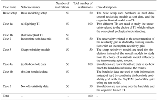
Table 1An overview table showing information on the MPS cases along with information on the number of realizations for each case or sub-case, and a brief description of each case.
4.1 Basic modeling setup
The basic modeling setup is designed to act as the base from which all other cases are built. The different sub-cases are simply modified versions of the basic modeling setup, each designed to study how modification to the base setup relates to hydrostratigraphic MPS modeling. The basic modeling setup uses the borehole data as hard information, SCI models with smooth inversion constraints as soft data, and the cognitive hydrostratigraphic Kasted model as a TI (Fig. 4a), for which the global proportions are listed in Table 2 and vertical proportions are displayed in Fig. 5a.
4.2 Case 1 – conceptual geological understanding
The basic modeling setup uses the actual cognitive geological model of the Kasted survey area as a TI (Høyer et al., 2015). In Denmark, it is common practice to build 3-D cognitive geological models of the near-subsurface. Many cognitive models exist and are publicly available. Such models can easily be adapted and used as 3-D TIs to simulate new survey areas, provided the geological settings are similar. Case 1 is divided into two sub-cases. The first sub-case, case 1a, uses the basic setup, but, in place of the cognitive Kasted model, the cognitive geological model of the Egebjerg area (Fig. 1a) is used as a TI (Fig. 4c). The geologic setting in Egebjerg is relevant since it is partly dominated by a buried valley complex (Jørgensen et al., 2010).
The Egebjerg model consists of a total of 72 geological units which are categorized accordingly to reflect the three hydrostratigraphic units of the Kasted hydrostratigraphic model. Egebjerg additionally contains undesired features, such as local Miocene complexes. Two such local geological environments, which do not reflect the geological setting of the Kasted area, are present. One is found south of the buried valley complex and the other to the west. By cropping the model and rotating it 90∘ counterclockwise, a relevant TI without undesired geological architecture is produced (Fig. 4c); this is referred to as case 1a. It is clearly seen by comparing Fig. 4a and c that the Kasted and Egebjerg TIs are different. The Kasted TI is smaller and contains smooth geological features, while the Egebjerg model is larger and contains coarse, block-like geological features. The important features, in relation to hydrostratigraphic modeling, are the buried valley complexes, which are present in the Egebjerg model (Fig. 4c). The global proportions of the Egebjerg TI (Table 2) are similar to the ones found in the Kasted TI. However, the vertical proportions of the Egebjerg TI (Fig. 5c) are different, especially in the upper part of the TI where glacial clay units dominate.
Table 2The global proportions related to each of the three TIs presented in Fig. 4.
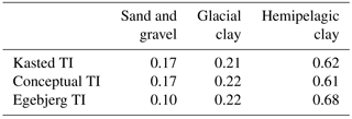
The second sub-case, case 1b, utilizes a purely conceptual TI. The conceptual TI is created by using a set of hyperbolic secant functions to populate a 3-D matrix and is purely mathematical in nature. The conceptual TI can be seen in Fig. 4b and is designed to have three overall buried valleys eroded into a hemipelagic clay substratum. There are two narrow and shallow glacial clay valleys, and a broad and deep sand and gravel valley. One of the glacial clay valleys is a younger valley that is eroded into the older sand and gravel valley and they run roughly parallel to each other. The last glacial clay valley is almost orthogonal to the other valleys, and also erodes into the sand and gravel valley. The upper part of the TI contains a cover layer of glacial clay (Fig. 5b). The simple conceptual TI is designed to contain the main geological architecture of the Kasted area, namely the buried valley complexes. The sand and gravel valley, trending west–northwest to east–southeast, was chosen on purpose to study what happens when oversimplified and smooth MP information is added to a TI. The global proportions of the conceptual TI are consistent with the other TIs, while the vertical proportions for sand and gravel and glacial clay units show a significantly different pattern (Fig. 5b).
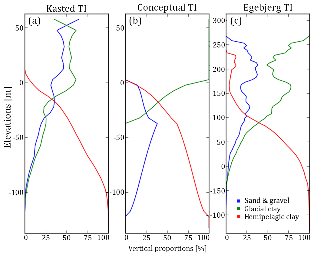
Figure 5The vertical proportions of the three training images for each of the hydrostratigraphic categories, where (a) portrays the Kasted TI, (b) the conceptual TI, and (c) the Egebjerg TI.
4.3 Case 2 – incomplete soft data
During reconstruction of the resistivity grid, it is assumed that the patterns in the incomplete dataset contain information regarding the content of the dataset gaps. This is true only when the incomplete grid contains a sufficient amount of data. Sufficient, in this case, means that the parameter space is sampled densely enough to reflect the patterns we wish to reconstruct (Mariethoz and Renard, 2010). If the grid is too sparse, then limited or no information which can help reconstruct missing patterns is present. Signs of mediocre data density are seen in the incomplete grids (Fig. 6a). Artifacts from the DS reconstruction are present in the completed resistivity grids. The resistive valley to the west in the horizontal slices and vertical cross sections in Fig. 7a and b reveal a striated pattern. An alternative to reconstructing the resistivity grid beforehand is to use the incomplete resistivity grids for simulation, meaning no information is present in the resistivity dataset gaps. Grid cells containing a resistivity model are translated into three probability values using the resistivity–hydrostratigraphic relationship histograms (Fig. 1b, 6b–d). Areas without soft resistivity data rely on the TI during simulation, emphasizing the fact that no actual information is present between soundings. The overall setup is identical to the basic setup; the only difference is the reconstructed soft data grids are interchanged for the incomplete soft data grid (Fig. 6b–d).

Figure 6A presentation of the incomplete resistivity grid. Each grid is portrayed as a horizontal slice at 20 m b.s.l. and a vertical cross section intersecting at YUTM 6 230 100 m. (a) shows the resistivity grid which is translated into three probability grids using the resistivity–hydrostratigraphic relationship histograms (Fig. 1b). Grid cells without SkyTEM soundings are not assigned a probability value. (b–d) show the sand and gravel, glacial clay, and hemipelagic clay probability values, respectively.
4.4 Case 3 – choice of resistivity model
The choice of inversion algorithm results in different SkyTEM resistivity models. The purpose of this case is to study how using sSCI (Vignoli et al., 2015) models influences the modeling results. A common inversion approach is SCI, where a smooth regularization is used (Constable et al., 1987). Such resistivity models have a smooth transition from resistive to conductive features, and vice versa. Geological layer boundaries are rarely smooth in nature, meaning such soft transitions in resistivities seldom reflect reality. Furthermore, extreme resistivity values are not presented correctly in the smooth model inversions. Vignoli et al. (2015) propose an alternative SCI approach, employing a minimum gradient support regularization term instead. Such sSCI models produce resistivity models with sharp layer boundaries and a better representation of extreme values. The setup in case 3 is identical to the basic setup, except that the SCI models are interchanged for sSCI models. The DS grid reconstruction is then conducted on the sSCI models, which are then translated into probability grids. Finally, these grids are used as soft data for simulation using the snesim method.
The sharp resistivity models are different from the smooth models, but no particularly sharp layer boundaries are reflected in the reconstructed resistivity grid (Fig. 7b).
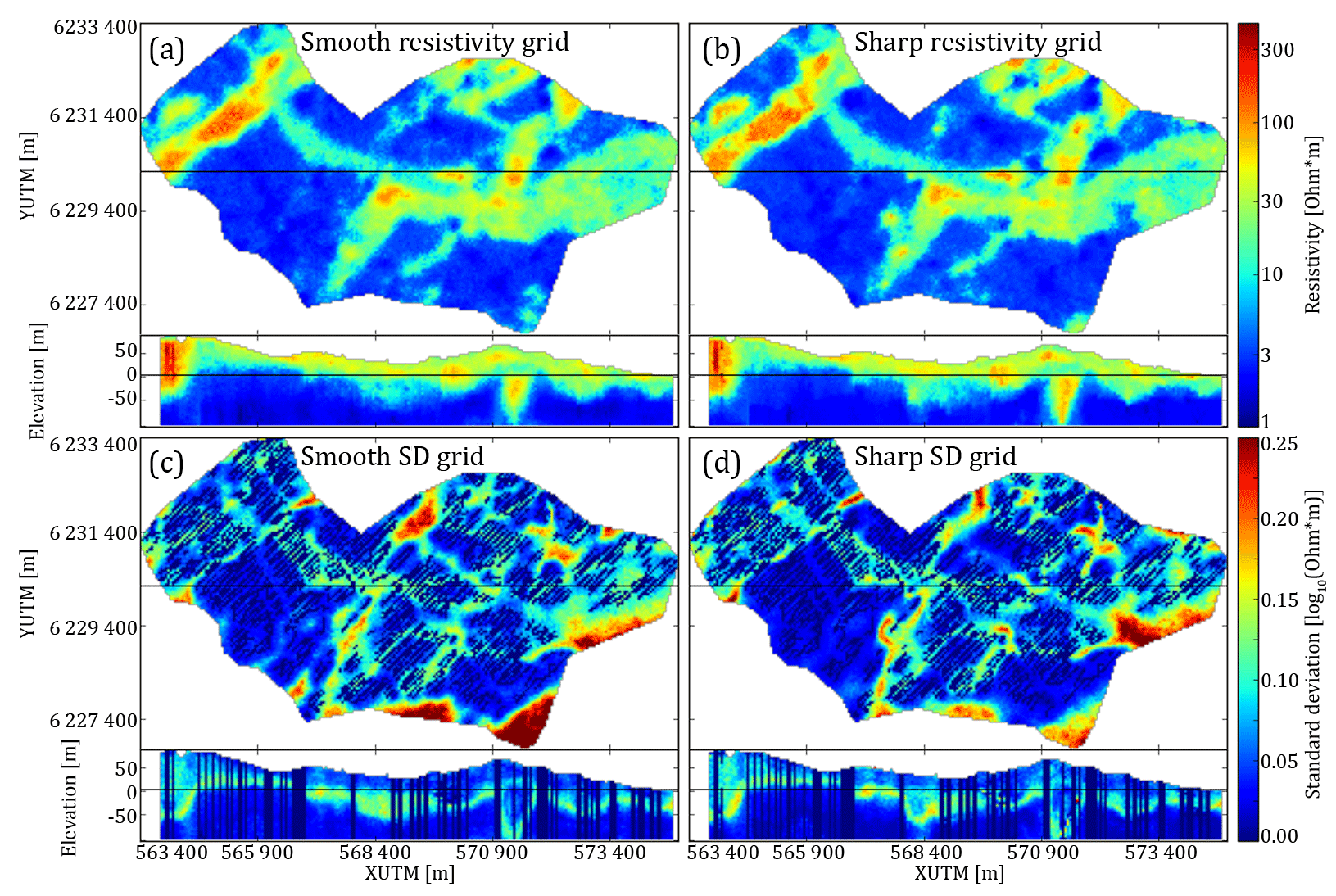
Figure 7An overview of the key differences between reconstructing the resistivity grid using smooth and sharp inversion resistivity models. Each grid is portrayed as a horizontal slice at 20 m b.s.l. and a vertical cross section intersecting at YUTM 6 230 100 m. (a) shows the smooth reconstructed resistivity grid. (b) portrays the sharp reconstructed resistivity grid. (c) shows the standard deviation calculated from 50 stochastic reconstructions of the smooth resistivity grid. (d) shows the standard deviation calculated from 50 stochastic reconstructions of the sharp resistivity grid.
One of the obvious differences is found in the resistivity patterns of the sand and gravel valley to the far west of the survey area. The valley itself is not significantly different; however, the small resistive patch, west of the large valley, is more pronounced in the sharp model and has an overall more pronounced fingerprint (Fig. 7b). The sharp resistivity models better estimate the true bulk resistivity values of specific geological units, such as the resistive patch accentuated here. The ensemble standard deviation grid, Fig. 7c and d, shows a general reduction in the ambiguity of the reconstructed sharp resistivity models. This is clear from the reduction areas with large standard deviation, shown in red colors, which are overall reduced in size.
4.5 Case 4 – borehole lithology logs
This case is dedicated towards how the borehole data are handled and how they influence the hydrostratigraphic modeling results. The hard borehole data are normally sparse, relative to geophysical data. Boreholes are commonly considered ground truth since they directly sample the subsurface sediments or petrological units. This case is divided into two sub-cases. The first sub-case, case 4a, portrays what happens when hard data are not included in the snesim simulation. The model setup is therefore identical to the basic MPS setup, but without including the borehole data.
The second sub-case, case 4b, incorporates the borehole lithology logs as soft data. The certainty of a lithological log varies depending on a range of factors, e.g., drilling method, the purpose of the borehole, and sampling frequency (e.g., Barfod et al., 2016; He et al., 2014). The hydrostratigraphic probability logs, introduced in the basic modeling setup (Step 2, Fig. 3), are utilized in place of the hard borehole grid. The boreholes are assigned a lateral footprint, so the information is not only found at the borehole locations. The borehole footprint is assigned by creating a grid where the borehole probability values have been estimated in a radius of 200 m around each borehole using simple kriging with a search radius of 200 m and a mean of , where K is the number of unique hydrostratigraphic units (Fig. 8d–f) (for additional information see Sect. A1 in the Appendix). The tau model is then used to combine the SkyTEM (Fig. 8a–c) and borehole (Fig. 8d–f) probability grids (e.g., Journel, 2002; Krishnan, 2004; Remy et al., 2014). The first step is then to define the prior probability distribution, P(A), which in this case is the vertical proportion taken from each layer of the cognitive Kasted TI (Fig. 5a). Then the probability distributions are defined as follows: P(A|Dr) and P(A|Db), where Dr is the resistivity probability grid and Db the borehole probability grid. The 3-D probability grids are translated into distance grids by applying the probability-into-distance transform and computing the distance ratio using Eqs. (2) and (3), where the tau values were assigned based on a series of exhaustive tests. The final tau values were selected based on the criteria that the transitions in areas where both borehole and resistivity information is available should be as smooth as possible in the resulting combined probability grid, as seen in Fig. 8. Based on the tests, the resulting tau values were . The final conditional probability was computed using Eq. (4) and resulted in the three hydrostratigraphic probability grids, as seen in Fig. 8g–i. The combined probability grids replace the smooth probability grids used in the basic setup.
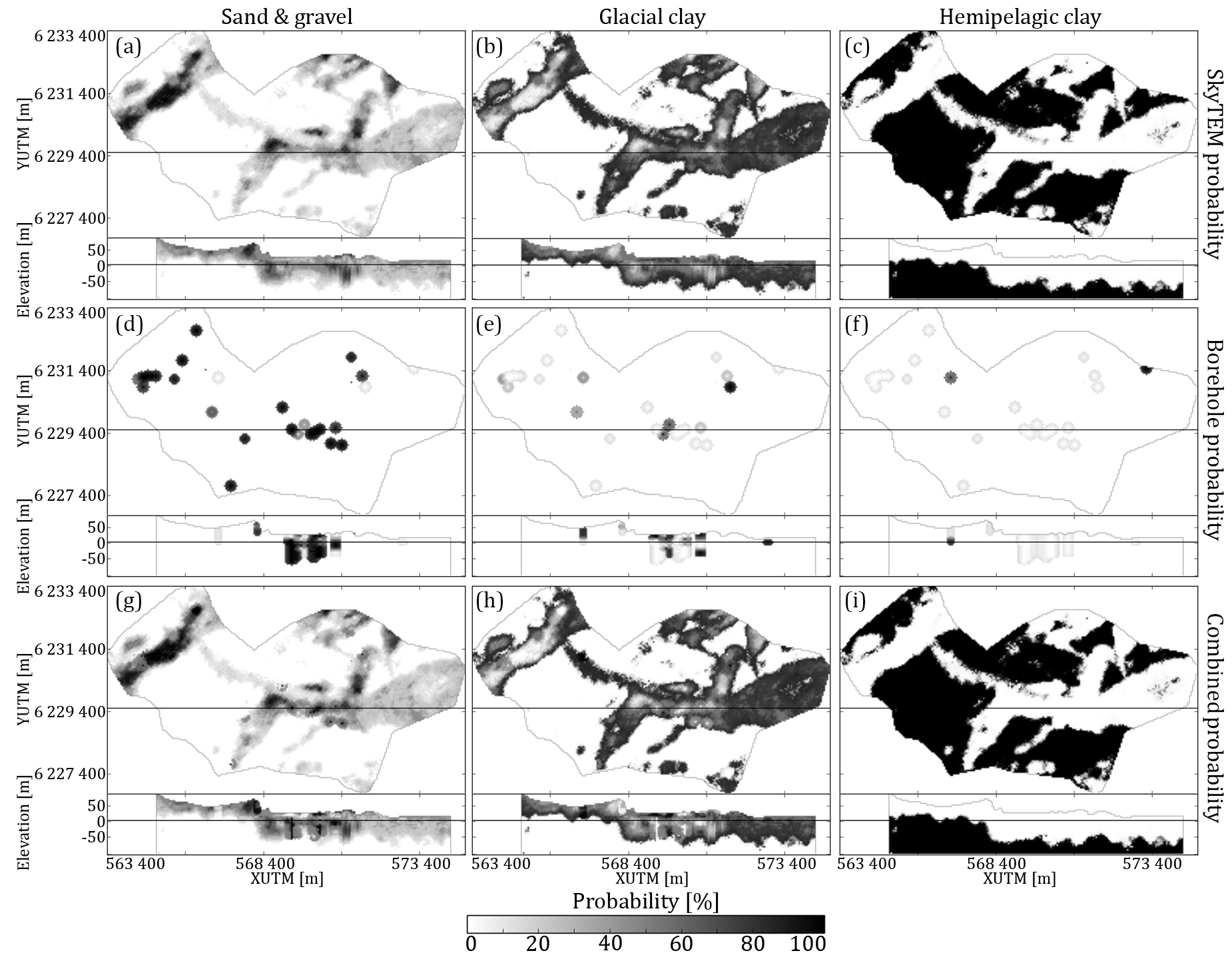
Figure 8A visual representation of the tau model procedure for combining the soft resistivity and borehole grids. Each grid is portrayed as a horizontal slice at 20 m b.s.l. and a vertical cross section intersecting at YUTM 6 230 100 m. (a–c) show the sand and gravel, glacial clay, and hemipelagic clay probability maps, respectively, for one DS reconstructed resistivity grid; d–f show the 200 m radius kriged borehole probability; and (g–i) show the combined resistivity grid, which has been combined using a tau model with the values [2, 1].
4.6 Case 5 – excluding the soft resistivity data
The final case, case 5, illustrates the consequences of not including the soft SkyTEM resistivity information in the MPS simulation routine. The basic setup is simply run without the inclusion of soft data; i.e., the setup only uses the cognitive Kasted TI and hard borehole information.
5.1 Visual comparison of hydrostratigraphic realizations and ensemble mode ratio maps
For each of the presented cases two hydrostratigraphic realizations are presented (Fig. 9), along with an EMR map (Fig. 10). The EMR maps show the occurrence ratio of the most likely simulated category for each grid cell based on 50 realizations. The two realizations and EMR map of the basic modeling setup, Figs. 9a and 10a, reveal the same overall trends as the cognitive geological model, Fig. 4a: namely the western sand and gravel valley striking ∼ N40∘ E, the glacial clay valley striking ∼ E30∘ S, the large mixed sand and gravel and glacial clay valley striking ∼ N20∘ E to the south, and the small subsidiary glacial clay valley striking ∼ N50∘ E to the south. However, even though the main hydrostratigraphic architecture of the cognitive geological model is similar, there are still differences between the snesim realizations and the cognitive geological model. The cognitive model shows clear-cut, smooth, and ordered hydrostratigraphic units. The basic modeling setup realizations reveal sporadic and random patterns. The sand and gravel units are placed in small lumps throughout the glacial clay units, but are not present within the homogenous hemipelagic clay. Patches of uncertain glacial clay units are, however, found in the homogeneous hemipelagic clay, especially in the southeast corner of the Kasted survey area (Figs. 9a, 10a). The same sporadic picture is seen in the vertical slices of the realizations (Fig. 9a), although here an additional trend is revealed. The sand and gravel valley to the far west and at XUTM 570 900 m is not consistently filled with sand and gravel (Fig. 9a) as in the cognitive geological model (Fig. 4a). Furthermore, the EMR map reveals that the valley margins are subject to a larger degree of ambiguity (Fig. 10a); in fact at some locations the rEMR value is close to 1∕3, which means that for the model ensemble the occurrence of either hydrostratigraphic unit is possible.
The case 1a realizations (Fig. 9b, 10b), which use the Egebjerg TI (Fig. 4c), show the same overall trends as in the basic modeling setup. The subset of buried valleys mentioned above is present; however, an obvious difference is the coarse and block-like appearance of the case 1a realization ensemble. This appearance is similar to the block-like appearance of the Egebjerg TI (Fig. 4c). Furthermore, the horizontal slice of the realizations and EMR map reveals that the glacial-clay-dominated area to the east has a generally larger occurrence ratio and is thus more certain. The realizations are clearly influenced by the choice of TI, especially when case 1b is also considered (Fig. 9c). The hydrostratigraphic realizations of case 1b (Fig. 9c, 10c) clearly depict the same overall buried valley trends, but the valleys in the central part of the model are largely filled with the opposite of the valley filling hydrostratigraphic units. Furthermore, the occurrence ratio seems quite low in certain areas, such as to the south of the model, which means the ambiguity has increased. Finally, the realizations also reveal an absence of small-scale patterns, which corresponds to the conceptual TI that only contains homogenous hydrostratigraphic units.
The importance of reconstructing the incomplete resistivity grid is seen in case 2 (Fig. 9d, 10d). The two realizations in Fig. 9d show the main buried valley features, e.g., the western sand and gravel valley. However, the hydrostratigraphic units are sporadic, especially in areas with no data. Patches of sand and gravel and glacial clay are randomly spread throughout the presented horizontal slice and vertical cross section (Fig. 9d). The EMR map also reveals an increase in low occurrence ratios in areas without soft data (Fig. 10d).
The uncertainty related to the choice of geophysical modeling procedure is portrayed by case 3. Here, snesim realizations are constrained to sharp resistivity models. Generally, the realizations (Fig. 9e) are quite similar to the basic modeling setup realizations (Fig. 9a). However, a key difference is the significant reduction or absence of patches of glacial clay in the homogeneous hemipelagic clay. In fact only one patch is found in the first realization (Fig. 9e) in the southwest corner, while it is not present in the second realization, and the EMR map further reveals a reduction of the occurrence ratios generally, especially along the southern margin of the realizations (Fig. 10e).
Case 4 shows the influence that the hard data have on the hydrostratigraphic realizations in two sub-cases: case 4a, where snesim simulations are run without hard data; and case 4b, where the borehole data are treated as soft information. Fig. 9f and g shows two hydrostratigraphic realizations without hard data and with soft borehole data, respectively. These realizations do not differ significantly from the basic modeling setup realizations and in fact are quite similar. One key difference is the central glacial clay valley striking ∼ E30∘ S, which does not contain any sand and gravel to the west (Fig. 9f and g). The EMR maps reveal that without boreholes (Fig. 10f) the occurrence ratios generally decrease, making the realizations more ambiguous. The usage of the borehole data as soft information also seems to reduce the occurrence ratios compared to the basic modeling setup. Generally, leaving out the borehole data, or treating it as soft data, results in local changes in areas with a high density of boreholes.
The final case, case 5, illustrates the importance of the SkyTEM soft data. The snesim simulations are run using only hard data and the cognitive geological model as a TI. The output realizations (Fig. 9h) portray smooth and large-scale hydrostratigraphic units. The hydrostratigraphic architecture of the buried valleys is not reflected. However, the sand and gravel valley, to the west, does seem to protrude slightly in the realizations (Fig. 9h) and the EMR map reveals a significant decrease in the occurrence ratio and thus an increase in the ambiguity of the model ensemble (Fig. 10h).

Figure 9Each case is displayed by two realizations: realization no. 1 of 50 and realization no. 30 of 50. Each realization is portrayed as a horizontal slice at 20 m b.s.l. and a vertical cross section intersecting at YUTM 6230100 m. (a) shows the realization results for the basic modeling setup, (b) shows the realization results for case 1a, (c) shows the realization results for case 1b, (d) shows the results for case 2, (e) shows the results for case 3, (f) shows the results for case 4a, (g) shows the results for case 4b, and (h) shows the results for case 5. For more details on individual cases the reader is referred to Table 1.
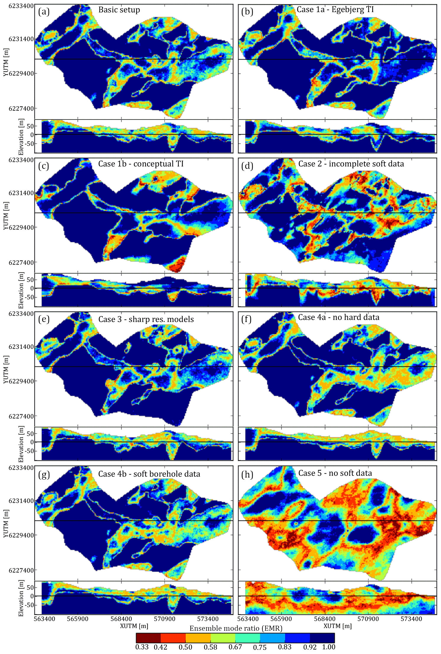
Figure 10A presentation of the ensemble mode ratio (EMR) maps, computed for the different case ensembles of hydrostratigraphic models. Each EMR map is presented as a horizontal slice centered on 20 m b.s.l. and a vertical cross section intersecting at YUTM 6 230 150 m. (a–h) present the EMR-type uncertainty map for each of the different cases, which are summarized in Table 1. The EMR values portray how certain the ensemble of MPS realizations are; i.e., if then the realization is uncertain, and we have equal probability of finding either hydrostratigraphic unit since %. On the other hand, if rEMR=1, then each realization of the given ensemble contains the same hydrostratigraphic unit at the given grid cell.
5.2 Quantitative comparison using differences in object-based Euclidean distances as a measure for similarity
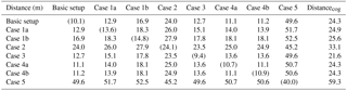
The distances between each of the 400 realizations have been computed using Eqs. (8) and (10). The full distance matrix is presented in Fig. 11a. The distances between each realization and the cognitive geological models have also been computed and plotted in Fig. 11b. To aid the interpretation of the distance matrix and distances to the cognitive model a summary table, Table 3, has been compiled.
The basic modeling setup constitutes a common snesim setup, with the geophysical data as soft data, boreholes as hard data, and a 3-D geological conceptualization encased in a TI. The ensemble average variability is computed according to the equations presented by Barfod et al. (2018), and the resulting ensemble average variability is 10.1 m, with an average distance to the cognitive model of 24.3 m. This means that the Euclidean distance mismatch between the individual realizations related to basic modeling setup is 10.1 m, and the average difference in Euclidean distance to the nearest active cell between the realizations and the cognitive model was 24.3 m.
The 3-D geological conceptualization contained in the TI influences the final hydrostratigraphic realizations as illustrated in case 1, which is divided into two sub-cases: case 1a and case 1b. In case 1a, using a 3-D cognitive geological model from the Egebjerg area as a TI for hydrostratigraphic simulation increases the average distance to the cognitive model to 24.9 m (Fig. 11a, Table 3). Furthermore, the average variability has increased to 13.6 m (Fig. 11b, Table 3). The other sub-case revolves around using an entirely conceptual geological model as a TI. The conceptual TI was designed to reflect the overall geology, yet still contains some bias. The results reflect the bias, with increased distances to the cognitive geological model, which are now centered on 25.6 m (Fig. 11a, Table 3). The ensemble variability has increased to 14.8 m (Fig. 11b, Table 3).
The importance of proper reconstruction of the incomplete resistivity grid is illustrated in case 2, where the incomplete resistivity grid was used for simulation. The resulting realization ensemble has a large ensemble variability centered on 24.1 m (Fig. 11a, Table 3). The distance to the cognitive geological model is also large, with an average value of 33.1 m (Fig. 11b, Table 3).
In case 3 the sharp SCI models were used for simulation in place of the smooth SCI models. The realizations related to case 3 were the closest to the cognitive model with an average value of 21 m (Fig. 11b, Table 3). The variability of the case 3 realization ensemble, i.e., the distances between the realizations pertaining to case 3, is small, with an average value of 9.4 m – see Table 3. Recalling the raw hydrostratigraphic realizations (Fig. 9e) and the EMR map (Fig. 10e), the large reduction in distances could partly be related to the removal of non-hemipelagic clay units along the southern border of the model and an overall increase in confidence along the southern and southeastern border of the model.
The influence of the borehole lithology logs on the hydrostratigraphic realizations is reflected in case 4, which is divided into two sub-cases. In the first sub-case, case 4a, the borehole information is not used as hard data, and the realizations are created only using soft geophysical data and the Kasted TI. However, the borehole data are still used for creating the resistivity–hydrostratigraphic histograms (Fig. 1b), which are used for creating the probability grids. The ensemble average variability is 10.7 m (Fig. 11a, Table 3) and the average distance to the cognitive model is 24.3 m (Fig. 11b, Table 3). In the second sub-case, case 4b, the boreholes are used as soft information to reflect the uncertainty of the borehole information. The ensemble average variability is 10.9 m, and the average distance to the cognitive model is 24.3 m. This illustrates how the snesim realizations are not particularly sensitive towards the sparse borehole hard data.
Not including the geophysical soft data in the snesim simulations, case 5, resulted in the largest ensemble average variability of 40.0 m (Fig. 11a, Table 3). The average distance between case 5 realizations and the cognitive model was 59.3 m. This means that the realizations of case 5 are the most different from the rest of the realizations. The snesim realizations are sensitive towards not including the geophysical data, or using the incomplete resistivity grid. This underlines the importance of the geophysical soft data in relation to hydrostratigraphic modeling using the snesim methodology.

Figure 11A presentation of the average Euclidean distance calculations. (a) shows the full distance matrix; (b) shows the average Euclidean distances between each individual hydrostratigraphic realization and the cognitive geological model.
Table 3A summary table showing the average distance value for each 50 by 50 square representing a given case in the distance matrix (Fig. 11a). The final column, labeled Distancecog, summarizes the distances to the cognitive geological model, presented as the average of each colored point cloud in Fig. 11b. The distances in parenthesis represent ensemble variabilities, and the remaining values represent average distances between different ensembles. The unit of the average distances is meter.
The cognitive geological model was created based on smooth SkyTEM resistivity models and lithological logs (Høyer et al., 2015) as well as the conceptual geological understanding of the area. The model was simplified from a full 3-D geological model containing a total of 42 unique geological units to a hydrostratigraphic model containing only 3 hydrostratigraphic units. The cognitive geological model, although detailed and extensive, is not the true geological model. The ensemble realizations should not directly reflect the cognitive model, yet the cognitive model can be thought of as a reference point in modeling space, which we would prefer our models to resemble.
The results revealed the importance of the SkyTEM dataset. Not including the resistivity models in the MPS simulations, case 5, yielded realizations which were both the least similar to the cognitive geological model and had the largest variability between the individual realizations. Including the incomplete resistivity grid, case 2, improved the realization results compared to not including them at all. Yet, the ensemble variability was large and resulting realizations were ranked second least similar to the cognitive geological model. The realization ensemble which was closest to the cognitive geological model belongs to case 3. Here, the resistivity grid was reconstructed from the sharp SCI models that, in this case, increased the fingerprint of resistive extreme values, which in turn results in less ambiguous reconstructed resistivity grids; compare Fig. 7c and d. It should be noted that the usage of block kriging for assigning the sharp resistivity models to the modeling grid resulted in smoothing of sharp vertical boundaries otherwise found in sSCI models. These three cases together reveal the importance of the geophysical soft data when using the snesim setup presented in this study.
In relation to case 5, it can be argued that, even though the SkyTEM resistivity models are not used as soft data, they are still included indirectly since the TI, or cognitive geological model, was created using smooth SkyTEM resistivity models. However, the realizations related to case 5 revealed an ensemble of realizations, which did not replicate the overall geological architecture, implying the importance of using the SkyTEM models as soft data.
On the other hand, the cases related to studying the sensitivity towards borehole information, case 4a and case 4b, revealed that the large-scale hydrostratigraphic architecture was not changed significantly. The distance measure used in this study observes similarities or dissimilarities of large-scale hydrostratigraphic architecture and is not sensitive towards local changes in small-scale patterns. The amount of geophysical information is relatively large, meaning the relative influence of (few) borehole data becomes less significant. This does not mean that the borehole data are not important; they both contain locally accurate information and are used to estimate the regional resistivity–hydrostratigraphic relationship (Fig. 1b). In other surveys, where the contrast between geophysical and lithological information is smaller, the importance of the borehole data will likely increase. In relation to this study, such small-scale changes are insignificant. Yet if the realizations are to be used for flow simulations or predictions on a smaller scale, such smaller scales might suddenly have an important impact on prediction accuracy. Additionally, if such small-scale patterns are important, the size of the model grid cells should be smaller to accommodate simulations of these variations. Discretizing hydrostratigraphic and groundwater models with relatively small grid cells can be CPU demanding, depending on the total number of grid cells.
In case 4b, the borehole data were used as soft information as in the study by Høyer et al. (2017). This was done since boreholes are associated with uncertainty related to a number of factors, as described above. Therefore, the soft borehole probability values derived during the assigning of the boreholes to the modeling grid are combined with the SkyTEM-based probability grids using the tau model. This approach enables the borehole probability to alter the final probability grid, while still conditioning the SkyTEM data. Combining the information rather than letting the borehole data count as ground truth, i.e., hard data, allows the borehole data to influence the realizations, especially if the soft borehole information disagrees with the soft geophysical data (Fig. 8).
The conceptual geological understanding has always been considered an integral part of geological modeling. In this case the conceptual geological understanding is implemented via the TI, which makes it easy to change the underlying conceptual geological understanding of a given model. A total of three different TIs were used for simulation in this study: the Kasted, Egebjerg, and conceptual TIs. The results showed that models simulated using the Egebjerg TI, case 1a, portrayed the same overall hydrostratigraphic architecture. This opens for the possibility of using 3-D cognitive geological models as TIs for new survey areas, as long as the geological settings are similar. One key difference between the models, however, was the more block-like and coarse nature of the realizations using the Egebjerg TI, due to the coarseness of the Egebjerg TI. An important observation is that, when a spatially dense and extensive geophysical dataset, such as SkyTEM, is present, the snesim realizations are not as sensitive towards the choice of TI when the TI is relatively similar to the expected scenario. However, as illustrated by case 1b, a TI which has significantly differing vertical proportions in comparison with the actual model, which in this case is assumed to be the cognitive model (Fig. 5a, b), causes a conflict between the TI and the soft data. In such a case the TI dominates the realizations and simulates improbable hydrostratigraphic units in places where the soft data reveal low probability for those specific units. In Figs. 9c and 10c, it can be seen that the glacial clay valley, both present in the soft data variable (Fig. 8b) and the cognitive Kasted geological model (Fig. 4a), is represented as sand and gravel. This leads to the conclusion that one needs to pay attention to the construction of the TI, as also witnessed in the study by Høyer et al. (2017). Furthermore, the large-scale and homogenous nature of the hydrostratigraphic architecture in the conceptual TI results in realizations which reflects the homogeneity. In comparison with the realizations based on the TIs derived from cognitive models, the realizations contain much fewer small-scale patterns.
Small-scale patterns are present in the realizations although they are not at the same degree present in the TIs. This can be explained by the fact that the simulations are probabilistic in nature and are based on random processes. At the beginning of the simulation a random path is drawn so that the simulation grid is filled by visiting each grid cell only once. The small-scale patterns are partly due to the hard data that are inserted into the simulation grid before the simulation commences, which is excluded from the simulation path. As the grid is filled out, the hard borehole data might suggest a certain category but the soft data suggest another category. As the grid is filled out the overall category from the soft data dominates and, if the random path visits the grid cells near the hard data point towards the end of the random path, then we are left with a small intercalation (Hansen et al., 2018). The intercalations are also inherent in the simulations without hard data, which is mainly due to process randomness related to how the snesim algorithm draws from a cumulative density function (Strebelle, 2002).
The Kasted model and TI are influenced by non-stationarity, which has not been dealt with in the MPS setup. Even though the models are influenced by non-stationarity, the simulations result in models which overall resemble the cognitive model, e.g., cases 1–4. However, once the geophysical data are removed in case 5, the resulting MPS models are increasingly random and are heavily influenced by non-stationarity. It is important to note that the increasing amounts of soft geophysical data generally decrease the effects of non-stationarity, due to the increased conditioning of the soft data.
The reconstruction of the resistivity grid is an important step of the MPS setup presented in this study. This was illustrated in case 2, where the incomplete resistivity grid was used instead of the reconstructed resistivity grid, resulting in larger realization variability and distance to the cognitive geological model. These realizations could have been improved by increasing the prior knowledge provided to snesim before simulation. One such option is to provide so-called vertical proportions, in place of solely the target global proportions. The global proportions simply give a percentage fraction of the different hydrostratigraphic units in the outcome realizations. The vertical proportions are defined for each simulation grid layer and determine the proportions as a function of depth. This makes sense if the different units in the realizations are clearly linked to geological units, which in turn have clear stratigraphic layering. In our case, this would have impacted the realizations by not allowing the presence of hemipelagic clay at the top of the model. Furthermore, sand and gravel and glacial clay would not be allowed at the bottom of the model. However, vertical proportions were not used in any other cases and were therefore not used in case 2. The usage of vertical proportions for conditioning could also improve the results of case 5.
Part of the considerations of this study was to utilize the DeeSse code for direct sampling simulation. Whereas Chugunova and Hu (2008) present an MPS method for constraining a categorical simulation using continuous auxiliary data, DS is much more flexible and allows multivariate simulations reproducing spatial statistics within and between variables, which can be categorical or continuous. DS requires the construction of a multivariate TI, and it is important that every variable reflects the spatial relationship to be modeled. In our context, one could envision creating a bivariate TI consisting of a hydrostratigraphic model and a continuous auxiliary variable reflecting an AEM dataset. It is no trivial task, and, to our knowledge, no studies have been presented where an auxiliary variable is created for a 3-D AEM dataset. However, Lochbühler et al. (2014) presented a generalized example on creating auxiliary variables for tomographic images, i.e., 2-D images. Generally, the requirements for the geophysical modeling procedure are twofold. Firstly, the categorical TI needs to be populated with resistivity values, e.g., as in Christensen et al. (2017) where a Bayesian Markov chain Monte Carlo (MCMC) algorithm is used to create 1-D resistivity models drawn from a posterior probability distribution. This is no straightforward task. Secondly, the populated resistivity model then ideally needs to be forward modeled using full 3-D forward modeling code, which is computationally expensive. Alternatively, approximate 1-D forward modeling is also an option. The correct system parameters of the AEM instrument and data processing parameters have to be taken into account. Thirdly, the synthetic data obtained by forward modeling must be inverted using the same procedure as the field dataset. To our knowledge, such usage of an auxiliary variable for constraining soft geophysical models is not widespread within the domain of AEM geophysical methods. In this study, DS was only used to reconstruct the incomplete AEM dataset (a univariate case with the dataset as a TI, and hard data; see Sect. 3.2) and the snesim method was used for hydrostratigraphic modeling, due to its usage of the τ model (Journel, 2002). The τ model proved a more straightforward approach when combined with the method for creating the resistivity–hydrostratigraphic histograms presented by Barfod et al. (2016).
The study presented by Barfod et al. (2018) used the alternative modified Hausdorff distance measure for comparing realizations. Due to the computational burden of the method, it was difficult to create exhaustive distance computations, i.e., where all information from individual realizations is used. The usage of differences in EDT of binary translations of the categorical realizations for comparing the individual realizations proved to be a more computationally feasible approach. In this paper an efficient algorithm for computing the EDT was used (Maurer et al., 2003). This computationally advantageous approach for computing the distance between two realizations allows for a full analysis of the realizations. Each realization is then compared based on each of the hydrostratigraphic categories and on the entire 3-D objects, resulting in a detailed comparison. The resulting distance matrix (Fig. 11a) was able to differentiate between the realizations pertaining to the different cases. The random number seed between cases was chosen so the first realization of each case has the same random seed and the second realization has the same seed. This can be seen in the distance matrix (Fig. 11a), where off-diagonal cases have smaller distance values along the diagonal within the given 50 by 50 sub-matrix. An example is the 50 by 50 sub-matrix between the basic setup and case 1a, where the diagonal is clearly marked by lower distances relative to the remaining sub-matrix.
A hydrogeophysical dataset from Kasted in Denmark was used for stochastic hydrostratigraphic simulation using the snesim algorithm. The main goal of this study was to improve our understanding of ensemble hydrostratigraphic modeling variability related to stochastic MPS modeling. The study was divided into eight sub-cases designed to reflect the impact related to key components of the hydrostratigraphic modeling setup, i.e., the TI, borehole lithology logs, and SkyTEM resistivity models. The results revealed that the hydrostratigraphic realizations were sensitive first and foremost to the geophysical dataset due to its extensive nature. Not including the geophysical data in the realizations resulted in an average Euclidean distance variability of 40 m and a distance to the cognitive model of 59 m, which was, by far, the largest distance of all realizations. Furthermore, the geophysical modeling procedure influences the resulting realizations. It was shown that choosing so-called sharp inversion models (sSCI), in place of smooth inversion models (SCI), resulted in a realization ensemble which had similar distance-based variabilities, 9.4 and 10.1 m, respectively. However, using sSCI models decreased the distance to the cognitive geological model from 24.3 to 21.6 m. The choice of a TI containing a relevant geological conceptualization is important. The cognitive Egebjerg model was used as a TI to simulate the hydrostratigraphic Kasted model, which yielded similar realizations to the case where the cognitive Kasted model was used as a TI. The Egebjerg TI contained relevant geological architecture, but if a conceptual TI is introduced containing significantly different vertical proportions, the resulting realizations will reflect these differing vertical proportions. Finally, it was seen that the borehole lithology logs did not significantly influence the realizations. The lithology logs only carry information in the immediate vicinity of the borehole and are sparse in comparison to the resistivity data. The boreholes therefore only have a minor influence on the realizations. The comparison measures used here mainly compare the overall large-scale architecture components of the realizations and do not reflect small-scale changes. In relation to this study the usage of the lithology logs as hard data does not show a significant impact on the MPS realizations. However, if the hydrostratigraphic models are used for predicting groundwater flow, the boreholes might be important. However, it should be mentioned that the resistivity–hydrostratigraphic histograms, which are used extensively in this research, are created from the borehole information.
Both the geophysical models and the borehole data used in this research paper are publicly available. The borehole data can be found in the national borehole database of Denmark (http://www.geus.dk/produkter-ydelser-og-faciliteter/data-og-kort/national-boringsdatabase-jupiter/adgang-til-data/, last access: 23 October 2018), and the geophysical models can be found in the national geophysical database (http://www.gerda.geus.dk, last access: 23 October 2018).
Table A1Simple kriging parameters for creating borehole probability grids (case 4)
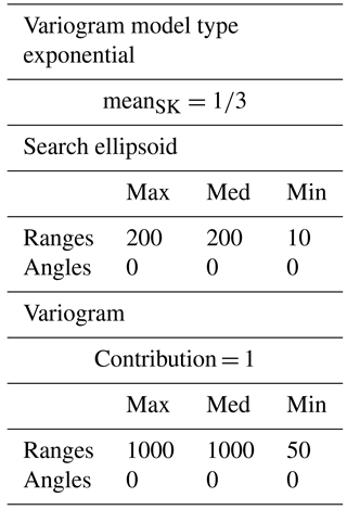
Table A2General SGeMS parameters used for the snesim realizations.
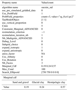
The main author, AASB, developed the concepts and ideas for the paper during a 6-month sabbatical at Stanford University and was the main contributor in regards to writing and compiling the paper. IM helped refine and develop the concepts presented in the paper and aided in the writing process with iterative internal paper reviews. Co-author TNV provided valuable insights into MPS modeling and helped with the practical process of MPS modeling, as well as internal co-author reviews. Co-author FJ helped to guide the research topics that are addressed in this paper. The remaining co-authors, AVC, ASH, and JS, all aided in the co-author review process and contributed with ideas and insights.
The authors declare that they have no conflict of interest.
We would like to thank Senior Research Engineer Celine Scheidt of Stanford
University for pointing us in the direction of using Euclidean distance
transforms for comparing MPS realizations. Three anonymous reviewers and the
editor are thanked for valuable comments that improved the clarity of the
manuscript. This study is supported by HyGEM (Integrating geophysics,
geology, and hydrology for improved groundwater and environmental management,
project no. 11-116763). The funding for HyGEM is provided by the Danish
Council for Strategic Research.
Edited by:
Jesús Carrera
Reviewed by: three anonymous referees
Auken, E., Christansen, A. V., Westergaard, J. H., Kirkegaard, C., Foged, N., and Viezzoli, A.: An integrated processing scheme for high-resolution airborne electromagnetic surveys, the SkyTEM system, Explor. Geophys., 40, 184–192, https://doi.org/10.1071/EG08128, 2009.
Barfod, A. A. S., Møller, I., and Christansen, A. V.: Compiling a national resistivity atlas of Denmark based on airborne and ground-based transient electromagnetic data, J. Appl. Geophys., 134, 199–209, https://doi.org/10.1016/j.jappgeo.2016.09.017, 2016.
Barfod, A. A. S., Møller, I., Christiansen, A. V., Høyer, A.-S., Hoffimann, J., Straubhaar, J., and Caers, J.: Hydrostratigraphic modeling using multiple-point statistics and airborne transient electromagnetic methods, Hydrol. Earth Syst. Sci., 22, 3351–3373, https://doi.org/10.5194/hess-22-3351-2018, 2018.
Christensen, N. K., Minsley, B. J., and Christensen, S.: Generation of 3-D hydrostratigraphic zones from dense airborne electromagnetic data to assess groundwater model prediction error, Water Resour. Res., 53, 1019–1038, https://doi.org/10.1002/2016WR019141, 2017.
Chugunova, T. and Hu, L. Y.: Multiple-Point Simulations Constrained by Continuous Auxiliary Data, Math. Geosci., 40, 133–146, https://doi.org/10.1007/s11004-007-9142-4, 2008.
Comunian, A., Renard, P., and Straubhaar, J.: 3D multiple-point statistics simulation using 2D training images, Comput. Geosci., 40, 49–65, https://doi.org/10.1016/j.cageo.2011.07.009, 2012.
Constable, S. C., Parker, R. L., and Constable, C. G.: Occam's inversion: A practical algorithm for generating smooth models from electromagnetic sounding data, Geophysics, 52, 289–300, https://doi.org/10.1190/1.1442303, 1987.
de Iaco, S. and Maggio, S.: Validation techniques for geological patterns simulations based on variogram and multiple-point statistics, Math. Geosci., 43, 483–500, https://doi.org/10.1007/s11004-011-9326-9, 2011.
Ellis, R. G. and Oldenburg, D. W.: Applied geophysical inversion, Geophys. J. Int., 116, 5–11, https://doi.org/10.1111/j.1365-246X.1994.tb02122.x, 1994.
Ferré, T. P. A.: Revisiting the Relationship Between Data, Models, and Decision-Making, Groundwater, 55, 604–614, https://doi.org/10.1111/gwat.12574, 2017.
Feyen, L. and Caers, J.: Quantifying geological uncertainty for flow and transport modeling in multi-modal heterogeneous formations, Adv. Water Resour., 29, 912–929, https://doi.org/10.1016/j.advwatres.2005.08.002, 2006.
Fleckenstein, J. H., Niswonger, R. G., and Fogg, G. E.: River-aquifer interactions, geologic heterogeneity, and low-flow management, Ground Water, 44, 837–852, https://doi.org/10.1111/j.1745-6584.2006.00190.x, 2006.
Fogg, G. E., Noyes, C. D., and Carle, S. F.: Geologically based model of heterogeneous hydraulic conductivity in an alluvial setting, Hydrogeol. J., 6, 131–143, https://doi.org/10.1007/s100400050139, 1998.
Gelhar, L. W.: Stochastic analysis of flow in heterogeneous porous media, in Fundamental of Transport Phenomena in Porous Media, edited by: Bear, J. and Corapcioglu, Y. M., Springer, the Netherlands, 673–717, 1984.
Goovaerts, P.: Geostatistics for Natural Resource Evaluation, 1st ed., edited by: Journel, A. G., Oxford University Press, New York, 1997.
Gunnink, J. L. and Siemon, B.: Applying airborne electromagnetics in 3D stochastic geohydrological modelling for determining groundwater protection, Near Surf. Geophys., 13, 45–60, https://doi.org/10.3997/1873-0604.2014044, 2015.
Hansen, T. M., Vu, L. T., Mosegaard, K., and Cordua, K. S.: Multiple point statistical simulation using uncertain (soft) conditional data, Comput. Geosci., 114, 1–10, https://doi.org/10.1016/j.cageo.2018.01.017, 2018.
He, X., Koch, J., Sonnenborg, T. O., Jørgensen, F., Schamper, C., and Christian Refsgaard, J.: Transition probability-based stochastic geological modeling using airborne geophysical data and borehole data, Water Resour. Res., 50, 3147–3169, https://doi.org/10.1002/2013WR014593, 2014.
He, X. L., Sonnenborg, T. O., Jørgensen, F., and Jensen, H. J.: Modelling a real-world buried valley system with vertical non-stationarity using multiple-point statistics, Hydrogeol. J., 25, 359–370, https://doi.org/10.1007/s10040-016-1486-8, 2016.
Hermans, T., Nguyen, F., and Caers, J.: Uncertainty in training image-based inversion of hydraulic head data constrained to ERT data: Workflow and case study, Water Resour. Res., 51, 5332–5352, https://doi.org/10.1002/2014WR016460, 2015.
Høyer, A.-S., Jørgensen, F., Sandersen, P. B. E., Viezzoli, A., and Møller, I.: 3D geological modelling of a complex buried-valley network delineated from borehole and AEM data, J. Appl. Geophys., 122, 94–102, https://doi.org/10.1016/j.jappgeo.2015.09.004, 2015.
Høyer, A.-S., Vignoli, G., Hansen, T. M., Vu, L. T., Keefer, D. A., and Jørgensen, F.: Multiple-point statistical simulation for hydrogeological models: 3-D training image development and conditioning strategies, Hydrol. Earth Syst. Sci., 21, 6069–6089, https://doi.org/10.5194/hess-21-6069-2017, 2017.
Jørgensen, F. and Sandersen, P. B. E.: Buried and open tunnel valleys in Denmark—erosion beneath multiple ice sheets, Quaternary Sci. Rev., 25, 1339–1363, https://doi.org/10.1016/j.quascirev.2005.11.006, 2006.
Jørgensen, F., Møller, R. R., Sandersen, P. B. E., and Nebel, L.: 3-D geological modelling of the Egebjerg area , Denmark, based on hydrogeophysical data, Geol. Surv. Den. Green., 20, 27–30, 2010.
Jørgensen, F., Møller, R. R., Nebel, L., Jensen, N. P., Christansen, A. V., and Sandersen, P. B. E.: A method for cognitive 3D geological voxel modelling of AEM data, B. Eng. Geol. Environ., 72, 421–432, https://doi.org/10.1007/s10064-013-0487-2, 2013.
Journel, A. G.: Combining Knowledge From Diverse Sources: An Alternative to Traditional Data, Math. Geol., 34, 573–596, 2002.
Journel, A. G. and Zhang, T.: The Necessity of a Multiple-Point Prior Model, Math. Geol., 38, 591–610, https://doi.org/10.1007/s11004-006-9031-2, 2007.
Krishnan, S.: Combining individual data information: A review and the tau model, Stanford Center for Reservoir Forecasting (SCRF) annual report 17, 1–54, 2004.
LaBolle, E. M. and Fogg, G. E.: Role of Molecular Diffusion in Contaminant Migration and Recovery in an Alluvial Aquifer System, Transport Porous Med., 42, 155–179, https://doi.org/10.1023/A:1006772716244, 2001.
Le Coz, M., Genthon, P., and Adler, P. M.: Multiple-Point Statistics for Modeling Facies Heterogeneities in a Porous Medium: The Komadugu-Yobe Alluvium, Lake Chad Basin, Math. Geosci., 43, 861–878, https://doi.org/10.1007/s11004-011-9353-6, 2011.
Lochbühler, T., Pirot, G., Straubhaar, J., and Linde, N.: Conditioning of Multiple-Point Statistics Facies Simulations to Tomographic Images, Math. Geosci., 46, 625–645, https://doi.org/10.1007/s11004-013-9484-z, 2014.
Lowe, D. G.: Distinctive Image Features from Scale-Invariant Keypoints, Int. J. Comput. Vision, 60, 91–110, https://doi.org/10.1023/B:VISI.0000029664.99615.94, 2004.
Mariethoz, G. and Renard, P.: Reconstruction of Incomplete Data Sets or Images Using Direct Sampling, Math. Geosci., 42, 245–268, https://doi.org/10.1007/s11004-010-9270-0, 2010.
Marker, P. A., Vilhelmsen, T. N., Foged, N., Wernberg, T., Auken, E., and Bauer-Gottwein, P.: Probabilistic predictions using a groundwater model informed with airborne EM data, Adv. Water Resour., 103, 86–98, https://doi.org/10.1016/j.advwatres.2017.03.002, 2017.
Maurer, C. R., Qi, R., Raghavan, V., and Member, S.: A linear time algorithm for computing exact Euclidean distance transforms of binary images in arbitrary dimensions, IEEE T. Pattern Anal., 25, 265–270, https://doi.org/10.1109/TPAMI.2003.1177156, 2003.
Maxey, G. B.: Hydrostratigraphic units, J. Hydrol., 2, 124–129, 1964.
Okabe, H. and Blunt, M. J.: Prediction of permeability for porous media reconstructed using multiple-point statistics, Phys. Rev. E, 70, 1–2, https://doi.org/10.1103/PhysRevE.70.066135, 2004.
Okabe, H. and Blunt, M. J.: Pore space reconstruction using multiple-point statistics, J. Pet. Sci. Eng., 46, 121–137, https://doi.org/10.1016/j.petrol.2004.08.002, 2005.
Pirot, G.: Using Training Images to Build Model Ensembles with Structural Variability, Groundwater, 55, 656–659, https://doi.org/10.1111/gwat.12556, 2017.
Remy, N., Boucher, A., and Wu, J.: Applied geostatistics with SGeMS: a user's guide, Cambridge University Press, 2014.
Royse, K. R.: Combining numerical and cognitive 3D modelling approaches in order to determine the structure of the Chalk in the London Basin, Comput. Geosci., 36, 500–511, https://doi.org/10.1016/j.cageo.2009.10.001, 2010.
Sandersen, P. B. E., Jørgensen, F., Larsen, N. K., Westergaard, J. H., and Auken, E.: Rapid tunnel-valley formation beneath the receding Late Weichselian ice sheet in Vendsyssel, Denmark, Boreas, 38, 834–851, https://doi.org/10.1111/j.1502-3885.2009.00105.x, 2009.
Seifert, D., Sonnenborg, T. O., Refsgaard, J. C., Højberg, A. L., and Troldborg, L.: Assessment of hydrological model predictive ability given multiple conceptual geological models, Water Resour. Res., 48, 1–16, https://doi.org/10.1029/2011WR011149, 2012.
Sørensen, K. I. and Auken, E.: SkyTEM – a new high-resolution transient electromagnetic system, Explor. Geophys., 35, 191–199, https://doi.org/10.1071/EG04194, 2004.
Strebelle, S.: Conditional Simulation of Complex Geological Structures Using Multiple-Point Statistics, Math. Geol., 34, 1–21, https://doi.org/10.1023/A:1014009426274, 2002.
Strebelle, S. and Journel, A. G.: Reservoir modeling using multiple-point statistics, Proc. SPE Annu. Tech. Conf. Exhib., 11, https://doi.org/10.2523/71324-MS, 2001.
Tahmasebi, P., Hezarkhani, A., and Sahimi, M.: Multiple-point geostatistical modeling based on the cross-correlation functions, Comput. Geosci., 16, 779–797, https://doi.org/10.1007/s10596-012-9287-1, 2012.
Tan, X., Tahmasebi, P., and Caers, J.: Comparing training-image based algorithms using an analysis of distance, Math. Geosci., 46, 149–169, https://doi.org/10.1007/s11004-013-9482-1, 2014.
Tarantola, A. and Valette, B.: Generalized nonlinear inverse problems solved using the least squares criterion, Rev. Geophys., 20, 219–232, https://doi.org/10.1029/RG020i002p00219, 1982.
Tran, T.: Improving variogram reproduction on dense simulation grids, Comput. Geosci., 20, 1161–1168, https://doi.org/10.1016/0098-3004(94)90069-8, 1994.
Viezzoli, A., Christansen, A. V., Auken, E., and Sørensen, K. I.: Quasi-3D modeling of airborne TEM data by spatially constrained inversion, Soundings, 73, F1015–F113, https://doi.org/10.1190/1.2895521, 2008.
Vignoli, G., Fiandaca, G., Christansen, A. V., Kirkegaard, C., and Auken, E.: Sharp spatially constrained inversion with applications to transient electromagnetic data, Geophys. Prospect., 63, 243–255, https://doi.org/10.1111/1365-2478.12185, 2015.
Wang, L., Zhang, Y., and Feng, J.: On the Euclidean distance of images, IEEE T. Pattern Anal., 27, 1334–1339, https://doi.org/10.1109/TPAMI.2005.165, 2005.
Xiaofeng, F. and Wei, W.: Centralized binary patterns embedded with image euclidean distance for facial expression recognition, Proc. – 4th Int. Conf. Nat. Comput. ICNC 2008, 4, 115–119, https://doi.org/10.1109/ICNC.2008.94, 2008.
Zhao, Z. and Illman, W. A.: On the importance of geological data for three-dimensional steady-state hydraulic tomography analysis at a highly heterogeneous aquifer-aquitard system, J. Hydrol., 544, 640–657, https://doi.org/10.1016/j.jhydrol.2016.12.004, 2017.