the Creative Commons Attribution 4.0 License.
the Creative Commons Attribution 4.0 License.
 | 19 Oct 2018
Analysis of the streamflow extremes and long-term water balance in the Liguria region of Italy using a cloud-permitting grid spacing reanalysis dataset
Francesco Silvestro
Antonio Parodi
Lorenzo Campo
Luca Ferraris
The characterization of the hydro-meteorological extremes, in terms of both rainfall and streamflow, and the estimation of long-term water balance indicators are essential issues for flood alert and water management services. In recent years, simulations carried out with meteorological models are becoming available at increasing spatial and temporal resolutions (both historical reanalysis and near-real-time hindcast studies); thus, these meteorological datasets can be used as input for distributed hydrological models to drive a long-period hydrological reanalysis. In this work we adopted a high-resolution (4 km spaced grid, 3-hourly) meteorological reanalysis dataset that covers Europe as a whole for the period between 1979 and 2008. This reanalysis dataset was used together with a rainfall downscaling algorithm and a rainfall bias correction (BC) technique in order to feed a continuous and distributed hydrological model. The resulting modeling chain allowed us to produce long time series of distributed hydrological variables for the Liguria region (northwestern Italy), which has been impacted by severe hydro-meteorological events.
The available rain gauges were compared with the rainfall estimated by the dataset and then used to perform a bias correction in order to match the observed climatology. An analysis of the annual maxima discharges derived by simulated streamflow time series was carried out by comparing the latter with the observations (where available) or a regional statistical analysis (elsewhere). Eventually, an investigation of the long-term water balance was performed by comparing simulated runoff ratios (RRs) with the available observations.
The study highlights the limits and the potential of the considered methodological approach in order to undertake a hydrological analysis in study areas mainly featured by small basins, thus allowing us to overcome the limits of observations which refer to specific locations and in some cases are not fully reliable.
- Article
(8873 KB) - Full-text XML
-
Supplement
(61 KB) - BibTeX
- EndNote


The estimation of the magnitude and the probability of occurrence of a certain streamflow is an important task for a number of purposes: risk assessment, design of structural protections against flooding, civil protection and early warning.
The standard approach based on the use of streamflow observations to carry out a statistical analysis on a specific outlet (Kottegoda and Rosso, 1997) is not always possible because of the lack of measurements: this problem can be tackled by means of a frequency regionalization approach (De Michele and Rosso, 2002) exploiting both observed and modeled streamflow (Boni et al., 2007).
On the other hand, studies and methodologies regarding the management of water resources and droughts also have an important role, especially in the perspective of possible future changes in climate and water needs (Calanca et al., 2006; Fu et al., 2007; Döll and Müller, 2012; Asadieh and Krakauer, 2017). In this case, the analysis of long-term water balance components is of primary importance and the evaluation of total runoff and evapotranspiration becomes crucial.
In the last decades, the use of meteorological reanalyses to study basin behavior in different hydrological regimes has become quite frequent, due to the increased reliability and spatiotemporal resolution of numerical weather prediction (NWP) models. Among many others, Choi et al. (2009) investigated the feasibility of temperature and precipitation data of the North American Regional Reanalysis (NARR, about 32 km grid spacing) for hydrological modeling in northern Manitoba watersheds, while Bastola and Misra (2014) showed that reanalysis products outperformed four other meteorological datasets when used as a large-scale precipitation proxy for hydrological response simulations.
Furthermore, Krogh et al. (2015) used the ECMWF interim reanalysis (ERA-Interim, about 70 km grid spacing) as input to model the hydrological response of one of the largest rivers in Patagonia; similarly, Nkiaka et al. (2017) investigated the potential of using global reanalysis datasets in the data-scarce Sudan–Sahel region.
The CORDEX (Coordinated Regional Climate Downscaling Experiment, Giorgi et al., 2009) initiative aims to produce regional climate change projections worldwide to be fed into impact, adaptation and disaster risk reduction studies using fine-scale regional climate models (RCMs) forced by different global climate models (GCMs) of the CMIP5 (Coupled Model Intercomparison Project Phase 5, CMIP5) archive. Along these lines, Kotlarski et al. (2014) confirmed, with simulations on grid resolutions up to about 12 km (0.11∘), the capability of RCMs to correctly reproduce the main features of the European climate for the period 1979–2008. However, they also exhibit relevant modeling errors concerning some metrics, certain regions and seasons: as an example, precipitation biases are in the ±40 % range while seasonally and regionally averaged temperature biases are generally smaller than 1.5 ∘C. Building on these findings, Pieri et al. (2015) moved one step further, in the framework of the EXtreme PREcipitation and Hydrological Climate Scenario Simulations (EXPRESS-Hydro) project, by dynamically downscaling at a finer spatiotemporal resolution (4 km, 3-hourly) the ERA-Interim dataset using the state-of-the-art non-hydrostatic Weather Research and Forecasting (WRF) regional climate model.
In this work the high-resolution (Δt=3 h, Δx=4 km) EXPRESS-Hydro regional dynamical downscaling of historical climate scenarios is used as input to a hydro-meteorological chain including a rainfall downscaling algorithm (Rainfall Filtered Autoregressive Model, RainFARM; Rebora et al., 2006a, b) and a continuous distributed hydrological model (Continuum, Silvestro et al., 2013). As a result, a 30-year-long high-resolution (Δt=1 h, Δx=<500 m) hydrological dataset (e.g., Streamflow and Evapotranspiration) was generated for a reference Mediterranean region. It is noteworthy to highlight that both the Continuum model and RainFARM downscaling algorithm have been already widely employed and tested in the very same study area (Gabellani et al., 2008; Silvestro et al., 2014; Laiolo et al., 2014; Davolio et al., 2017).
The distributed nature of the variables allowed us to investigate the possibility of using the hydrological modeling chain for extreme streamflow statistical analysis (e.g., distribution of annual discharge maxima, ADM) and long-term water balance (e.g., long-term runoff ratio, RR) with a fully distributed approach. Furthermore, the fine spatiotemporal resolution of the forcings, together with the use of a rainfall downscaling model, allowed us to evaluate such a high-resolution reanalysis in regions featured with small hydrological watersheds (Silvestro et al., 2011), complex topography and frequent flash floods (Altinbilek et al., 1997; Cassola et al., 2016). The aforementioned elements, together with the analysis of the distribution of flood extremes, are the main novel contributions of the presented analysis with respect to other works that employ a similar modeling cascade: it is in fact mandatory to use a high-resolution reanalysis since coarser ones cannot reproduce the small-scale rainfall structures that usually trigger such local hydro-meteorological processes (Buzzi et al., 2014; Marta-Almeida, 2016; Pontoppidan et al., 2017; Schwitalla et al., 2017).
The study shows the capabilities and the limits of the considered modeling chain to reproduce low-frequency streamflow and long-term water balance as an alternative to observations in a data-scarce environment or whenever a finer spatial distribution of hydro-meteorological processes is essential.
The paper is organized as follows: Sect. 2 describes the study area, the hydro-meteorological dataset and the models; Sect. 3 shows the results; and in Sect. 4 the discussion and conclusions are reported.

Figure 1Study area geolocation at a large scale (a) and zoomed in (b). Blue lines represent the regional boundaries of Italy, the dashed line shows the main catchments of the study region, red dots represent the meteorological rain gauge stations of the Liguria region of Italy where 32 years (1978–2010) of daily data are available and yellow triangles are the level gauge sections. The digital elevation model highlights the morphology of the region. FR: France, MC: Monte Carlo and IT: Italy.
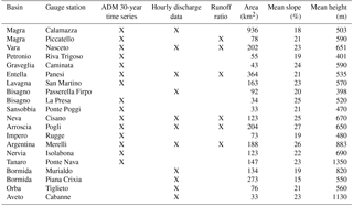
Table 1Availability of discharge data used for model validation, ADM analysis, and long-term mass balance analysis. The characteristics of the basins upstream of each measurement station are reported.
2.1 Study area and case study
The Liguria region is located in northern Italy (Fig. 1) and it is characterized by small- and medium-sized (drainage area in the range 10–1000 km2) and steep-slope (10 %–20 %) basins (Table 1). The response time to precipitation is short, ranging between 0.5 and 10 h (Maidment, 1992; Giannoni et al., 2005). The maximum elevation of mountains is around 2500 m, and most of the region is covered with forest or other types of vegetation like meadows and shrubs; usually the catchments mouths are densely urbanized. The hydrological regime is prevalently torrential and the entire study area is frequently hit by flash floods (Rebora et al., 2013); as a consequence, the variability of annual discharge maxima is high. Winter seasons are generally not very cold, being in a Mediterranean environment but, as the elevation varies from sea level to more than 2000 m, below-zero temperatures are rare (a few days a year) along the coast and at low altitude but they can easily drop even below −10 ∘C inland. Snow occurs only few days a year and normally does not reach the coastal areas.
During warm season peak temperature hardly rises over 31–32 ∘C. The local rain gauge network (OMIRL, Osservatorio Meteo-Idrologico della Regione Liguria) is managed by the Regional Environmental Protection Agency of Liguria (ARPAL) and is quite dense (more than 150 gauges; 1 rain gauge/40 km2 on average), with a 5–10 min resolution and a homogeneous distribution with respect to the elevation. Temperature, radiation, wind and air humidity gauges are also part of the observational network, even though their density is lower, about 1∕50, 1∕200, 1∕200 and 1∕60 km2 respectively. Data from 2011 to 2014 were collected for calibrating–validating the hydrological model.
Besides, for a subset of 95 rain gauge stations (see Fig. 1), ARPAL hosts a web-based free-access validated database of historical (1978–2010) daily precipitation measurements (ARPAL, 2010) that were used in the present study for the bias correction (BC) of the EXPRESS-Hydro reanalysis rainfall estimation.
For 11 level gauge stations seamless hourly data are available from 2011 to 2014 together with rating curves, while annual discharge maxima time series longer than 30 years are available for 15 level gauges (Fig. 1); the latter ones cover sub-periods which are not continuous from 1950 to recent years. Moreover, in the Hydrologic Annual Survey (http://www.arpal.gov.it/homepage/meteo/pubblicazioni/annali-idrologici.html, last access: 12 October 2017), an official document published by ARPAL, annual basin-scale runoff ratios (defined as runoff volume/precipitation) are available for six stations.
In Table 1 the availability of the discharge and discharge-related data is summarized together with hydro-geomorphic characteristics of the basins upstream of each station.
All the data are checked by ARPAL in compliance with WMO recommendations so as to flag errors and unphysical values.
2.2 Bias correction of rainfall fields (BC)
Before being used as input for the hydrological simulations, the EXPRESS-Hydro reanalysis rainfall dataset was compared with the climatological precipitation data of the Liguria rain gauge dataset (ARPAL, 2010). The observational dataset is constituted by validated time series of about 95 rain gauges homogeneously distributed on the Liguria region territory, covering the whole EXPRESS-Hydro dataset (not for all gauges, though) with a daily time step.
In order to provide a hydrological model with the most reliable input data, the EXPRESS-Hydro reanalysis precipitation data were bias corrected with the actual rain gauges so as to assure an accurate reproduction of the local climatology in terms of monthly accumulation. As rainfall was the only available data in the Liguria climatological atlas, the bias correction was not applied to the other variables of the EXPRESS-Hydro dataset.
Nevertheless, several methods are available in the literature to perform a bias correction on different variables (e.g., rainfall, temperature; Fang et al., 2015): among many, in this study a cumulative distribution function (CDF)-matching approach was selected (Fang et al., 2015).
In order to preserve the seasonality and the inter-annual variability, which can be found in the observational data as well as in the EXPRESS-Hydro data, the correction was based on the monthly accumulations computed for both datasets. This led to the generation of 12×N (where N is the number of years of the dataset) maps of monthly cumulated rainfall for EXPRESS-Hydro and 12×Nobs (with Nobs being the number of years of the observed dataset) time series representing the actual cumulated rainfall for each month and for each of the available rain gauges.
To allow for a direct comparison between the observed data and the modeled dataset, the monthly cumulated data from the rain gauges were previously interpolated on the EXPRESS-Hydro spatial grid by using a kriging technique with a spherical variogram. No regression with other spatialized variables (e.g., elevation) was performed because previous tests showed no significant correlation. Due to the high density of the rain gauge network and since the interpolation was applied only to the monthly accumulation, possible errors introduced by the interpolation are assumed to be negligible as short-lived and small-scale rainfall events were addressed (see Boni et al., 2007 and Rebora et al., 2013).
For each cell i, the empirical cumulative distribution functions of both observed and modeled values were computed with the purpose of minimizing the distortions; these CDFs were calculated separately for each month of the year.
In the CDF-matching process the observations CDF was applied to the EXPRESS-Hydro time series of a given cell i in order to obtain the corrected time series of the cumulative monthly rainfall:
where PM is the EXPRESS-Hydro monthly accumulated rainfall, PM′ is the bias-corrected monthly accumulated rainfall, m is the index of the month of the native series, and FMOD,i and FOSS,i are respectively the CDF of the modeled and observed monthly rainfall in the cell i.
Given these corrected monthly time series, the 3 h accumulated rainfall (p in mm) was corrected as follows:
where pi,t is the 3-hourly accumulated rainfall modeled in the cell i at time t, is the bias-corrected 3-hourly accumulated rainfall modeled in the cell i at time t, PMi,m is the monthly accumulated rainfall modeled in the cell i for the month m (in which the instant t falls) and is the monthly accumulated rainfall modeled in the cell i for the month m (in which the time t is) corrected with the CDF-matching approach.
The described procedure allowed us to obtain a 3-hourly maps dataset in which the model bias was eliminated by keeping the characteristics of the modeled output in terms of seasonality and inter-annual variability. Furthermore, the procedure allows us to avoid alterations of possible temporal trends, at both the full-domain and single-cell spatial scale.
The CDF approach allows maintaining the most possible quantity of information furnished by the observations, namely the distribution of the monthly cumulative rainfall; this is not possible with simpler methods (like the simple correction of the average). On the other hand, the temporal structure of the rainfall events at the sub-monthly scale is the one derived from the model, which can bring some kind of distortion with respect to the actual meteorology of the region; the latter constitutes the main limitation of the methodology.
2.3 Downscaling the rainfall with the RainFARM model
RainFARM (Rebora et al., 2006a, b) is a stochastic mathematical model that can be exploited for generating downscaled rainfall fields consistent with the large-scale forecasts provided by either numerical weather prediction systems as in Laiolo et al. (2014) or by expert forecasters (Silvestro and Rebora, 2014). The model takes into account the variability of precipitation at small spatial and temporal scales (e.g., L≤1 km, t≤1 h), preserving the precipitation volume at the scales considered reliable (Lr, and tr) for quantitative precipitation forecasts. In other words Lr and tr are those scales where we expect, on average, a reliable forecast of precipitation volume. RainFARM is able, on the one hand, to preserve spatial and temporal patterns at Lr, tr but, on the other hand, to produce small-scale structures of rainfall which are consistent with detailed remote sensor observations as meteorological-radar estimation (Rebora et al., 2006a).
In the model, the spatiotemporal Fourier spectrum of the precipitation is estimated using the rainfall patterns predicted by a meteorological model and it is mathematically described as follows:
where kx and ky are the x and y spatial wavenumbers, ω is the temporal wavenumber (frequency), and α and β are two parameters that are calibrated fitting the power spectrum of rainfall derived by a NWP system on the frequencies corresponding to the spatiotemporal scales Lr and tr. By extending the spectrum defined by Eq. (3) to the larger wavenumbers (frequencies) it is possible to generate a spatiotemporal rainfall pattern at high resolution (Rebora et al., 2006b). Since the Fourier phases related with the power spectrum (3) are randomly generated before the backwards transformation in real space, RainFARM provides an ensemble of equiprobable high-resolution fields that are consistent with the large-scale precipitation forecasted by a NWP system. RainFARM was designed to feed flood forecasting systems in small- and medium-sized basins (drainage area < 103–104 km2) and it was widely tested on the study area (Rebora et al., 2006a; Silvestro et al., 2012; Silvestro and Rebora, 2014).
In this study the algorithm is used to downscale the bias-corrected EXPRESS-Hydro reanalysis; the nominal grid spacing and temporal resolution of EXPRESS-Hydro precipitation (4 km and 3 h, von Hardenberg et al., 2015 and Pieri et al., 2015) are assumed to be reliable spatial and temporal scales. The downscaling algorithm is not used in probabilistic configuration, but it is instead used to build a possible rainfall spatiotemporal pattern at 1 km and 1 h resolution that is compatible with the runoff at small scales, since most of the catchments in the study area are small sized (often <100–200 km2) with a response time ranging from 1 to 6 h.
2.4 The hydrological model and its calibration–validation
2.4.1 The model: Continuum
The hydrological model used in this study is Continuum (Silvestro et al., 2013), a distributed and continuous model that relies on a space-filling approach and uses a robust way for the identification of the drainage network components (Giannoni et al., 2005). Though all the main hydrological processes are mathematically described in a distributed way, Continuum was designed to be a trade-off between complex physically based models (which describe the physical phenomena with high detail, often introducing complex parameterization) and models with an empirical approach (easy to implement but not accurate enough). The basin or domain of interest is represented through a regular grid, derived by a digital elevation model (DEM), while the flow directions are defined with an algorithm that calculates the maximum slope using the DEM. An algorithm classifies each cell of the drainage network as hillslope or channel flow depending on the main flow regime; a morphologic filter is defined by the expression ASk=C, where A is the drainage area upstream of each cell (L2), S is the local slope (–), and k and C are constants related to the geomorphology of the catchment (Giannoni et al., 2000) – and it is used to determine whether a cell is a hillslope or a channel. The surface flow scheme treats channel and hillslope flows differently: the overland flow (hillslopes) is described by a linear reservoir schematization, while an approach derived by kinematic wave (Wooding, 1965; Todini and Ciarapica, 2001) models the channel flow.
Subsurface flows and infiltration are modeled through an adaptation of the Horton equations (Bauer, 1974; Disikin and Nazimov, 1994) that accounts for soil moisture evolution even in conditions of intermittent and low-intensity rainfall as in Gabellani et al. (2008). Curve number maps are used to estimate some of the subsurface flow parameters (Gabellani et al., 2008).
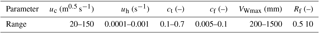
Table 2Ranges of parameter values considered for the calibration–validation process.
Interception of vegetation is schematized with a reservoir that has a retention capacity Sv estimated by static informative layers of vegetation type or leaf area index (LAI) data; the flow in deep soil and the water table evolution are modeled with a distributed linear reservoir schematization and a simplified version of the Darcy equation.
The energy balance uses the force–restore equation (Dickinson, 1988) that allows us to explicitly model the soil surface temperature and to estimate the evapotranspiration from the latent heat flux (Silvestro et al., 2013).
Snow melting and accumulation is simulated with simple equations forced with air temperature and solar radiation (Maidment, 1992) as in Silvestro et al. (2015).
Continuum needs the following input variables: rainfall, air temperature, shortwave incoming solar radiation, wind velocity and relative humidity. When the EXPRESS-Hydro reanalyses are used to feed the model the input variables are 2 m temperature, 10 m wind, rain depth, downward short wave flux at ground surface and 2 m relative humidity.
The parameters that require calibration in the Continuum model are six; they are often estimated at the basin or sub-basin scale: two for the surface flow (uh, m0.5 s−1; and uc, s−1), two for the subsurface flow (ct, –; and cf, –), and two for the deep flow and water table (VWmax, mm; and Rf, –) processes.
The parameter uh affects those hydrograph components which are related to fast surface flow as well as uc but the impact of the latter depends on the length of the channeled paths; cf is related to saturated hydraulic conductivity and controls the subsurface flow rate; ct identifies the part of the water volume in the soil that can be extracted through evapotranspiration only and is thus related to the soil field capacity, while both ct and cf regulate the dynamics of the saturation of the root zone. The two parameters VWmax and Rf control the flow in the deep soil and the dynamic of the water table, yet they impact recession curves and influence flood hydrographs only when large-sized catchments are taken into account (Silvestro et al., 2013).
2.4.2 Implementation on the study area
In the present work, Continuum was implemented with a time resolution of 60 min and a spatial resolution of 0.005∘ (about 480 m). The Shuttle Radar Topography Mission (SRTM) DEM was employed as a terrain model.
Model calibration was performed using observed input and output data without considering reanalysis. This is in the authors' opinion the best approach for several reasons: (i) EXPRESS-Hydro reanalysis data are not involved because they are affected by errors larger than observations ones; (ii) meteorological data at high time resolution are available; (iii) EXPRESS-Hydro reanalysis are too uncertain in terms of geolocation, timing and magnitude of real events – as a consequence streamflow simulations cannot be compared with observations; and (iv) no reliable streamflow data are available for the period covered by the reanalysis.
The model was calibrated on 11 basins where streamflow observations were available at hourly time resolution (see Table 1); the hourly measurements of rainfall, air temperature, solar radiation and air relative humidity provided by the regional weather stations network were interpolated on a 1 km regular grid through a Kriging method to feed the model. The two parameters VWmax and Rf were estimated at the regional scale based also on Davolio et al. (2017), since they are less sensitive than the other four parameters (Silvestro et al., 2013). The observed streamflow data at 60 min time resolution were compared with the model output in order to evaluate its performance. The validation period spanned from 1 January 2013 to 31 December 2014, and the model performance was evaluated through the skill scores, also used in the calibration process (Davolio et al., 2017), as reported in the following.
The Nash–Sutcliffe (NS) coefficient (Nash and Sutcliffe, 1970):
where Qm(t) and Qo(t) are the modeled and observed streamflows at time t. is the mean observed streamflow.
Relative error of high flows (REHF):
where Qth is chosen as the 99th percentile of the observed hydrograph along the calibration period.
While the NS coefficient has the purpose of evaluating the general reproduction of streamflow, the REHF score aims to give more weight to the highest flows, thus leading the calibration to better reproduce the flood events.
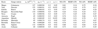
Table 3Hydrological model validation (1 January 2013 to 31 December 2014); skill score values obtained for the calibrated basins with calibrated (CP) and average (AP) parameters. The values of calibrated parameters are also reported. VWmax (mm) and Rf (–) have values of 500 mm and 1 for all the basins.
As in Madsen (2000) the calibration was carried out by combining NS and REHF into a multi-objective function: the space parameter was analyzed using a brute force approach on the time span 2011–2013 in order to optimize the aforementioned multi-objective function. The time resolution of the streamflow data was hourly, while the curve number map was derived by CORINE Land Cover (http://www.sinanet.isprambiente.it/it/progetti/corine-land-cover-1, last access: 10 July 2017). The parameter range values considered during the calibration process were defined considering their physical meaning, the mathematical constraints and the experience – they are reported in Table 2 (Silvestro et al., 2015; Cenci et al., 2016) – the final parameter configuration is similar to the one used in Davolio et al. (2017). Parameter values not involved in calibration are reported in the Appendix.
The values of the skill scores were calculated for the validation period and turned out to be satisfactory, as reported in Table 3.
For those basins where the calibration was not possible, the parameters are assumed to be equal to the average values obtained by the calibration. This assumption was then verified by carrying out a run of the model using the average parameters even for calibrated basins; the statistics maintain good values supporting the significant assumption done. Table 3 reports the skill scores.
Even if the calibration of the model did not encompass all the study region due to the lack of data, the hydrological model (as well) was proven to give good performances as well as similar models specifically developed for the same study area (Giannoni et al., 2000, 2005; Gabellani et al., 2008; Silvestro et al., 2013, 2015; Cenci et al 2016), even in not-calibrated basins (Regione Marche, 2016). In fact, when the basins have similar characteristics, especially regarding the surface response to intense rainfall and the main genesis of the rainfall–runoff process, the parameters often have similar values (Boni et al., 2007).
In order to reduce the warm-up impacts on the 1979 (first year of EXPRESS-Hydro) simulation, a first run was started with a predefined initial condition setup and the state variables simulated on 31 December of every year (from 1979 to 2008) were averaged to estimate a reasonable initial condition for 1 January 1979 to be used in the final simulation.
The hydrological model run for the period 1979–2008 provided a streamflow time series for each pixel of the calculation domain which was, ideally, equivalent to having a gauge every Δx along the hydrological network. Since the spatial resolution of the hydrological model is 480 m, basins smaller than Ath=15 km2 were not taken into account, because the surface water motion processes cannot be modeled with sufficient detail (Giannoni et al., 2005).
2.5 Distribution of the annual discharge maxima
The results of the modeling chain were firstly compared with observations using a typical station-wise comparison approach: 15 gauge stations with at least 30 years of annual discharge maxima (ADM) were identified along the Ligurian territory from east to west.
It was not possible to ensure a perfect overlapping between the simulated and the observational time series; often observed data are not seamless and they may cover longer periods (in some case 50–60 years) with large time spans of missing data (see the table uploaded as additional material). However, on the basis of the conclusions drawn in the Liguria climatological atlas, major climate-change-related trends for the meteorological variables are not evident, thus allowing for the use of the database despite the data gaps.
The comparison between observed and reanalysis-driven ADM is firstly based on the analysis of the respective cumulative density function distributions.
The reanalysis-driven ADM were fitted with a generalized extreme value (GEV) distribution (see e.g., Hosking and Wallis, 1993; Piras et al., 2015) that represents a good compromise between flexibility and robustness. Other works based extreme statistical analysis on the two-components extreme value (TCEV) model (Rossi et al., 1984); nevertheless, we decided to use GEV since it has a smaller number of parameters and it was widely applied (CIMA Research Foundation, 2015; Piras et al., 2015). Moreover, the comparison between the observed and modeled ADM was also done using the Kolmogorov–Smirnov test with a 5 % significance level, in order to verify if they belonged to the same distribution.
2.6 Regional analysis of the annual discharge maxima
In order to carry out a comparison following a distributed approach we referred to Boni et al. (2007), which is one of the operational reference methods in the Liguria region (used by both public authorities and private engineers) to estimate the ADM quantiles (Provincial Authority of Genoa, 2001; Silvestro et al., 2012). The method was conceived and tested especially for the Tyrrhenian catchments of the Liguria region, so the present analysis was carried out only for this area, 45 %–50 % of which is located upstream of the calibrated basins. The method defines a hierarchical approach based on the analysis of the non-dimensional random variable , obtained by grouping together all the available data and making them non-dimensional with respect to each local (gauging station) sample mean, μx, taken as the index flood for gauged sites. Index flood is estimated even where observations were not available by taking advantage of the rainfall regional frequency analysis and rainfall–runoff modeling to allow quantile estimation in each point of the region.
The final result is a methodology to estimate the index flood that can be formalized as follows:
while the quantile is
where T is the return period and K(T) is defined by the non-dimensional regional growth curve, uniquely defined for the whole studied region (Boni et al., 2007).
In the case of the modeling chain analyzed in this work a large number of reanalysis-driven time series are available because a 30-year-long ADM series for each pixel of the model grid can be accessed for basins bigger than Ath. In practice, using a distributed hydrological model, on the one hand, allows the index flood estimation to be a simple mean of a time series in each point of the domain; on the other hand, this provides a large amount of data to build the non-dimensional regional curve.
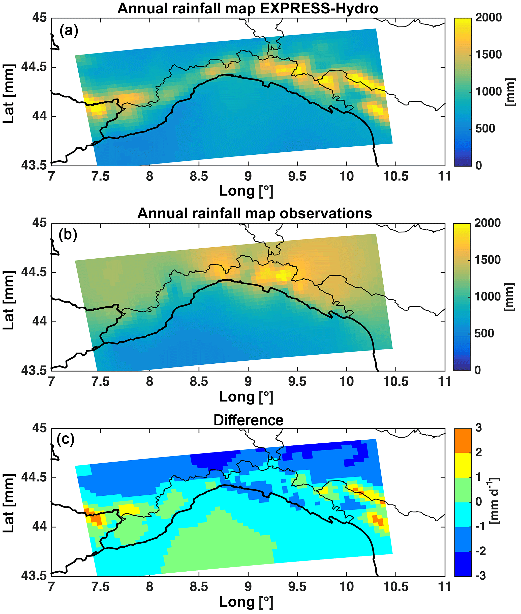
Figure 2(a) shows the average annual rainfall map over the Liguria area, (b) shows the average observed annual rainfall map and (c) shows their difference in mm.
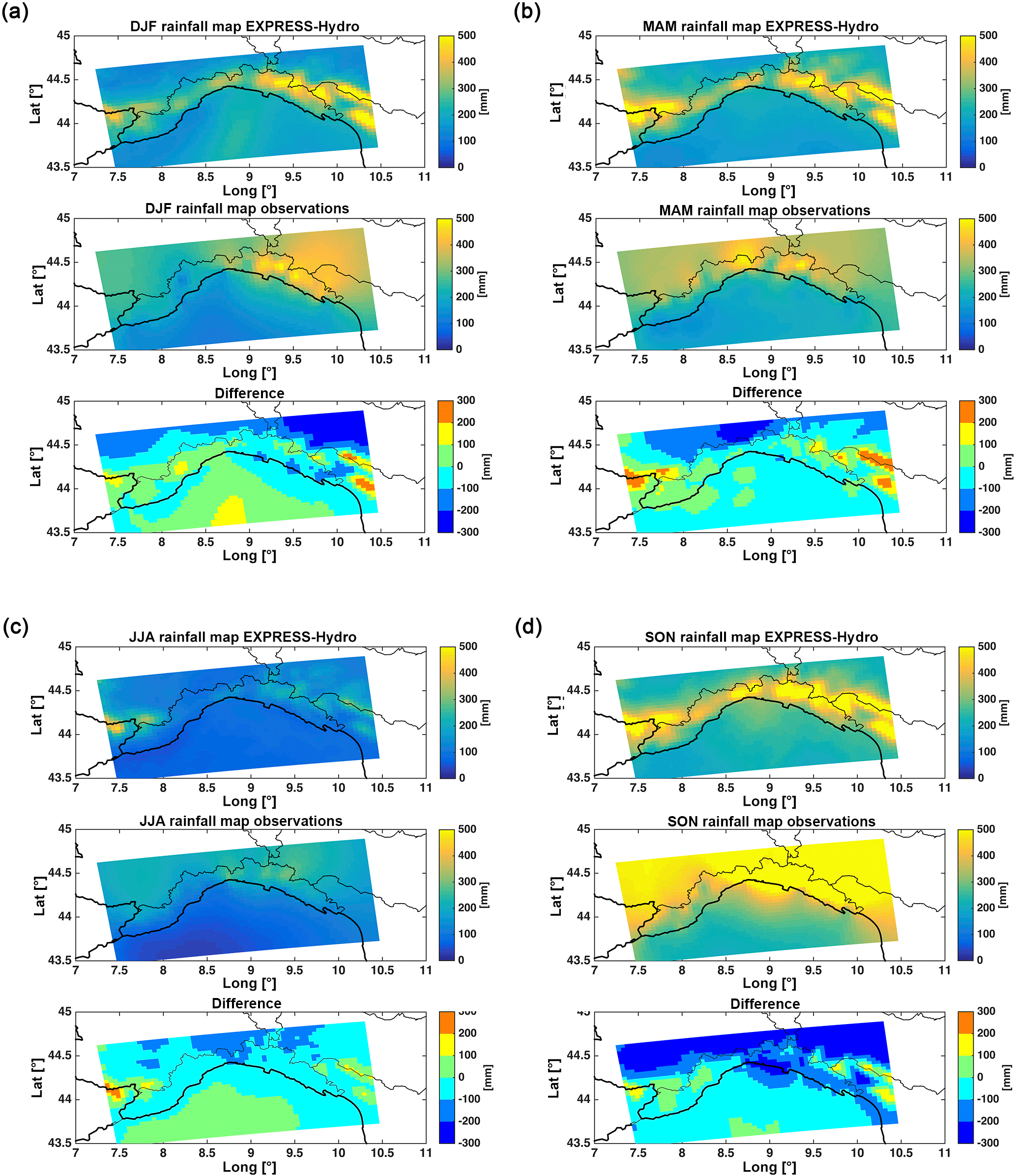
Figure 3The figure shows the average DJF (a), MAM (b), JJA (c) and SON (d) rainfall maps over Liguria. For each season three maps are shown: the EXPRESS-Hydro rainfall map, observed rainfall map and difference map in mm.
3.1 Precipitation analysis
The comparison between EXPRESS-Hydro reanalysis and precipitation climatology over Liguria derived from observational data was undertaken at annual, seasonal, monthly and daily scales.
Pieri et al. (2015), using the EURO4M-APGD reference observational dataset (Isotta et al., 2013, with about 50 daily rain gauge stations in Liguria), already showed an overall underestimation of the WRF rainfall depths on an annual basis, which is more evident on the eastern side of the region (Fig. 3, panels e–f of Pieri et al., 2015), with differences in the range between −2 and −1 mm day−1 on the eastern coastal part and between −1 and 0 mm day−1 on the eastern Apennines side.
The same analysis was repeated and extended in this study, using 95 rain gauges in Liguria: results on annual rainfall depth confirm the findings of Pieri et al. (2015) both on the eastern and western Liguria sides (Fig. 2).
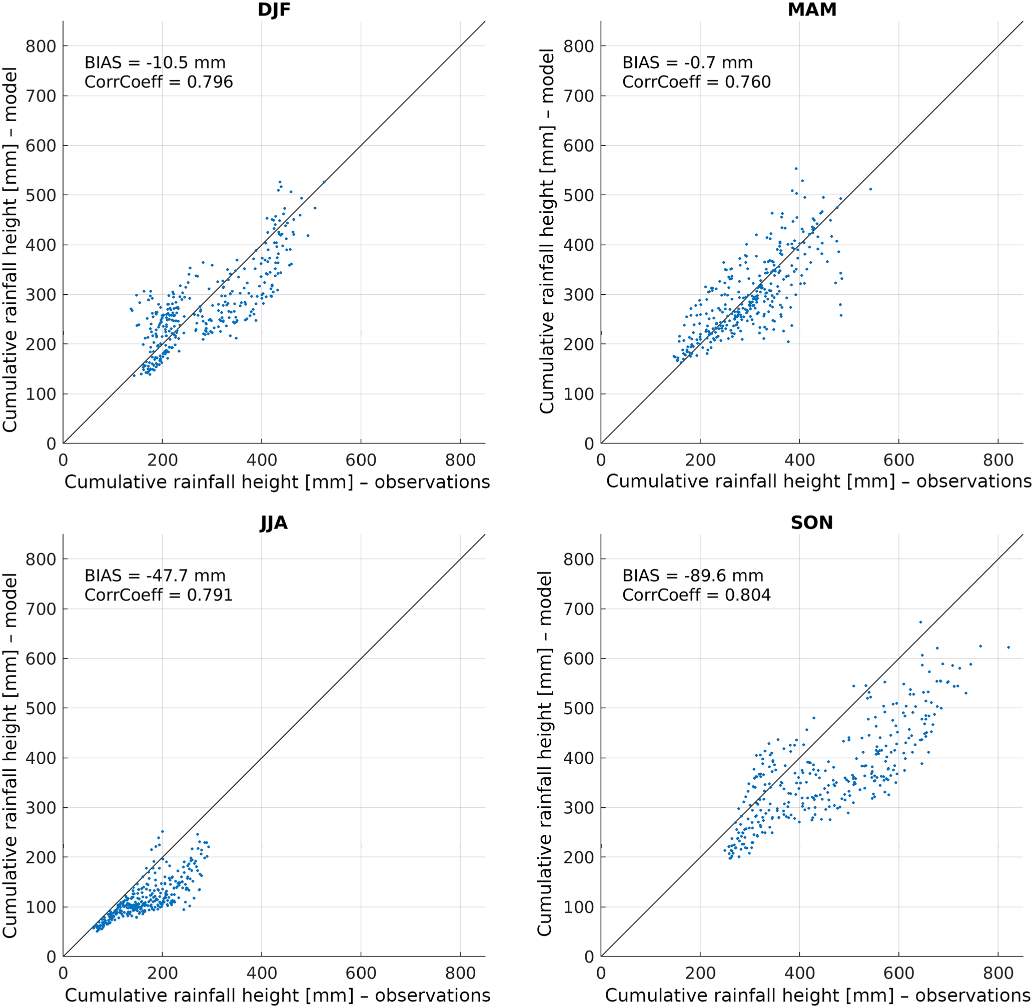
Figure 4Scatter plots of seasonal precipitation built using data on EXPRESS-Hydro spatial resolution (pixel to pixel comparison). The X axis reports observed interpolated rainfall, and the Y axis reports EXPRESS-Hydro estimation.
Table 4Comparison between seasonal rainfall observations and EXPRESS-Hydro. Skill scores estimated on a seasonal timescale.
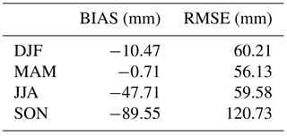
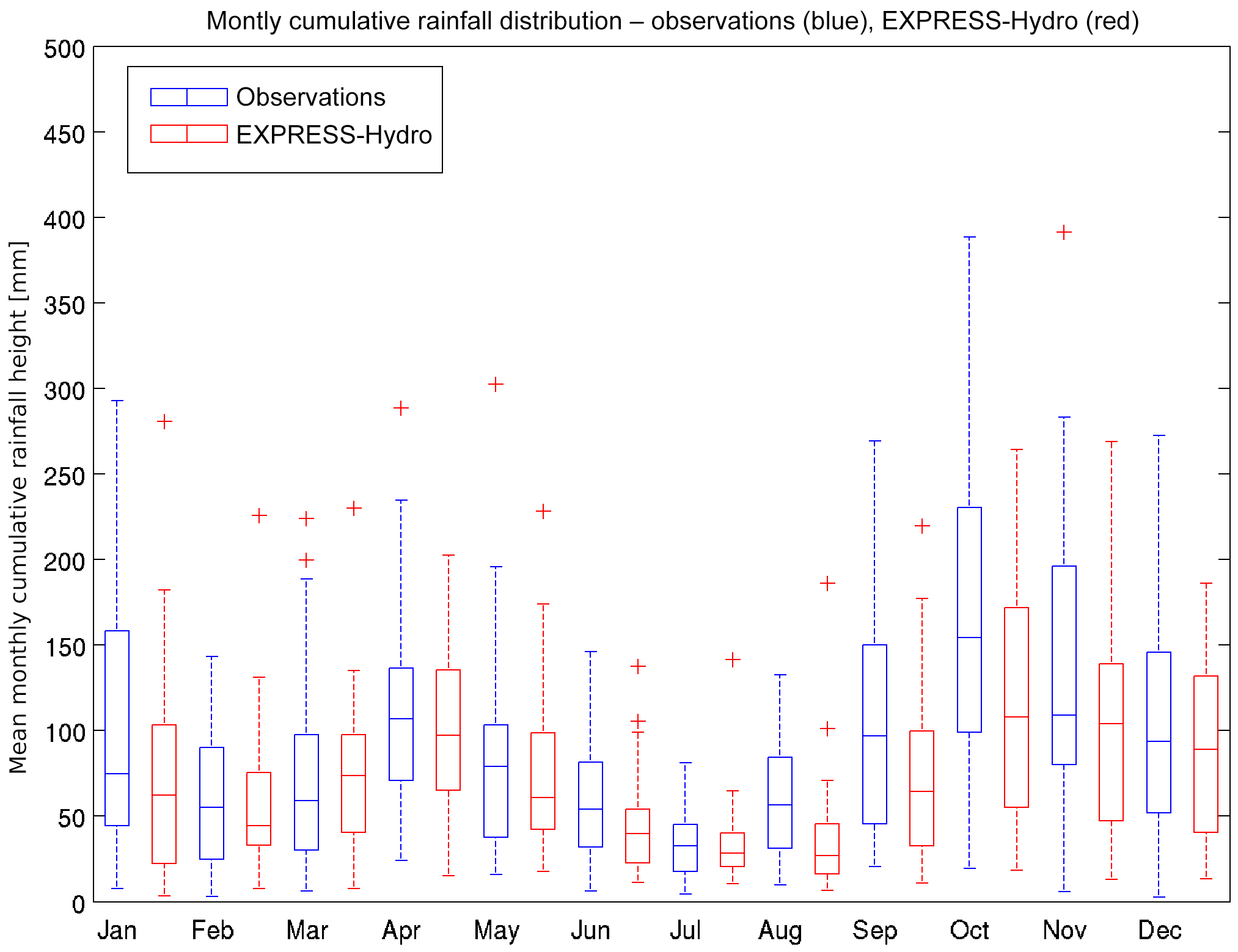
Figure 5Box plot of monthly precipitation averaged at the regional scale. Blue box plots are built with observations while red ones are built with the EXPRESS-Hydro reanalysis.
Concerning the seasonal results, EXPRESS-Hydro tends to underestimate average observed rainfall depths during DJF (Fig. 3) on eastern Liguria (between 0 and 100 mm) while it generally overestimates them on the center-west (0–100 mm); the same holds also for MAM (Fig. 3). During JJA, instead, EXPRESS-Hydro underestimation ranges between 0 and 100 mm over both the western and eastern sides, while it ramps up to 100–200 mm over the center. The underestimation deepens over eastern Liguria during SON (Fig. 3), with values between −100 and 200 mm inland and up to 200–300 mm over the coast. Conversely, on the rest of the region the underestimation drops between 0 and 100 mm. In Fig. 4 the seasonal comparison between observations and EXPRESS-Hydro is also shown in terms of scatter plots, with a good correlation between reanalysis and observations, while in Table 4 we reported the values of the bias and root mean square error (RMSE).
Figure 5 shows the box plot of monthly precipitation averaged at the regional scale for both EXPRESS-Hydro and observations, obtained by averaging the maps of accumulated rainfall. The comparison highlights that EXPRESS-Hydro satisfyingly reproduces the variability along the 30 years, but often underestimates the rainfall amount, particularly in January, September and October.
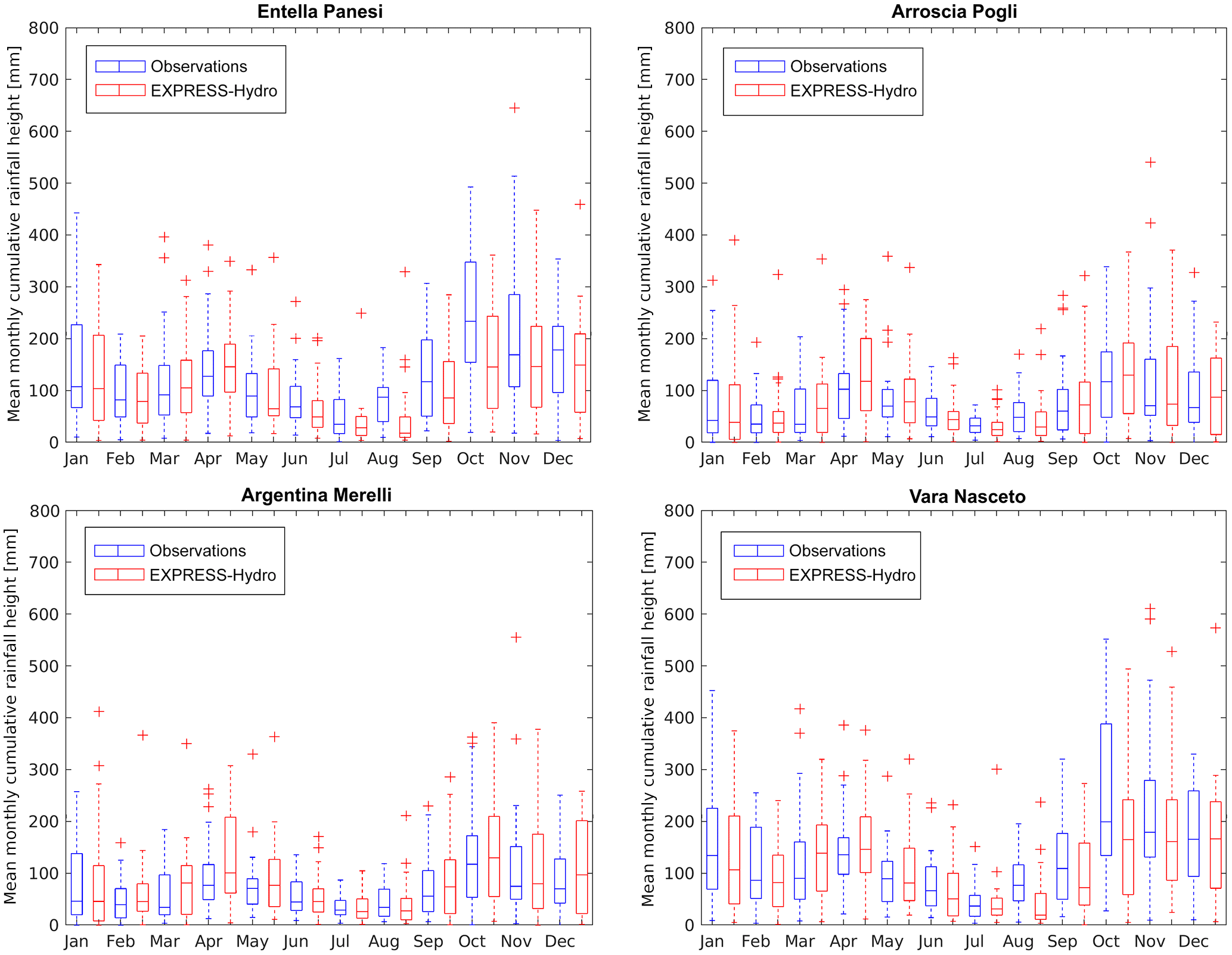
Figure 6Box plot of monthly precipitation averaged at the basin scale for four test catchments. Blue box plots are built with observations while red ones are built with the EXPRESS-Hydro reanalysis.
Figure 6 shows the same analysis of Fig. 5 but at the catchment scale on four basins whose characteristics are reported in Table 1; the basin locations were spread from the east to west side of the region to investigate if different behaviors arise along the study area. It is interesting to note that, while a general underestimation of rainfall during the fall period is found for the rivers located in central-east Liguria (Entella closed at Panesi and Vara closed at Nasceto), the other two test basins behave rather differently as the box plots of Argentina closed at Merelli and Arroscia closed at Pogli show an overestimation during spring, especially in April and May.
A further analysis was carried out in order to understand how EXPRESS-Hydro reanalysis reproduces the rainfall annual maxima, especially after the application of bias correction; ADM of the region are in fact generally driven by very intense rainfall events that have a duration lower than or equal to 24 h. We thus compared the annual maxima of 24 h accumulated rainfall (ARM) derived by observations with those derived by the reanalysis (with BC) again following the approach described in Boni et al. (2007): each series of ARM, observed and modeled, was normalized with its average and a regional non-dimensional distribution function was built. The result is reported in Fig. 7, which shows a very good fit between observations and reanalysis; this confirms a general good reproduction of the climatology even in terms of ARM.

Figure 7Growth curve obtained by annual maxima of 24 h accumulated rainfall. Observations (blue dots) compared with EXPRESS-Hydro reanalysis (black dots). The red line is the GEV distribution fitted on EXPRESS-Hydro values, while dotted lines are the confidence intervals with a 95 % significance.
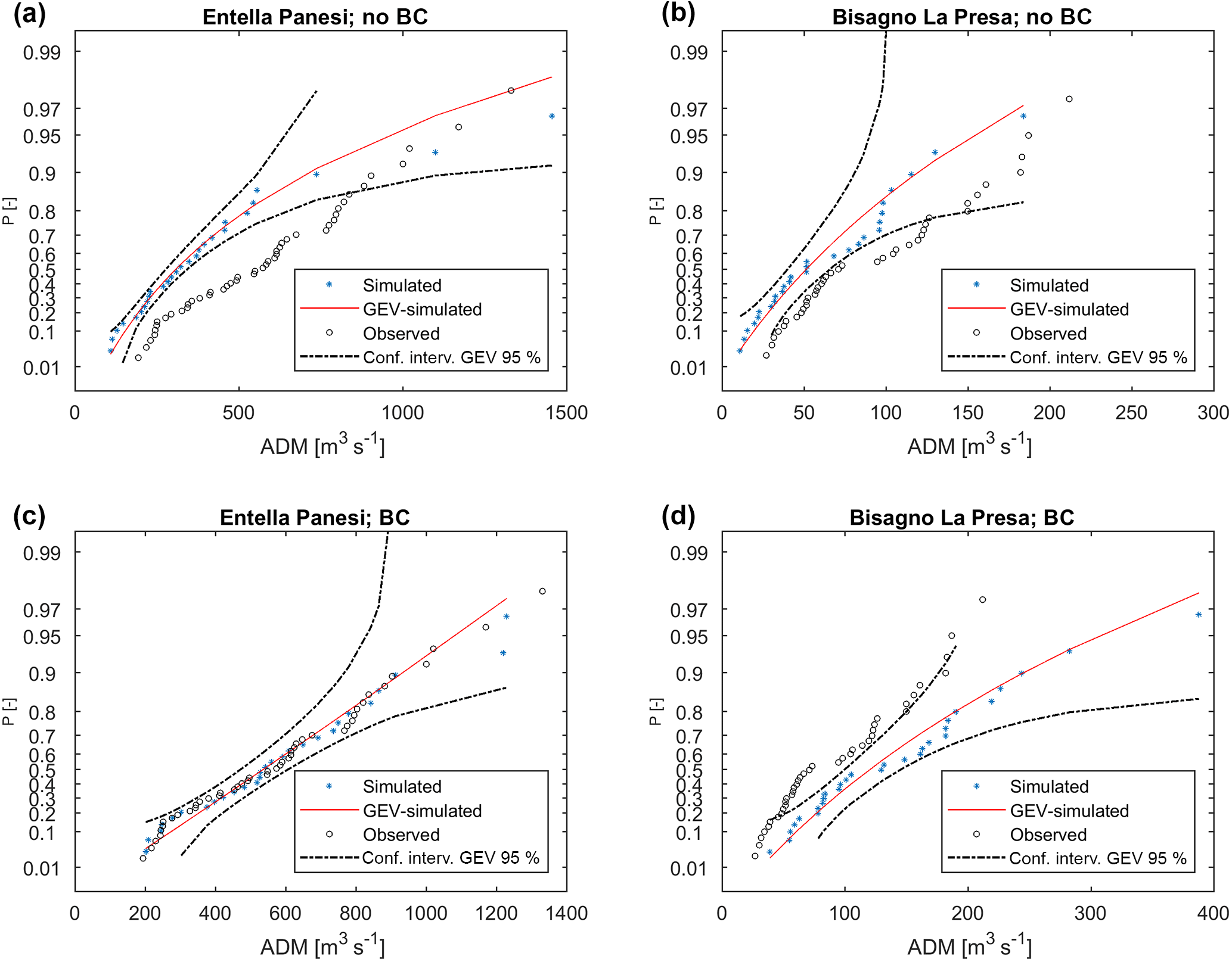
Figure 8Distribution of ADM for Entella closed at Panesi (364 km2) and Bisagno closed at La Presa (34 km2). The blue dots are the simulated ADM, black dots are the observed ADM, red line is the GEV fitted on simulated ADM and dotted lines are the confidence intervals with a 95 % significance. Panels (a) and (b) show results without rainfall bias correction, while (c) and (d) show results with rainfall bias correction.

Figure 9Same as Fig. 8 but for Magra closed at Piccatello (78 km2) and Argentina closed at Merelli (188 km2).
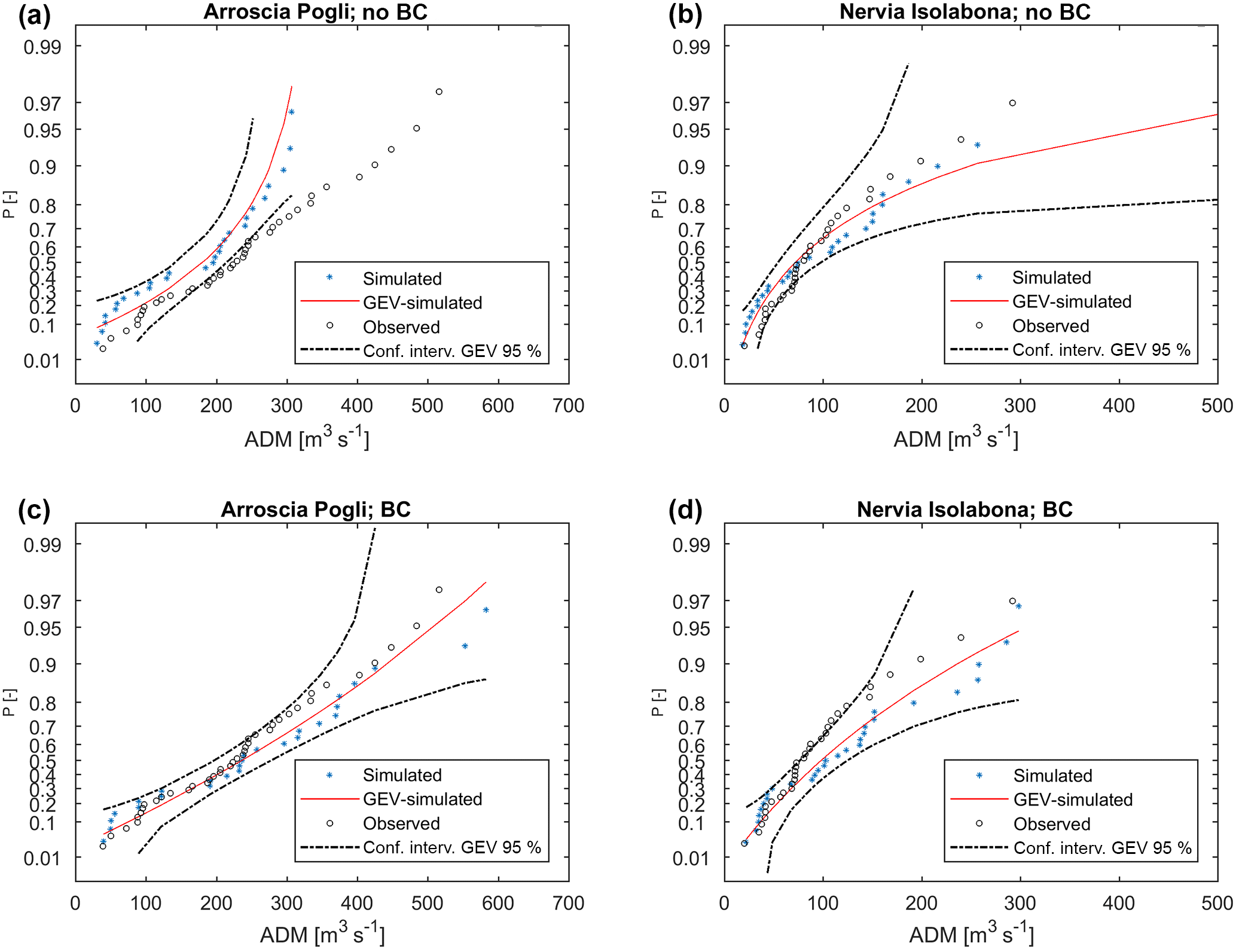
Figure 10Same as Fig. 8 but for Neva closed at Cisano (123 km2) and Nervia closed at Isolabona (122 km2).
3.2 Distribution of the annual discharge maxima
In Figs. 8 to 10 a selection of observed and reanalysis-driven ADM CDF distributions, the GEV and the corresponding 95 % confidence intervals are shown. Six basins were chosen in order to evidence the variability of results, showing either good and poor performances; moreover, the comparisons are referred to hydrological gauging stations where reliable and long-time series of observed ADM are available. For each station the results obtained with and without rainfall BC are both reported.
The cases in Fig. 8 show a shift in the observed distribution with respect to the modeled one, especially without BC. Low ADM observed values lay outside of the confidence intervals of the reanalysis-driven ADM GEV distribution, while the most extreme values fall inside the confidence intervals. The distributions without bias correction show an underestimation of ADM; BC led to very good results for Entella closed at Panesi and to an overestimation for Bisagno closed at La Presa case.
Magra closed at Piccatello (Fig. 9) shows an overestimation in both cases, even higher after the BC; Argentina closed at Merelli benefits from BC, especially regarding the extreme ADM values.
Arroscia closed at Pogli shows an improvement of reanalysis-driven ADM, once BC is performed, while Nervia ADM without BC fits the observations well and BC leads to an overestimation (Fig. 10).
Table 5Kolmogorov–Smirnov (K–S) test with 5 % significance. P values are reported together with verification of the null hypothesis (data can belong to or not belong to the same distribution). Results are reported for the two cases: with (BC) and without (No BC) rainfall bias correction.
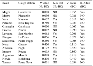
The Kolmogorov–Smirnov test with a 5 % significance level on ADM was applied to all the selected stations and the corresponding results are summarized in Table 5. It is interesting that bias correction does not allow us to increase the number of null hypotheses (data belong to the same distribution), yet 9 stations out of 15 pass the test with either BC applied or not applied. Changing the significance level does not affect the final findings in a significant way: with a 1 % significance, 12 stations pass the test with BC and 11 without BC; with a 10 % significance, 7 stations pass the test with BC and 7 without BC. This fact could derive on how the BC – acting on the monthly volume – affects the short-lived and severe rainfall events that usually are responsible for the ADM in many parts of the study area.
The poor reproduction of ADM in some basins may be due to various causes; on the one hand, it was not possible to calibrate the model over the whole study region, but, on the other hand, in some periods and in some subregions the rainfall reanalysis is probably poorly representative of actual rainfall and BC does not correct it enough. Moreover, observed peaks and simulated peaks often referred to different time periods: this, together with the typical hydro-climatic regime of the study region (flash floods with high variability of ADM) could have a significant impact on final results. There are other sources of uncertainty that can explain the mismatches; the hydrological model can lead to errors (Walker et al., 2003; Liu and Gupta, 2007) due to both its internal structure and to those parameters which are not calibrated but set by literature or by territorial information; furthermore, the input variables are affected by uncertainty, not only rainfall, so they can be causes of errors.
We would like also to highlight the fact that simulated ADM distributions often have similar shapes to the observed ones and suffer a sort of bias (for example Bisagno closed at La Presa, Fig. 8), while in other cases the simulated ADM distribution is only partially out of the confidence intervals (example Argentina closed at Merelli, Fig. 9). The average hydrologic regime on the study region could be only partially affected by the local bad fittings of ADM.
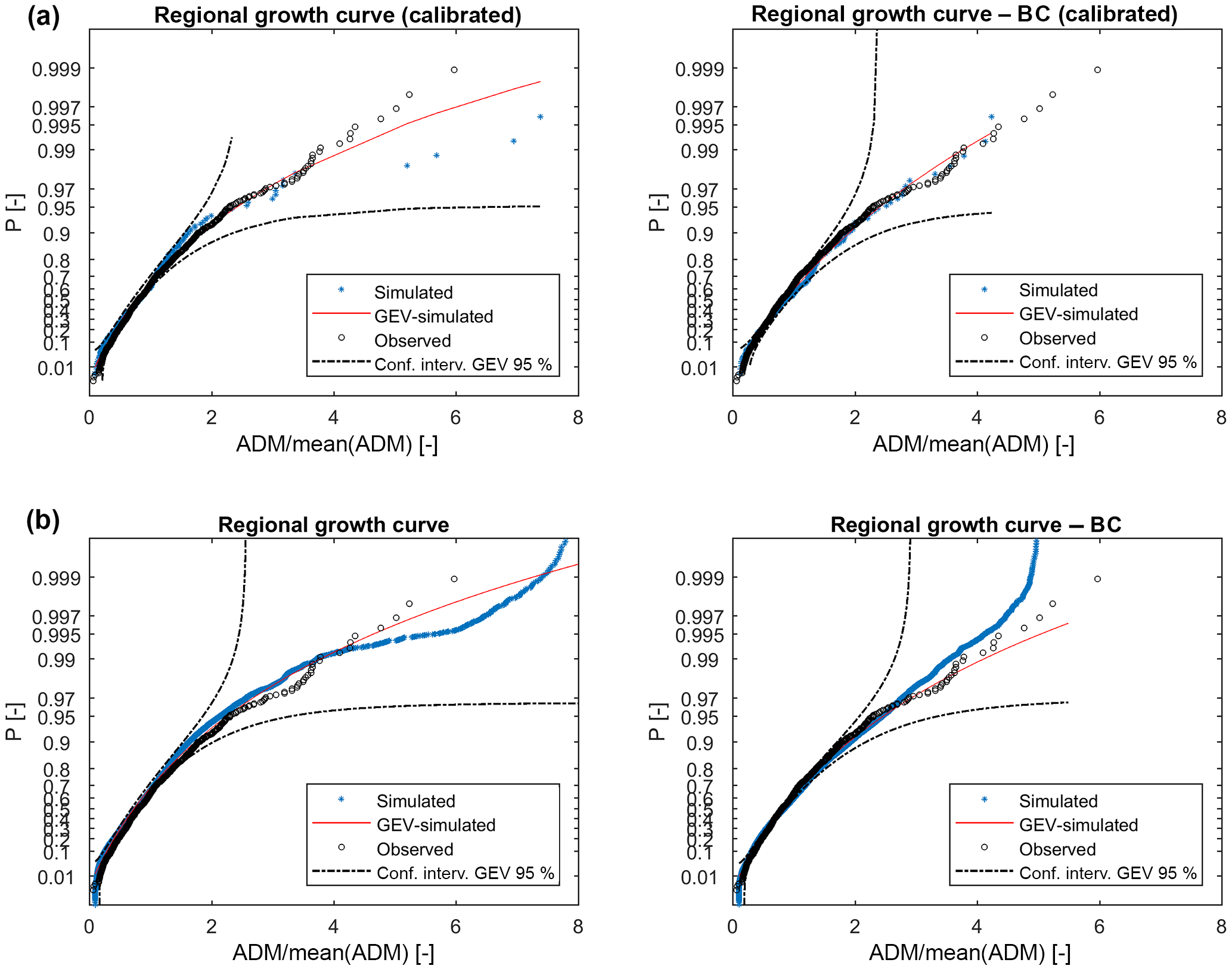
Figure 11Sample growth curve obtained by the model chain (blue dots) compared with observations (black dots). The red line is the GEV distribution fitted on modeled values while dotted lines are the confidence intervals with a 95 % significance. (a) Results without and with rainfall bias correction using the sections where the hydrological model was calibrated. (b) Results without and with rainfall bias correction using all the grid points with drainage area larger than Ath=15 km2.
3.3 Regional analysis of the annual discharge maxima
Figure 11 shows the comparison between the non-dimensional regional growth curve obtained by fitting a GEV on simulated ADM computed with and without BC, the observations (available ADM on the Liguria region) and the simulated ADM. The results are quite good even if it seems that the modeling chain without BC leads to a small underestimation of high-frequency events (low T) and a small overestimation of low-frequency events (high T) with respect to the observations. In any case, both observed and modeled ADM lay inside the confidence intervals (95 %) for a large part of the curve.
In the Fig. 11 we reported the curves built using simulations of all the sub-basins with a drainage area larger than Ath=15 km2 together with those obtained using only the basins where the hydrological model was calibrated. The curves that used only calibrated basins are really similar to the others, proving that the latter configuration enhances the robustness of the regional curve estimation without introducing evident errors.
The main differences in the case of BC configuration are that observations lay always inside the confidence intervals and there is a better matching between simulated and observed sample curves. This is a significant finding; in fact the regional curve is an important ingredient to deal with quantile estimation in ungauged basins. It is important to highlight that the regional approach allows us to reduce the errors that can be found for single basins (Boni et al., 2007) and which are shown in Sect. 3.2; on the one hand, the normalization of each ADM series with its average reduces the effects of bias (due for example to a bad hydrological model calibration and other sources of error), but, on the other hand, the ADM time series of each outlet section (or grid point) is only a small subsample of the entire sample used to build the regional curve. It is in any case important to highlight that good results in terms of the growth curve could be also partially due to the effect of error compensation.
To compare the quantiles estimated using the modeling chain with those in Boni et al. (2007) the following ratio was considered:
where “Model” and “Reg” respectively stand for modeling chain and regional analysis, T is the return period and Q is the ADM. Ideally, if the modeling chain provided exactly the same results of the benchmark regional analysis, the Ratio(T) value should be around 1; Ratio(T) >1 (<1) means overestimation (underestimation).

Figure 12Ratio(T) as a function of drainage area. T=2.9 years, which corresponds to the index flow. (a) shows results without rainfall bias correction and (b) (BC) with rainfall bias correction.
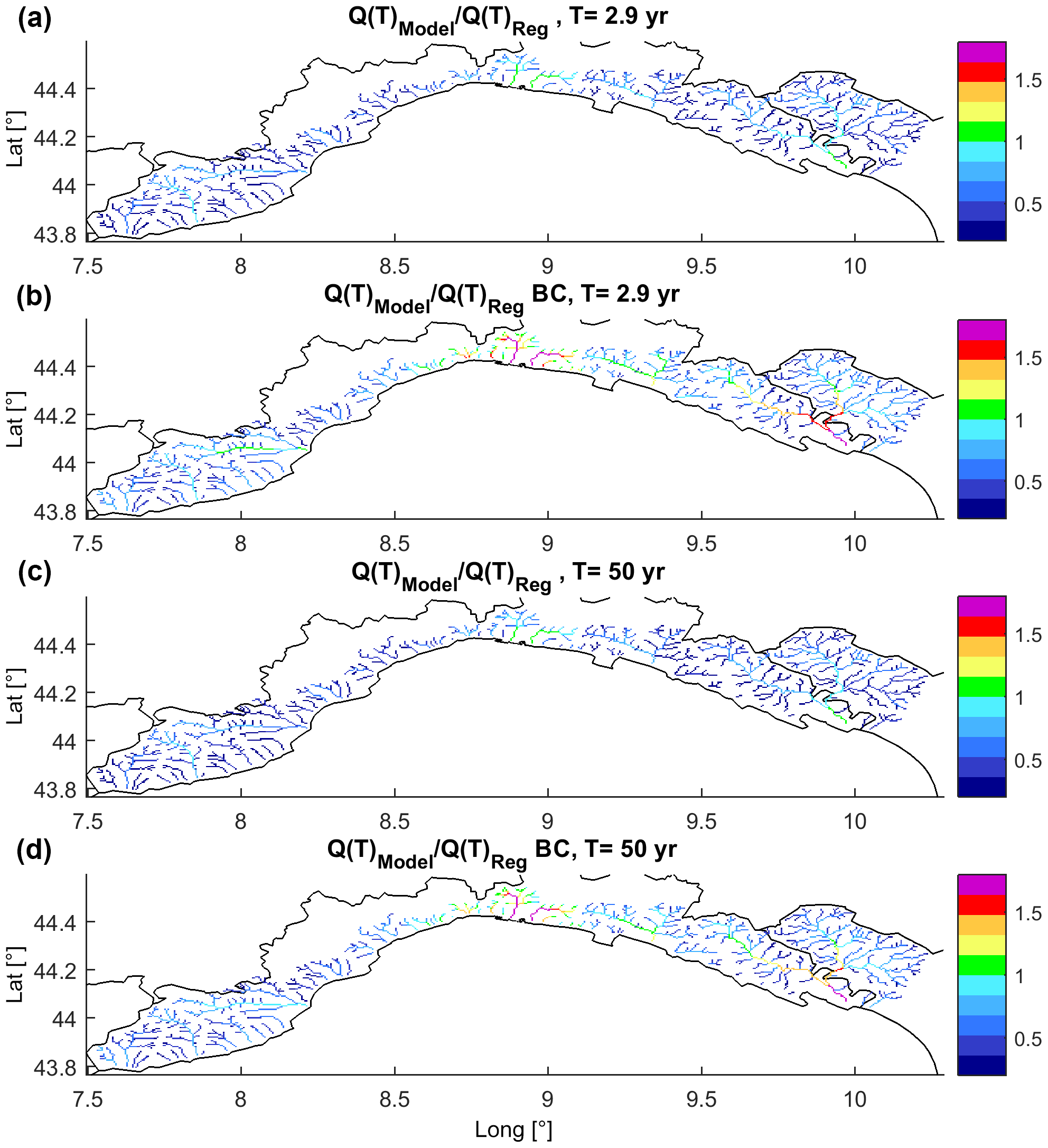
Figure 13Maps of Ratio(T) for T=2.9 and 50 years. (a, b) shows results without rainfall bias correction and (c, d) (BC) with rainfall bias correction. The BC increases the percentage of drainage network points that have values around 1.
Figure 12 shows Ratio(T) for T=2.9 years (index flow) as a function of the drainage area (A in km2), while Fig. 13 shows the maps of Ratio(T) for T=2.9 years and T=50 years.
The first consideration is that a relation between Ratio(T) and A appears to exist even if it is supposedly biased because the size of the sample is biased: the number of small basins is significantly higher than the number of large ones; the chain is not able to reproduce in detail the meteorological and hydrologic processes at very fine temporal and spatial scales (Siccardi et al., 2005) – in fact for A< 30–50 km2 the underestimation seems quite systematic even if BC improves results. Ratio(T) is generally underestimated also for A>30–50 km2, but BC generally leads to a better balance between over- and underestimation. BC enhances overestimation on larger basins (A>200–300 km2). From Fig. 13 a general improvement driven by BC stands out especially in those areas where the model chain without BC underestimates Q(T). Areas where the modeling chain is really close to the benchmark are in green and light blue, whereas dark blue and purple point out where under- or overestimation is high (absolute difference larger than 70–100 %); noticeably, Ratio(T) for T=50 years and T=2.9 years (Fig. 13) have a similar pattern.
In central Liguria the Ratio(T) obtained with EXPRESS-Hydro leads to results comparable with Boni et al. (2007) regardless the use of BC, while simulations with BC are affected by overestimation. This could be due to different causes: (i) EXPRESS-Hydro is likely to well reproduce the events at small temporal and spatial scales (3–6 h, 10–100 km2) in that part of the region as well as generally underestimates monthly accumulation – in this case BC could lead to streamflow overestimation; (ii) the hydrological model may need a better calibration, but it does not seem the most probable option – in fact BC leads to the overestimation of ADM even in calibrated basins, which arose even in the site comparison (Bisagno creek, see Sect. 3.2); (iii) the quantiles in this area may have been underestimated by Boni et al. (2007). It has to be noticed that overestimation is larger for T=2.9 years than for T=50 years (see Fig. 13; some basins are in purple for T=2.9 years and in yellow-orange for T=50 years); this is probably due to the fact that the shape of the growing curve in the BC case leads to a reduction of the overestimation as T increases; the behavior on western Liguria is similar to the center even if less stressed and evident for larger basins only.
The underestimation on smaller catchments (A< 30–50 km2) could be partially due to a non-optimal parameterization of the hydrological model (especially where calibration was not possible), but it appears more reasonable that the errors related to parameterization would lead to a uniform-like distribution between over- and underestimation. However, the model spatial resolution could play a role since the representativeness of the catchment morphology decreases for small drainage areas with a general smoothing effect that affects the results: this degradation effect is clearly continuous from large to small drainage areas, though a threshold for the analysis (i.e., basins with area <16 km2 are neglected) was set.
A further cause is presumably that EXPRESS-Hydro cannot always adequately reproduce the rainfall structures at fine spatial and temporal scales, and the downscaling procedure can only partially correct this drawback. Moreover, the time resolution (1 h after downscaling) could be insufficient when drainage area is small (Silvestro et al., 2016; Rebora et al., 2013); as a consequence, the runoff processes needed to trigger such very small catchments are not properly modeled (Siccardi et al., 2005).
The combination of the aforementioned factors leads us to conclude that the underestimation of quantiles for very small catchments (i.e., A<30–50 km2) is a structural problem of the modeling chain.
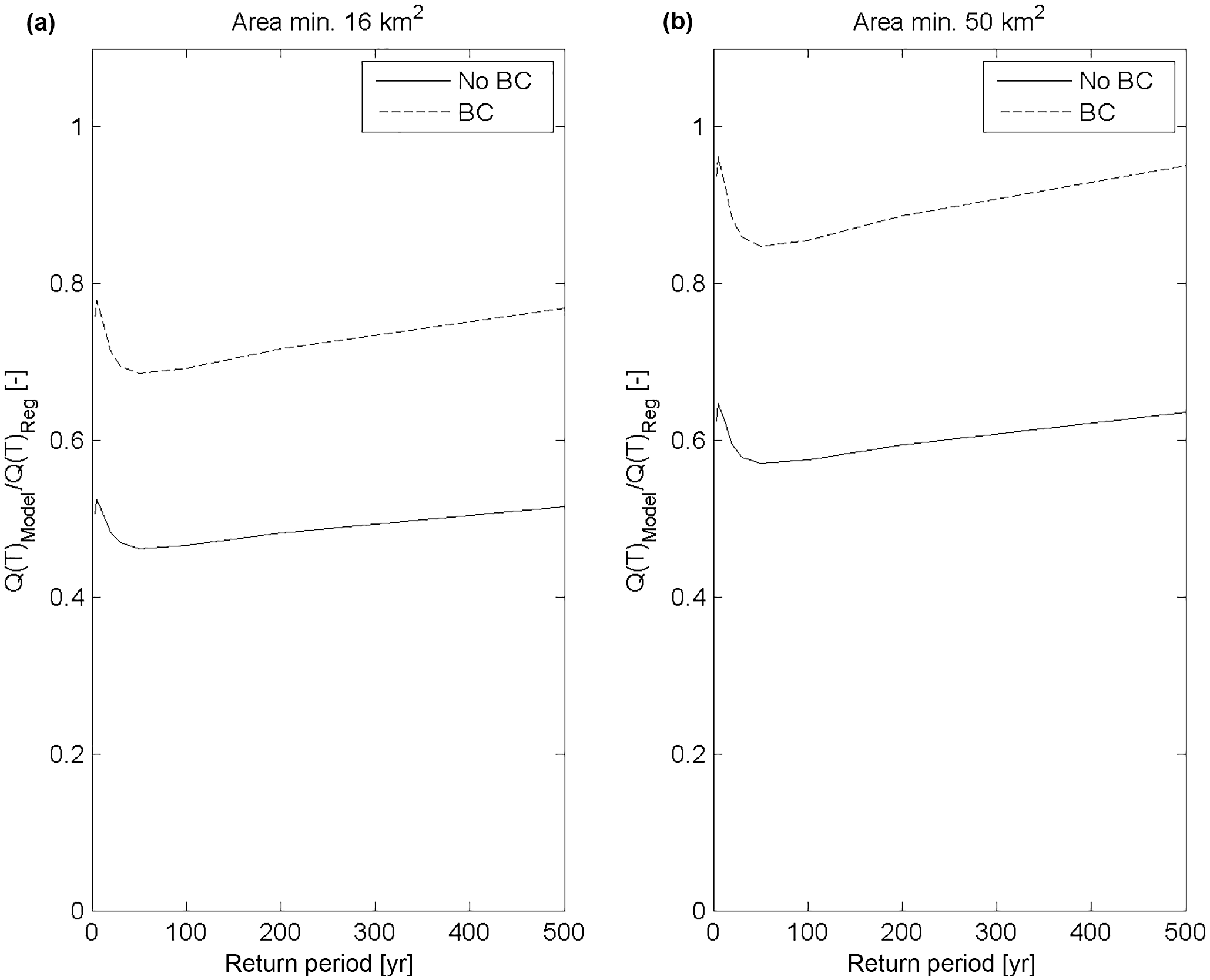
Figure 14Mean Ratio(T) over the considered domain as a function of T. The continuous line (no BC) is the case without rainfall bias correction, and the dotted line (BC) is the case with rainfall bias correction. (a) is the case where points with drainage area lower than 16 km2 are discarded; (b) is the case where points with drainage area lower than 50 km2 are discarded.
This fact is supported by the analysis shown in Fig. 14, left panel. The Ratio(T) averaged on the target area is plotted as a function of T for all the sub-basins with drainage area ≥16 km2. Ratio increases with T especially for the BC case, meaning that the growth curve values K(T) obtained by EXPRESS-Hydro partially balance the underestimation of average ADM (used as index flow) in the estimation of higher quantiles; Ratio(T) for T=2.9 years changes from 0.47 to 0.71 and Ratio(T) for T=50 years from 0.45 to 0.66. If the threshold area is increased from 16 to 50 km2 (Fig. 14, right panel) the underestimation drops for both cases, with and without BC
As already shown, the general underestimation of Ratio(T) for small catchments is not completely confirmed the whole region; for instance, in part of central Liguria results are quite good even for basins with area <50 km2 and bias correction leads to an overestimation of Ratio(T). Apparently, in this area EXPRESS-Hydro can produce rainfall with a spatiotemporal structure able to trigger floods compatible with the hydro-climatology of local small basins. This is also the part of the study region that previous studies demonstrated to be characterized by the highest values of rainfall maxima for 1, 3, 6, 12 and 24 h (Boni et al., 2008).
3.4 Effects of the rainfall downscaling on simulated ADM
In order to assess the influence of the rainfall downscaling, the modeling chain was applied without it. In this way for each pixel of the domain a 30-year-long time series of ADM was computed by the hydrological model driven with the bias-corrected rainfall reanalysis at the EXPRESS-Hydro native resolution. The rainfall field was assumed to have a constant intensity over a 3-hourly time step and resampled from 4 to 1 km.
The 30-year average ADM was computed and compared to the ones obtained by the complete chain by estimating the following ratio for each grid cell:
where QMeanNoDS (QMeanDS) is the average ADM obtained without (with) downscaling. The RatioDS was then plotted versus the drainage area as in Fig. 15: the downscaling impact generally increases as the drainage area decreases, and it is crucial to simulate the ADM on the small catchment when drainage area is lower than 100–150 km2. Moreover, RatioDS is always lower than 1, thus confirming that rainfall downscaling enhances the runoff formation as in Siccardi et al. (2005); likewise, the analysis highlights how the underestimation of quantiles shown in Sect. 3.3 would worsen without it.
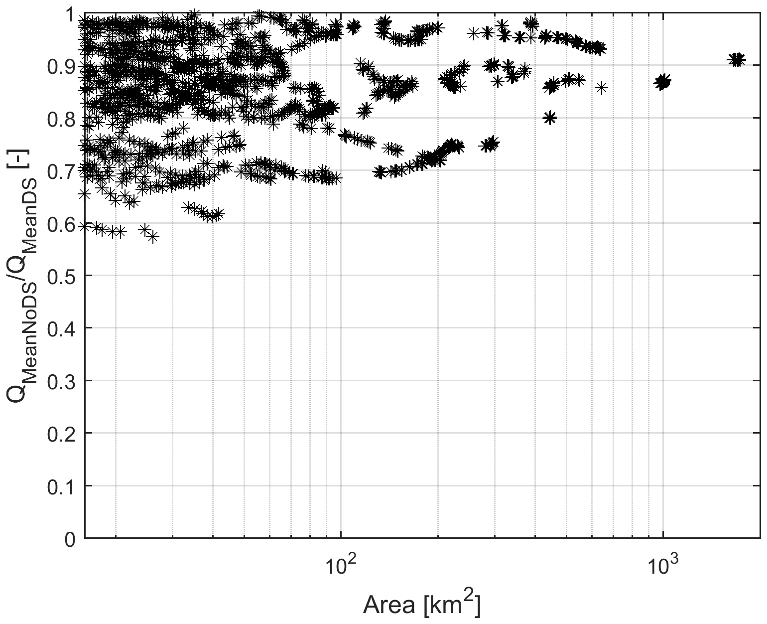
Figure 15Ratio between mean flow estimated without and with downscaling as a function of drainage area. The graph shows that the impact of rainfall downscaling increases when basin drainage area decreases.
3.5 Water balance and runoff ratio
In this section some considerations about the long-term water balance are shown in order to evaluate how the applied system can reproduce the hydrological cycle and the variables related to water balance and water resources management.
Taking advantage of the modeled evapotranspiration maps, the distributed runoff ratio (RR) at the cell scale is estimated as
where Rain(x,y) and Evt(x,y) are the modeled total rainfall and evapotranspiration in the cell with coordinates (x,y) over the 30 years of simulation. The maps of RR are shown in Fig. 16, together with the maps of mean annual rainfall for both cases with and without BC
The spatial pattern of RR is strongly correlated to the precipitation one, and the latter is in turn evidently related with orography, especially for the case without BC
When a single cell has a large number of upstream cells, it tends to be frequently saturated because of the contributions of the subsurface flow of the upstream cells: the values in the cells that belong to the channel network as simulated by the hydrological model (Giannoni et al., 2005) are not shown because they are hardly representative (generally, the values are very low or even negative).

Figure 16Distributed runoff ratio and mean annual rainfall. (a) shows the model estimation without BC while (b) with BC.
BC produces an increase in both the precipitation and runoff ratio on the entire region and a reduction of the differences between coastal and inland areas. In order to estimate how the modeling chain reproduces the available observations the runoff ratio at the basin scale on a target gauge station S is computed by
where Rain(S) is the accumulated rainfall over the basin lying upstream of the gauge station S and VQ(s) is the integral on time of the streamflow volume passed through the gauge station S. We considered some gauge sections where the runoff ratio estimated by observations (rainfall and streamflow) is available (see Table 1) from the Hydrologic Annual Survey (http://www.arpal.gov.it/homepage/meteo/pubblicazioni/annali-idrologici.html, last access: 12 October 2017.), an official document published by the Regional Environmental Protection Agency of Liguria. The observed runoff ratios are not available for the simulation period (1979–2008) but they are estimated as an average of the values measured in non-continuous periods since the 1940s to present, thus providing a possible benchmark to assess the performance of the modeling chain.
Table 6Runoff ratios (RR) obtained by the modeling chain (with and without the rainfall bias correction) compared to those estimated by observations. Results are reported for the two cases: with (BC) and without (No BC) rainfall bias correction.
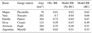
Modeled RRs are compatible with the hydro-climatology of the target area (Barazzuoli and Rigati, 2004; Provincia di Imperia, 2017) but at the same time a general underestimation in the western part of the region is evident (basins Neva, Arroscia, Argentina); BC improves results and RRs are more similar to the benchmark (Table 6).
The rainfall BC introduces only small variations in terms of runoff ratio, thus meaning that when the long-term water balance is addressed the increasing or decreasing of rainfall lead on similar percent variation on both runoff and evapotranspiration.
For example, in the central and eastern parts of Liguria, BC generally increases the precipitation and reduces the orographic features of the spatial pattern, but at the same time the evapotranspiration increases too; consequently, the RRs' rise is small. As shown in Sect. 3.2 and 3.3 the increase in rainfall leads to larger values of ADM, but the RRs do not change significantly; this could be due to the fact that other EXPRESS-Hydro variables that influence the energy balance (and the long-term water balance) like solar radiation or wind speed may benefit from a correction. Nevertheless, no reliable and dense data are available for the entire simulation period. Another approach could be to perform a calibration more focused to preserve long-term runoff. In any case, we could say that generally the results are good and they highlight the potential of using such a modeling chain even for water balance purposes.
This work explores the possibility of using EXPRESS-Hydro, a high-resolution regional dynamical downscaling of the ERA-Interim dataset by means of the state-of-the-art non-hydrostatic Weather Research and Forecasting (WRF) regional climate model for hydrological purposes on small catchments. This was done by feeding a distributed continuous hydrological model with a subset of the EXPRESS-Hydro meteorological variables to produce streamflow simulations; the rainfall fields were downscaled from the native spatiotemporal resolution (4 km, 3 h) to a finer one (1 km, 1 h) before they were used to feed a hydrological model. All the analyses were conducted by either applying or not applying a bias correction to rainfall fields. The study area is Liguria, a region in northwestern Italy, with a particular focus on its Tyrrhenian coast.
Firstly we evaluated the performance of the modeling chain in reproducing extreme streamflow statistics by following two methods: (i) by comparing the statistical distribution of ADM with observations in some gauging points and (ii) by using as a benchmark the regional analysis presented in Boni et al. (2007) that allows a comparison with a distributed approach.
We then evaluated how the modeling chain reproduces the long-term water balance by analyzing the modeled runoff ratios and using as a benchmark the estimations based on observations.
The results are encouraging even if the modeling chain cannot always meet the considered benchmarks with high accuracy. The ADM statistic is quite good in most of the target region but in some subregions the quantiles are sometimes under- or overestimated. Rainfall BC generally improves the underestimation, yet it introduces an overestimation in some basins especially in the central part of the region and in the largest basins.
A single-site comparison of modeled and observed ADM shows that, for a large number of the gauging sites, the time series belong to the same distribution with a 5 % significance; the fitting of modeled ADM with GEV distributions is generally good; and often the observations lay inside the 95 % confidence interval, especially for low-frequency quantiles. It must be noted that, in any case, in some sites the GEV fitting without BC is better than that with BC
A comparison with the regional analysis shows interesting results as the behavior remarkably drifts in some parts of the region, depending on how EXPRESS-Hydro generates the spatiotemporal patterns of precipitation and how much rainfall bias correction is effective.
Both point and distributed analyses show that there is a general underestimation for basins with drainage area smaller than 30–50 km2 but BC is able to tackling it largely. This is probably due to structural problems of the modeling chain under the aforementioned size: for those basins it is necessary to further refine the temporal and spatial scales of the meteorological input (precipitation chiefly, Siccardi at al., 2006; Silvestro et al., 2016), and likely of hydrological model too (Yang et al., 2001). A possible way to deal with very small basins is to better exploit the potential of the downscaling algorithm (RainFARM) that is here used in a deterministic way to generate a possible time (1 h) and space (1 km) pattern with the constraint of maintaining the precipitation volumes and structures generated by EXPRESS-Hydro at its native resolution (3 h, 4 km).
The runoff ratio was used to evaluate long-term water balance. The RR coefficient evaluated on a 30-year-long simulation period at the cell scale reasonably meets the climatology of the region (Barazzuoli and Rigati, 2004; Provincia di Imperia, 2017) and its pattern is highly correlated with annual mean rainfall distribution. RR at the basin scale was compared with observation-based estimates for some gauging points and the values are of the same order of magnitude; however, the modeling chain generally underestimates both configurations even if BC results are slightly better. This could be due to the fact that also the variables related to energy balance (for example the solar radiation and wind) modeled by EXPRESS-Hydro probably need a correction, but this analysis was not carried out, mainly for the lack of reliable and sufficiently dense data.
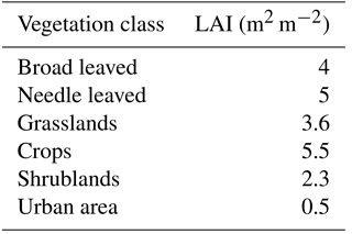
Table 7Vegetation classes and LAI values used to build the LAI map.
To summarize this work, the present modeling chain was proven to reliably simulate the hydro-meteorological statistics in the study area, even if some difficulties and gaps were emphasized by the study. The fully distributed approach allows us to reproduce the hydro-climatic characteristics and features in a seamless way over the whole territory. Rainfall BC, by helping the system to better model some characteristics not completely captured even by a high-resolution meteorological reanalysis, contributes in a relevant way to the improvement of the results even in very small basins (area < 30–50 km2) generally affected by structural underestimation.
The EXPRESS-Hydro data are publicly available via a THREDDS server http://nextdataproject.hpc.cineca.it/thredds/catalog/NextData/eurocdx/h1e4/catalog.html (von Hardenberg, 2017). The different fields are provided in agreement with the CMIP5 data description.
The leaf area index was estimated using a map of vegetation cover (https://geoportal.regione.liguria.it/catalogo/mappe.html, last access: 3 June 2017) and by linking the vegetation types with literature values (Asner et al., 2003) using the classes reported in Table 7. In this application values do not change in time.
In the following we report the values used for those parameters not involved in the calibration, defined in reference to the literature.
Values used to estimate the soil thermal inertia are listed as follows.
-
Soil density: 2700 (kg m−3).
-
Soil specific heat: 733 (J kg−1 K−1).
-
Soil porosity: 0.4 (–).
The values of the neutral component of the bulk heat transfer coefficient were derived by Caparrini et al. (2004) and assigned differently for each season as follows.
-
Winter: (–).
-
Spring: (–).
-
Summer: (–).
-
Autumn: (–).
The supplement related to this article is available online at: https://doi.org/10.5194/hess-22-5403-2018-supplement.
FS and AP has planned, coordinated and collected data needed for this research. All the co-authors contributed to analyzing data and writing and revising the paper.
The authors declare that they have no conflict of interest.
This work is supported by the Italian Civil Protection Department, by
the Regional Environmental Protection Agency of Liguria, Italy (ARPAL), and by the
administration of the Italian region of Liguria. We are grateful to Luca
Molini for his suggestions in reviewing the quality of the
writing.
Edited by: Patricia Saco
Reviewed by: three anonymous referees
Altinbilek, D., Barret, E. C., Oweis, T., Salameh, E., and Siccardi, F.: Rainfall Climatology on the Mediterranean, EU-AVI 080 Project ACROSS – Analyzed climatology rainfall obtained from satellite and surface data in the Mediterranean basin, EC Rep. A VI2-CT93-080, 32 pp., 1997.
ARPAL: Atlante climatico della liguria, available at: http://www.arpal.gov.it/homepage/meteo/analisi-climatologiche/atlante-climatico-della-liguria.html (last access: 12 October 2017), 2010.
Asadieh, B. and Krakauer, N. Y.: Global change in streamflow extremes under climate change over the 21st century, Hydrol. Earth Syst. Sci., 21, 5863–5874, https://doi.org/10.5194/hess-21-5863-2017, 2017.
Asner, G. P., Scurlock, J. M. O., and Hicke, J. A.: Global synthesis of leaf area index observations: implications for ecological and remote sensing studies, Global Ecol. Biogeogr., 12, 191–205, 2003.
Barazzuoli, P. and Rigati, R.: studio per la definizione del bilancio idrogeologico del bacino del fiume Magra, available at: http://www.adbmagra.it/Pdf/UNISI_Bil_Idr_Magra_Rel_Fin.pdf (last access: 2 March 2017) Università degli studi di Siena, 2004.
Bastola, S. and Misra, V.: Evaluation of dynamically downscaled reanalysis precipitation data for hydrological application, Hydrol. Process., 28, 1989–2002, https://doi.org/10.1002/hyp.9734, 2014.
Bauer, S.: A modified Horton equation during intermittent rainfall, Hydrol. Sci. Bull., 19, 219–229, 1974.
Boni, G., Ferraris, L., Giannoni, F., Roth, G., and Rudari, R.: Flood probability analysis for un-gauged watersheds by means of a simple distributed hydrologic model, Adv. Water Resour., 30, 2135–2144, https://doi.org/10.1016/j.advwatres.2006.08.009, 2007.
Boni, G., Parodi, A., and Siccardi, F.: A new parsimonious methodology of mapping the spatial variability of annual maximum rainfall in mountainous environments, J. Hydrometeorol., 9, 492–506, 2008.
Buzzi, A., Davolio, S., Malguzzi, P., Drofa, O., and Mastrangelo, D.: Heavy rainfall episodes over Liguria in autumn 2011: numerical forecasting experiments, Nat. Hazards Earth Syst. Sci., 14, 1325–1340, https://doi.org/10.5194/nhess-14-1325-2014, 2014.
Calanca, P., Roesch, A., Jasper, K., and Wild, M.: Global warming and the summertime evapotranspiration regime of the Alpine region, Clim. Change, 79, 65–78. 2006.
Caparrini, F., Castelli F., and Entekhabi, D.: Estimation of surface turbulent fluxes through assimilation of radiometric surface temperature sequences, J. Hydrometeorol., 5, 145–159, 2004.
Cassola, F., Ferrari, F., Mazzino, A., and Miglietta, M. M.: The role of the sea on the flash floods events over Liguria (northwestern Italy), Geophys. Res. Lett., 43, 3534–3542, 2016.
Cenci, L., Laiolo, P., Gabellani, S., Campo, L., Silvestro, F., Delogu, F., Boni, G., and Rudari, R.: Assimilation of H-SAF Soil Moisture Products for Flash Flood Early Warning Systems, Case Study: Mediterranean Catchments, IEEE J. Sel. Top. Appl., 9, 5634–5646, https://doi.org/10.1109/JSTARS.2016.2598475, 2016.
Choi, W., Kim, S. J., Rasmussen, P. F., and Moore, A. R.: Use of the North American Regional Reanalysis for hydrological modelling in Manitoba, Can. Water Resour. J., 34, 17–36, 2009.
CIMA Foundation: Improvement of the Global Flood model for the GAR 2015, Input Paper prepared for the Global Assessment Report on Disaster Risk Reduction 2015, available at: https://www.unisdr.org/we/inform/publications/49737 (last access: 2 November 2017), 2015.
Davolio, S., Silvestro, F., and Gastaldo, T.: Impact of rainfall assimilation on high-resolution hydro-meteorological forecasts over Liguria (Italy), J. Hydrometeor., 18, 2659–2680, https://doi.org/10.1175/JHM-D-17-0073.1, 2017.
De Michele, C. and Rosso, R.: A multi-level approach to flood frequency regionalisation, Hydrol. Earth Syst. Sci., 6, 185–194, https://doi.org/10.5194/hess-6-185-2002, 2002.
Dickinson, R.: The force-restore method for surface temperature and its generalization, J. Climate, 1, 1086–1097, 1988.
Diskin, M. H. and Nazimov, N.: Linear reservoir with feedback regulated inlet as a model for the infiltration process, J. Hydrol., 172, 313–330, 1994.
Döll, P. and Müller, S.: How is the impact of climate change on river flow regimes related to the impact on mean annual runoff? A global-scale analysi, Environ. Res. Lett., 7, 1–11, 2012.
Fang, G. H., Yang, J., Chen, Y. N., and Zammit, C.: Comparing bias correction methods in downscaling meteorological variables for a hydrologic impact study in an arid area in China, Hydrol. Earth Syst. Sci., 19, 2547–2559, https://doi.org/10.5194/hess-19-2547-2015, 2015.
Fu, G., Charles, S. P., Viney, N. R., Chen, S. L., and Wu, J. Q.: Impacts of climate variability on stream-flow in Yellow River, Hydrol. Process., 21, 3431–3439, 2007.
Gabellani, S., Silvestro, F., Rudari, R., and Boni, G.: General calibration methodology for a combined Horton-SCS infiltration scheme in flash flood modeling, Nat. Hazards Earth Syst. Sci., 8, 1317–1327, https://doi.org/10.5194/nhess-8-1317-2008, 2008.
Giannoni, F., Roth., G., and Rudari, R.: A Semi – Distributed Rainfall – Runoff Model Based on a Geomorphologic Approach, Phys. Chem. Earth, 25, 665–671, 2000.
Giannoni, F., Roth, G., and Rudari, R.: A procedure for drainage network identification from geomorphology and its application to the prediction of the hydrologic response, Adv. Water Resour., 28, 567–581, https://doi.org/10.1016/j.advwatres.2004.11.013, 2005.
Giorgi, F., Jones, C., and Asrar, G. R.: Addressing climate information needs at the regional level: the CORDEX framework, World Meteorological Organization (WMO) Bulletin, 58, 175, 2009.
Hosking, J. R. M. and Wallis, J. R.: Some statistics useful in regional frequency analysis, Water Resour. Res., 29, 271–281, 1993.
Isotta, F. A., Frei, C., Weilguni, V., Percec Tadic, M., Lassègues, P., Rudolf, B., Pavan, V., Cacciamani, C., Antolini, G., Ratto, S. M., Munari, M., Micheletti, S., Bonati, V., Lussana, C., Ronchi, C., Panettieri, E., Marigo, G., and Vertacnik, G.: The climate of daily precipitation in the Alps: Development and analysis of a highresolution grid dataset from pan-Alpine rain-gauge data, Int. J. Climatol., 34, 1657–1675, https://doi.org/10.1002/joc.3794, 2013.
Kotlarski, S., Keuler, K., Christensen, O. B., Colette, A., Déqué, M., Gobiet, A., Goergen, K., Jacob, D., Lüthi, D., van Meijgaard, E., Nikulin, G., Schär, C., Teichmann, C., Vautard, R., Warrach-Sagi, K., and Wulfmeyer, V.: Regional climate modeling on European scales: a joint standard evaluation of the EURO-CORDEX RCM ensemble, Geosci. Model Dev., 7, 1297–1333, https://doi.org/10.5194/gmd-7-1297-2014, 2014.
Kottegoda, N. T. and Rosso, R.: Statistics, Probability, and Reliability for Civil and Environmental Engineers, McGraw-Hill Companies, New York, 1997.
Krogh, S., Pomeroy, J. W., and Mcphee, J. P.: Physically based mountain hydrological modeling using reanalysis data in patagonia, J. Hydrometeorol., 16, 172–193, 2015.
Laiolo, P., Gabellani, S., Rebora, N., Rudari, R., Ferraris, L., Ratto, S., Stevenin, H., and Cauduro, M.: Validation of the Flood-PROOFS probabilistic forecasting system, Hydrol. Process., 28, 3466–3481, https://doi.org/10.1002/hyp.9888, 2014.
Liu, Y. and Gupta, H. V.: Uncertainty in hydrologic modeling: Toward an integrated data assimilation framework, Water Resour. Res., 43, W07401, https://doi.org/10.1029/2006WR005756, 2007.
Madsen, H.: Automatic calibration of a conceptual rainfall–runoff model using multiple objectives, J. Hydrol., 235, 276–288, 2000.
Maidment, D.: Handbook of Hydrology, McGraw-Hill, Inc, New York, 1992.
Marta-Almeida, M., Teixeira, J. C., Carvalho, M. J., Melo-Gonçalves, P., and Rocha, A. M.: High resolution WRF climatic simulations for the Iberian Peninsula: model validation, Phys. Chem. Earth Parts A/B/C, 94, 94–105, 2016.
Nkiaka, E., Nawaz, N. R., and Lovett, J. C.: Evaluating Global Reanalysis Datasets as Input for Hydrological Modelling in the Sudano-Sahel Region, Hydrology, 4, 1–19, 2017.
Nash, J. E. and Sutcliffe, J. V.: River flood forecasting through conceptual models I: a discussion of principles, J. Hydrol., 10, 282–290, 1970.
Pieri, A. B., von Hardenberg, J., Parodi, A., and Provenzale, A.: Sensitivity of Precipitation Statistics to Resolution, Microphysics, and Convective Parameterization: A Case Study with the High-Resolution WRF Climate Model over Europe, J. Hydrometeorol., 16, 1857–1872, 2015.
Piras, M., Mascar, G., Deidda, R., and Vivoni, E. R.: Impacts of climate change on precipitation and discharge extremes through the use of statistical downscaling approaches in a Mediterranean basin, Sci. Total Environ., 543, 952–964, https://doi.org/10.1016/j.scitotenv.2015.06.088, 2015.
Pontoppidan, M., Reuder, J., Mayer, S., and Kolstad, E. W.: Downscaling an intense precipitation event in complex terrain: the importance of high grid resolution, Tellus A, 1271561, https://doi.org/10.1080/16000870.2016.1271561, 2017.
Provincia di Imperia: Piano di bacino stralcio sul bacino idrico del torrente Arroscia, available at: http://pianidibacino.provincia.imperia.it/Portals/_pianidibacino/Documents/Cap _4.pdf, last access: 2 March 2017.
Provincial Authority of Genoa: River basin planning of the Bisagno creek, available at: http://cartogis.provincia.genova.it/cartogis/pdb/bisagno (last access: 4 April 2007), 2001.
Rebora, N., Ferraris, L., von Hardenberg, J., and Provenzale, A.: Rainfall downscaling and flood forecasting: a case study in the Mediterranean area, Nat. Hazards Earth Syst. Sci., 6, 611–619, https://doi.org/10.5194/nhess-6-611-2006, 2006a.
Rebora, N., Ferraris, L., Hardenberg, J. H., and Provenzale, A.: The RainFARM: Rainfall Downscaling by a Filtered Auto Regressive Model, J. Hydrometeorol., 7, 724–738, 2006b.
Rebora, N., Molini, L., Casella, E., Comellas, A., Fiori, E., Pignone, F., Siccardi, F., Silvestro, F., Tanelli, S., and Parodi, A.: Extreme Rainfall in the Mediterranean: What Can We Learn from Observations?, J. Hydrometeorol., 14, 906–922, 2013.
Regione Marche: Regionalizzazione delle portate massime annuali al colmo di piena per la stima dei tempi di ritorno delle grandezze idrologiche, available at: http://www.regione.marche.it/Regione-Utile/Protezione-Civile/Progetti-e-Pubblicazioni/Studi-Meteo-Idro#Studi-Idrologici-e-Idraulici (last access: 19 October 2017), 2016.
Rossi, F., Fiorentino, M., and Versace, P.: Two component extreme value distribution for flood frequency analysis, Water Resour Res., 20, 847–856, 1984.
Schwitalla, T., Bauer, H.-S., Wulfmeyer, V., and Warrach-Sagi, K.: Continuous high-resolution midlatitude-belt simulations for July–August 2013 with WRF, Geosci. Model Dev., 10, 2031–2055, https://doi.org/10.5194/gmd-10-2031-2017, 2017.
Siccardi, F., Boni, G., Ferraris, L., and Rudari, R.: A hydro-meteorological approach for probabilistic flood forecast, J. Geophys. Res, 110, D05101, https://doi.org/10.1029/2004jd005314, 2005.
Silvestro, F. and Rebora, N.: Impact of precipitation forecast uncertainties and initial soil moisture conditions on a probabilistic flood forecasting chain, J. Hydrol., 519, 1052–1067, 2014.
Silvestro, F., Rebora, N., and Ferraris, L.: Quantitative flood forecasting on small and medium size basins: a probabilistic approach for operational purposes, J. Hydrometeorol., 12, 1432–1446, 2011.
Silvestro, F., Gabellani, S., Giannoni, F., Parodi, A., Rebora, N., Rudari, R., and Siccardi, F.: A hydrological analysis of the 4 November 2011 event in Genoa, Nat. Hazards Earth Syst. Sci., 12, 2743–2752, https://doi.org/10.5194/nhess-12-2743-2012, 2012.
Silvestro, F., Gabellani, S., Delogu, F., Rudari, R., and Boni, G.: Exploiting remote sensing land surface temperature in distributed hydrological modelling: the example of the Continuum model, Hydrol. Earth Syst. Sci., 17, 39–62, https://doi.org/10.5194/hess-17-39-2013, 2013.
Silvestro, F., Gabellani, S., Rudari, R., Delogu, F., Laiolo, P., and Boni, G.: Uncertainty reduction and parameter estimation of a distributed hydrological model with ground and remote-sensing data, Hydrol. Earth Syst. Sci., 19, 1727–1751, https://doi.org/10.5194/hess-19-1727-2015, 2015.
Silvestro, F., Rebora, N., Giannoni, F., Cavallo, A., and Ferraris, L.: The flash flood of the Bisagno Creek on 9th October 2014: an “unfortunate” combination of spatial and temporal scales, J. Hydrol., 541, 50–62, https://doi.org/10.1016/j.jhydrol.2015.08.004, 2016.
Todini, E. and Ciarapica, L.: The TOPKAPI model, in: Mathematical models of largewatershed hydrology, edited by: Singh V. P., Chap. 12, Water Resources Publications, Highlands Ranch, 2001.
von Hardenberg, J., Parodi, A., Pieri, A. B., and Provenzale, A.: Impact of Microphysics and Convective Parameterizations on Dynamical Downscaling for the European Domain, in: Engineering Geology for Society and Territory, edited by: Lollino, G., Manconi, A., Clague, J., Shan, W., and Chiarle, M., Springer International Publishing, Vol. 1, 209–213, 2015.
von Hardenberg, J. and Parodi, A.: EXPRESS-Hydro data set, available at: http://nextdataproject.hpc.cineca.it/thredds/catalog/NextData/eurocdx/h1e4/catalog.html, last access: 3 July 2017.
Walker, W. E., Harremoes, P., Rotmans, J., Van der Sluijs, J. P., Van Asselt, M. B. A, Janssen, P., and Krayer von Kraus, M. P.: Defining Uncertainty: A Conceptual Basis for Uncertainty Management in Model-Based Decision Support, Integrated Assessment, https://doi.org/10.1076/iaij.4.1.5.16466, 2003.
Wooding, R. A.: A hydraulic modeling of the catchment-stream problem. 1. Kinematic wave theory, J. Hydrol., 3, 254–267, 1965.
Yang, D., Herath S., and Musiake K.: Spatial resolution sensitivity of catchment geomorphologic properties and the effect on hydrological simulation, Hydrol. Process., 15, 2085–2099, https://doi.org/10.1002/hyp.280, 2001.