the Creative Commons Attribution 4.0 License.
the Creative Commons Attribution 4.0 License.
 | 11 Oct 2018
Numerical modeling of flow and transport in the Bari industrial area by means of rough walled parallel plate and random walk models
Claudia Cherubini
Nicola Pastore
Dimitra Rapti
Concetta I. Giasi
Modeling fluid flow and solute transport dynamics in fractured karst aquifers is one of the most challenging tasks in hydrogeology.
The present study investigates the hotspots of groundwater contamination in the industrial area of Modugno (Bari – southern Italy), where the limestone aquifer has a fractured and karstic nature.
A rough walled parallel plate model coupled with a geostatistical analysis to infer the values of the equivalent aperture has been implemented and calibrated on the basis of piezometric data. Using the random walk theory, the steady-state distribution of hypothetical contamination with the source at the hotspot has been carried out, reproducing a pollution scenario which is compatible with the observed one. From an analysis of the flow and transport pattern it is possible to infer that the anticline affecting the Calcare di Bari formation in direction ENE–WSW influences the direction of flow as well as the propagation of the contaminant.
The results also show that the presence of nonlinear flow influences advection, in that it leads to a delay in solute transport with respect to the linear flow assumption. This is due to the non-constant distribution of solutes according to different pathways for fractured media which is related to the flow rate.
- Article
(7636 KB) - Full-text XML
-
Supplement
(53 KB) - BibTeX
- EndNote


The characterization and the description of phenomena that involve fractured aquifers, especially when considered in relation to water resource exploitation, are important issues because fractured aquifers serve as the primary source of drinking water for many areas of the world. In fractured rock aquifers, groundwater is stored in the fractures, joints, bedding planes, and cavities of the rock mass. The ability of a fracture to transmit water as well as contaminants depends primarily on the size of the opening, or the fracture aperture.
The parallel plate model is widely used to simulate flow in a fracture due to its simplicity in idealizing a fracture. Many researchers (Baker, 1955; Huitt, 1956; Snow, 1965, 1970; Gale, 1977) have used flow between smooth parallel plates as a model for flow in fractures. The solution to the Navier–Stokes equation for flow between parallel plates, known as plane Poiseuille flow, has been known to fluid mechanicians since the nineteenth century.
Witherspoon et al. (1980) and Elliott and Brown (1988) suggested that a factor should be introduced into the parallel plate theory to take account of the effects of joint surface properties.
Zimmermann and Bodvarsson (1996) discussed the problem of fluid flow through a rock fracture within the context of fluid mechanics. The derivation of the “cubic law” was given as the solution to the Navier–Stokes equations for flow between smooth, parallel plates. They analyzed the various geometric and kinematic conditions that are necessary in order for the Navier–Stokes equations to be replaced by the more tractable lubrication or HeleShaw equations and reviewed various analytical and numerical results pertaining to the problem of relating the effective hydraulic aperture to the statistics of the aperture distribution.
Some researchers proposed a variable aperture model, stating that it is better adapted to describing flow and transport channeling effects than a parallel plate model (Neretnieks et al., 1982; Bourke, 1987; Pyrak-Nolte, 1988; Tsang and Tsang, 1989; Tsang et al., 2001) where fracture apertures can be described by normal (Lee et al., 2003), lognormal (e.g., Keller, 1998; Keller et al., 1999), or gamma distributions (Tsang and Tsang, 1987), or a self-affine scale invariance (Plouraboué et al., 1995).
Neuzil and Tracy (1981) presented a model for flow in fractures where the flow is envisioned as occurring in a set of parallel plate openings with different apertures whose distribution was lognormal and used a modified Poiseuille equation.
They showed that the flow conformed to the cubic law and also that the maximum flow occurs through the largest apertures, thereby emphasizing that flow occurs through preferred paths. Thus, in their analysis, the flow depended on the tail of the frequency distribution.
Tsang and Tsang (1987) proposed a theoretical approach to interpret flow in a tightly fractured medium in terms of flow through a system of statistically equivalent one-dimensional channels of variable aperture. The channels were statistically equivalent in the sense that the apertures along each flow channel are generated from the same aperture density distribution and spatial correlation length.
Oron and Berkowitz (1998) have examined the validity of applying the “local cubic law” (LCL) to flow in a fracture which is bounded by impermeable rock surfaces. A two-dimensional order-of-magnitude analysis of the Navier–Stokes equations yields three conditions for the applicability of LCL flow, as a leading-order approximation in a local fracture segment with parallel or nonparallel walls. These conditions demonstrate that the “cubic law” is valid provided that aperture is measured not on a point-by-point basis, but rather as an average over a certain length. Experimental work by Plouraboué et al. (2000) in self-affine rough fractures with various translations of the opposing fracture surfaces indicated that heterogeneity in the flow field caused deviations from the parallel plate model for fracture flow. Some researchers often find it convenient to represent aperture fields in terms of equivalent aperture in the parallel plate model (Zheng et al., 2008).
Brush and Thomson (2003) developed three-dimensional flow models to simulate fluid flow through various random synthetic rough walled fractures created by combining random fields of aperture and the mean wall topography or midsurface, which quantifies undulation about the fracture plane.
The total flow rates from three-dimensional Stokes simulations were within 10 % of LCL simulations with geometric corrections for all synthetic fractures. Differences between the Navier–Stokes (NS) and Stokes simulations clearly demonstrated that inertial forces can significantly influence the internal flow field within a fracture and the total flow rate across a fracture.
Klimczak et al. (2010) carried out flow simulations through fracture networks using the discrete fracture network model (DFN) where flow was modeled through fracture networks with the same spatial distribution of fractures for correlated and uncorrelated fracture length-to-aperture relationships. Results indicate that flow rates are significantly higher for correlated DFNs. Furthermore, the length-to-aperture relations lead to power-law distributions of network hydraulic conductivity which greatly influence equivalent permeability tensor values. These results confirm the importance of the correlated square root relationship of displacement to length scaling for total flow through natural opening-mode fractures and, hence, emphasize the role of these correlations for flow modeling.
Wang et al. (2015) developed and tested a modified LCL (MLCL) taking into account local tortuosity and roughness, and works across a low range of local Reynolds numbers. The MLCL was based on (1) modifying the aperture field by orienting it with the flow direction and (2) correcting for local roughness changes associated with local flow expansion/contraction. In order to test the MLCL, they compared it with direct numerical simulations with the Navier–Stokes equations using real and synthetic three-dimensional rough walled fractures, previously corrected forms of the LCL, and experimental flow tests. The MCL proved to be more accurate than previous modifications of the LCL.
The continuous time random walk (CTRW) approach provides a versatile framework for modeling (non-Fickian) solute transport in fractured media.
Berkowitz et al. (2001) examined a set of analytical solutions based on the CTRW approach to analyze breakthrough data from tracer tests to account for non-Fickian (or scale-dependent) dispersion behavior that cannot be properly quantified by using the advection–dispersion equation.
Cortis and Birkholzer (2008) developed a macroscopic model based on the CTRW framework, to characterize the interaction between the fractured and porous rock domains by using a probability distribution function of residence times. They presented a parametric study of how CTRW parameters evolve, describing transport as a function of the hydraulic conductivity ratio between fractured and porous domains.
Srinivasan et al. (2010) presented a particle-based algorithm that treats a particle trajectory as a subordinated stochastic process that is described by a set of Langevin equations, which represent a CTRW. They used convolution-based particle tracking (CBPT) to increase the computational efficiency and accuracy of these particle-based simulations. The combined CTRW–CBPT approach allows us to convert any particle tracking legacy code into a simulator capable of handling non-Fickian transport.
Dentz et al. (2015) developed a general CTRW approach for transport under radial flow conditions starting from the random walk equations for the quantification of non-local solute transport induced by heterogeneous flow distributions and by mobile–immobile mass transfer processes. They observed power-law tails of the solute breakthrough for broad distributions of particle transit times and particle trapping times. The combined model displayed an intermediate regime, in which the solute breakthrough is dominated by the particle transit times in the mobile zones, and a late time regime that is governed by the distribution of particle trapping times in immobile zones.
The present study is aimed at analyzing the scenario of groundwater contamination of the industrial area of Modugno (Bari – southern Italy) where the limestone aquifer has a fractured and karstic nature.
Previous studies carried out in the same aquifer have applied different conceptual models to model fluid flow and contaminant transport.
Cherubini (2008) applied the discrete feature approach (Diersch, 2002) where the three-dimensional geometry of the subsurface domain describing the matrix structure was combined by interconnected two-dimensional and one-dimensional discrete feature elements in two dimensions in order to simulate, respectively, fractures and karstic cavities in the Bari limestone aquifer. The fracture distribution was inferred from a nonparametric geostatistical analysis (indicator Kriging) of fracture frequency data which had been derived by Rock Quality Designation (RQD) (Priest and Hudson, 1976) data of the contaminated area of the ex Gasometer.
Cherubini et al. (2008) compared the flow modeling results of the previous work with those from a new hydrogeological reconstruction of the heterogeneities in the same aquifer by means of multiple realizations conditioned to borehole data (RQD population), in order to obtain a three-dimensional distribution of fracture frequency, cavities, and terra rossa lenses.
Cherubini and Pastore (2010) applied the nested sequential indicator simulation algorithm to represent the geological architecture of the Bari limestone aquifer which provided reliable prediction of fluid flow. According to phenol transport, the presence of preferential pathways was detected.
Cherubini et al. (2013)a realized a three-dimensional flow model of the Bari limestone aquifer supported by a detailed local-scale geologic model realized by means of sequential indicator simulation (SIS) of lithofacies unit sequences. In this study, a lumped parameter approach was used and calibrated on the groundwater discharge and global hydraulic gradient where fluid flow in fractures was represented by the cubic law, and the Darcy–Weisbach equation was used to estimate the resistance term in the karst network.
Masciopinto et al. (2010) adopted a conceptual model consisting of a three-dimensional parallel set of horizontal planar fractures in between rock layers, each fracture having a variable aperture generated by a stationary random field conditioned to the data derived from pumping-tracer tests. The particle tracking solution was combined with the PHREEQC-2 results to study two-dimensional laminar/non-laminar flow and reactive transport with biodegradation in each fracture of the conceptual model.
Masciopinto and Palmiotta (2013) derived new equations of the fracture aperture as functions of a tortuosity factor to simulate fluid flow and pollutant transport in fractured aquifers. MODFLOW/MT3DMS water velocity predictions were compared with those obtained using a specific software application which solves flow and transport problems in a three-dimensional set of parallel fissures. The results of a pumping/tracer test carried out in a fractured limestone aquifer in Bari (southern Italy) have been used to calibrate advective–dispersive tracer fluxes given by the applied models. Successful simulations of flow and transport in the fractured limestone aquifer were achieved by accommodating the new tortuosity factor in models whose importance lies in the possibility of switching from a discrete to a continuum model by taking into account the effective tracer velocity during flow and transport simulations in fractures.
Masciopinto and Visino (2017) carried out filtration tests on a set of 16 parallel limestone slabs with thicknesses of about 1 cm where rough surfaces and variable fracture apertures had been artificially created. The experimental filtration results suggest that model simulations of perturbed virus transport in fractured soils need to also consider pulse-like sources and sinks of viruses. This behavior cannot be simulated using conventional model equations without including a new kinetic model approach.
The present work focuses on the investigation of the hotspots of aquifer contamination in order to infer the location of the sources.
A rough walled parallel plate model has been implemented and calibrated on the basis of piezometric data and has coupled a geostatistical analysis to infer the values of the equivalent aperture.
The current study introduces a novel approach for simulating flow and transport in fractured aquifers by means of combining a rough walled parallel plate model for the flow simulation coupled with inverse modeling and geostatistical analysis to infer the values of the equivalent aperture together with the random walk theory to reproduce the scenario of contamination.
It is well known that hydraulic properties and consequently fluid circulation and contaminant propagation in carbonate rocks are strongly influenced by the degree of rock fracturing and, in general, the presence of mechanical discontinuities, like faults, joints, or other tectonic elements such as syncline or anticline axes (Caine et al., 1996; Caine and Forster, 1999; Antonellini et al., 2014; Billi et al., 2003). Also, the deformation mechanisms are mainly controlled by the physico-chemical properties of rocks, which are, in turn, the result of different composition, depositional setting, and diagenetic evolution (Zhang and Spiers, 2005; Rustichelli et al., 2012).
From the geological point of view, the investigated area is located in the Murge Plateau corresponding to a broad antiformal structure oriented WNW–ESE and represents the bulging foreland of the Pliocene–Pleistocene Southern Apennines orogenic belt (Pieri et al., 1997; Doglioni, 1994; Forster and Evans, 1991; Korneva et al., 2014; Parise and Pascali, 2003).
The stratigraphy of the Murge area consists of a Variscan crystalline basement topped by 6–7 km thick Mesozoic sedimentary cover (represented by the Calcare di Bari formation) followed by relatively thin and discontinuous Cenozoic and Quaternary deposits (Calcareniti di Gravina formation). Figure 1 shows the simplified geological map of the area of Bari.
2.1 Calcare di Bari formation (Cretaceous)
The Calcare di Bari succession consists of biopeloidal and peloidal wackestones/packstones alternating with stromatolithic bindstones with frequent intercalations of dolomitic limestones and grey dolostones. The formation shows a thickness of about 470 m. Most of the Calcare di Bari formation shows facies features related to peritidal environments; only the upper part suggests a relatively more distal and deeper environment belonging to an external platform setting (Pieri et al., 2012; Fig. 1).
This succession appears stratified and fissured and, where it does not show tectonic discontinuities, it is characterized by a subhorizontal or slightly inclined lying position. This formation is subjected to the complex and relevant karstic phenomena that locally lead to the formation of cavities of different shapes and sizes, partially or completely filled by “terra rossa” deposits. The degree of fracturing degree affecting the Calcare di Bari formation is quite variable and mainly depends on the geological and structural (faults, anticline axis, etc.) evolution of the area, including faulting and folding. Also, the distribution of the local measurement of the RQD index is confirmed by the variability of the electrical resistivity along geoelectrical profiles (with lengths from 500 to 1000 m) and from the propagations of the P and S waves (seismic measurements; length of about 1000 m).
On the basis of borehole and in situ surveys, carried out by private companies, the following was observed.
-
The fracturing degree of the Calcare di Bari formation is quite variable and it is expressed by the RQD values that vary between 16 % and 25 % (maximum borehole depths: 30 m). Based on the classification system of Deere and Deere (1988) the rock mass is of “very poor rock quality” (RQD < 25 %).
-
Medium values of the Rock Mass Rating (RMR) of about 36, indicate, following the Bieniawski classification (1989), very poor rock mass (class IV).
-
In addition, profiles of the electrical resistivity (depth < 30 m) allow us to emphasize the presence of very variable electric resistivity values with variations between 100 (low fracture carbonates rocks) and 1700 Ohm m for very fractured formations, with local values on the order of 3–4000 Ohm m in the case of underground cavities.
-
Similarly, the velocities of seismic waves P and S have average values on the order of 1300 and 800 m s−1, respectively, in highly fractured limestones, and 2300 (P) and 1400 (S) m s−1 for compact formations.
2.2 Calcareniti di Gravina formation (lower Pleistocene)
This unit unconformably lies on the Calcare di Bari formation. Its thickness varies from a few meters to 20 m and its depositional environments are related to offshore settings. The lower boundary is transgressive and is locally marked by reddish residual deposits and/or by brackish silty deposits passing upward to shallow water calcarenite rich in bioclasts.
As regards the structural features of these deposits, it is possible to observe that the anticline affecting the Cretaceous succession of the Calcare di Bari formation with an ENE–WSW axial direction (Fig. 1) causes a partial diversion of the water courses, whose path seems to be also influenced by some NE–SW fault (NE of Modugno). The former phenomenon is due to the antithetically dipping flanks of the gentle fold, while the latter effect is likely a consequence of the denser fracturing along the shear zone and hence the increased erodibility of the local outcropping limestone enhancing the water flow concentration.
In general, the limestone bedrock hosts a wide and thick aquifer due to a diffuse rock fracturing and the karstic phenomena.
Moreover, the irregular spatial distribution of the fractures and karstic channels makes the Bari aquifer very anisotropic. The average hydraulic conductivity of this aquifer is generally estimated to be 10−3 to 10−4 m s−1.
The groundwater flows toward the sea, under a low gradient, in different subparallel fractured layers separated by compact (i.e., not fractured) rock blocks.
In proximity to the coast, the carbonate (Mesozoic) stratum contains freshwater flowing in phreatic conditions and floating on underlying saltwater of continental intrusion. The location of the transition zone between freshwater and salt water has thickness and position variable and changes over time depending on the distribution of the hydrostatic pressures of the system.
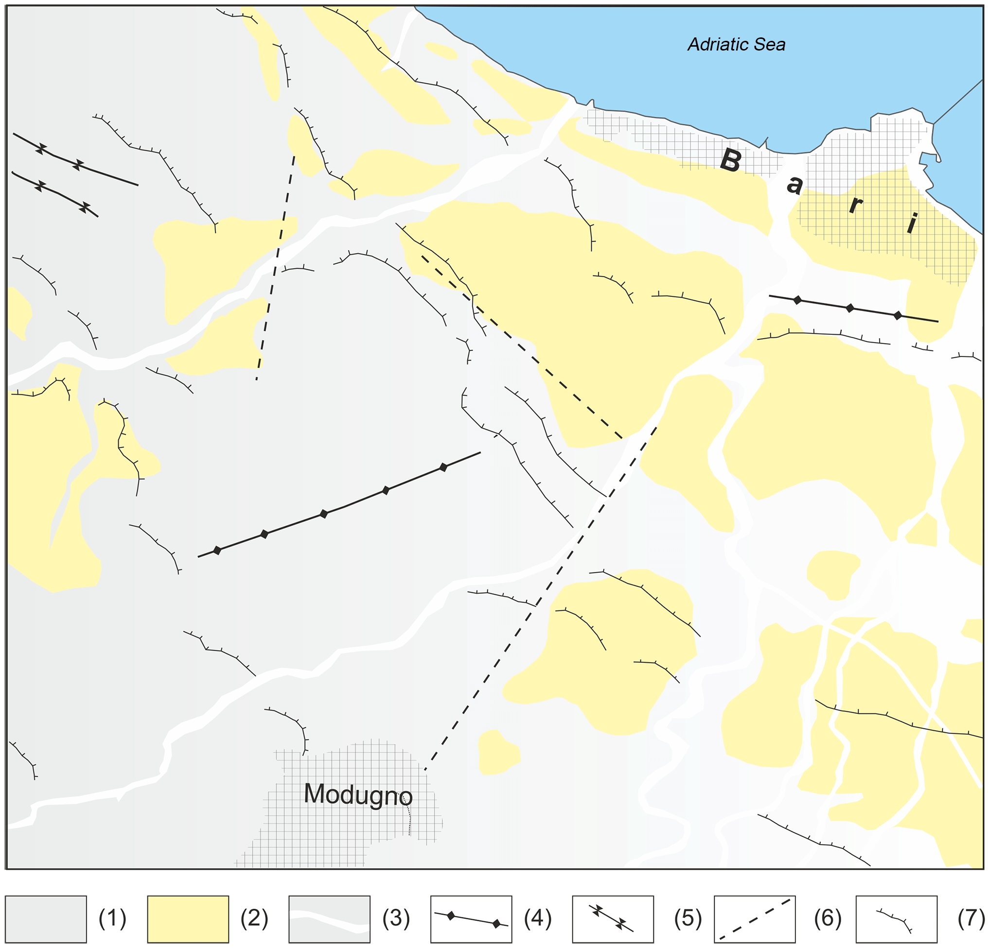
Figure 1Simplified geological map of the area of Bari: (1) Calcare di Bari formation (Cretaceous); (2) Calcareniti di Gravina formation (Lower Pleistocene); (3) hydrographic network; (4) anticlinal axis; (5) syncline axis; (6) fault (uncertain); (7): escarpment.
The effective infiltration has been estimated by means of the hydrologic and hydrogeologic water budget of the subtended basin. Climatic data registered in the thermopluviometric stations present in the area have been elaborated and the average rainfall module and the monthly evapotranspiration have been calculated for the 3 decades 1974–2005.
Twelve climatic stations have been considered (Bari – hydrographic station, Bari – observatory station, Bitonto, Grumo Appula, Adelfia, Casamassima, Mercadante, Ruvo di Puglia, Corato, Altamura, Santeramo, Gioia del Colle) and for each station the monthly rainfall and evapotranspiration map has been realized by means of the inverse distance weighting algorithm. The latter has been estimated by means of the Thornthwaite method, applying a crop coefficient of 0.40.
The hydrologic and hydrogeologic basins have been defined on the basis of literature data and the regional thematic cartography.
The lithotypes in the study area are principally limestones and calcarenites with secondary permeability, characterized by a high transmissivity. The zones in proximity to tectonic structures create preferential flow paths, but at the same time generate a dismemberment of the aquifer that could not be able to feed the flow downstream. Because of that it proves to be difficult to carry out a zonation of recharge areas, and therefore a constant runoff coefficient of 0.10 has been considered for the whole basin. In Fig. 2 the map of the (a) annual precipitation and (b) estimated evapotranspiration evaluated for the hydrological basin of the study area is shown.
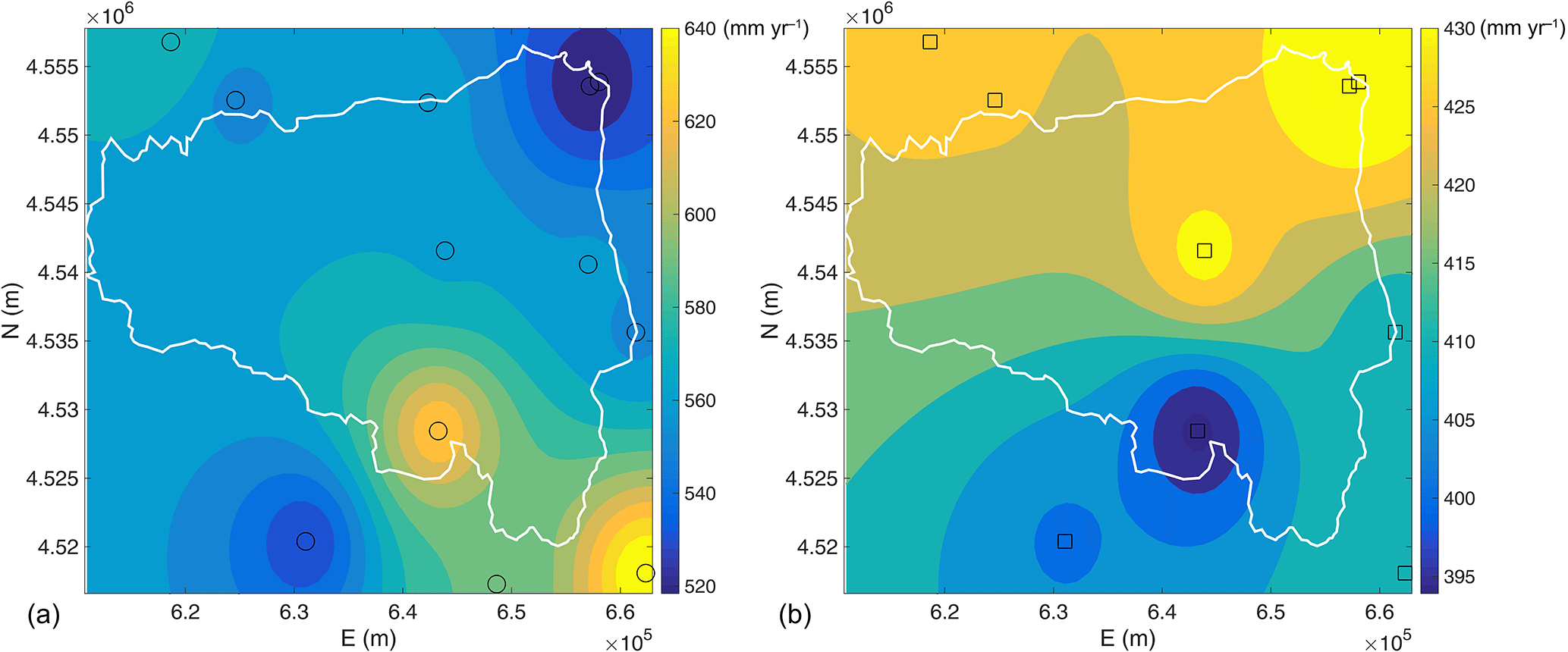
Figure 2Map of (a) annual precipitation and (b) estimated evapotranspiration evaluated for the hydrological basin of the study area.
Ninety-eight long-term step-drawdown hydraulic tests have been analyzed in the study area.
A step-drawdown test is a single-well test in which the well is pumped at a low constant discharge rate until the drawdown within the well stabilizes.
Step-drawdown tests can be used to evaluate the characteristics of the well and its immediate environment. Unlike the aquifer test, it is not designed to produce reliable information concerning the aquifer, even though it is possible to estimate the transmissivity of the immediate surroundings of the catchment. This test determines the critical flow rate of the well, as well as the various head losses and drawdowns as functions of pumping rates and times. Finally, it is designed to estimate the well efficiency, to set an exploitation pumping rate, and to specify the depth of installation of the pump.
The total drawdown at a pumping well is given by
where s (L) represents the registered drawdown, Q (L3 T−1) the pumped flow rate, A1 (T L−2) the linear aquifer loss coefficient, and A2 (T L−2), e, and B (T2 L−5) are, respectively, the linear and nonlinear well-loss coefficients.
This equation can be made explicit in terms of aquifer transmissivity T (L2 T−1), the transmissivity of the damage zone TSKIN (L2 T−1), and the nonlinear term β (T2 L−4) (Cherubini and Pastore, 2011):
where rw (L) represents the well radius, rSKIN (L) the radius of the damage zone, and R (L) the radius of influence of the well.
The total drawdown is formed from three components: the hydraulic component of the aquifer assuming a valid Thiem function, a skin function presented by Cooley and Cunningham (1979) assuming that the transmissivity and the radius of the damage zone are, respectively, equal to e rSKIN=2rw, and a contribution related to nonlinear losses introduced by Wu (2001).
The radius of influence of the well is obtained by means of the Sichart equation:
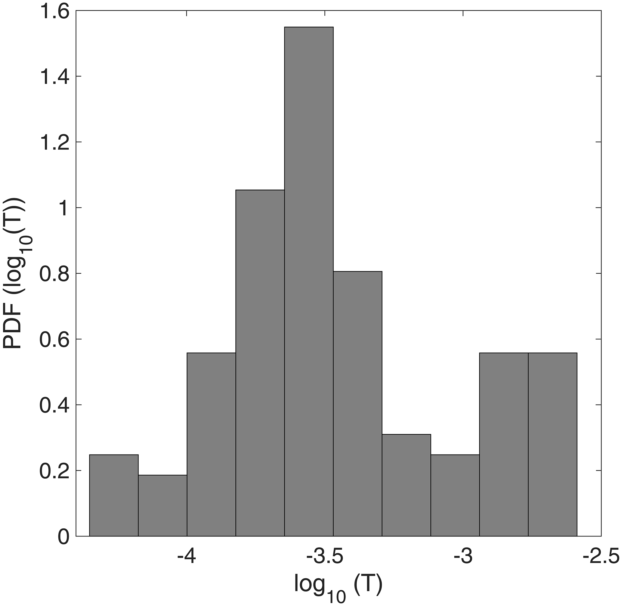
In Fig. 3 is reported the statistical distribution of the estimated transmissivity values along the study area.
The geostatistical analysis has been carried out on the log10 transmissivity values using the S-GemS open-source code (Remy, 2004).
The experimental variogram, which provides a description of how the data are related (correlated) with distance, has been calculated (Fig. 4). Because the Kriging algorithm requires a positive definite model of spatial variability, the experimental variogram cannot be used directly. Instead, a model must be fitted to the data to approximately describe the spatial continuity of the data. An exponential model has been used to fit the experimental variogram described by the function:
where C represents the variance (sill), h (L) the lag, and a (L) the correlation length (range). In our case C assumes a value of 1.2 and a a value of 10000 m.

Figure 4Omnidirectional experimental variogram fitted with an exponential model; sill = 1.2, range = 10000 m.
Figure 5 shows the ordinary Kriging interpolation of log10(T).
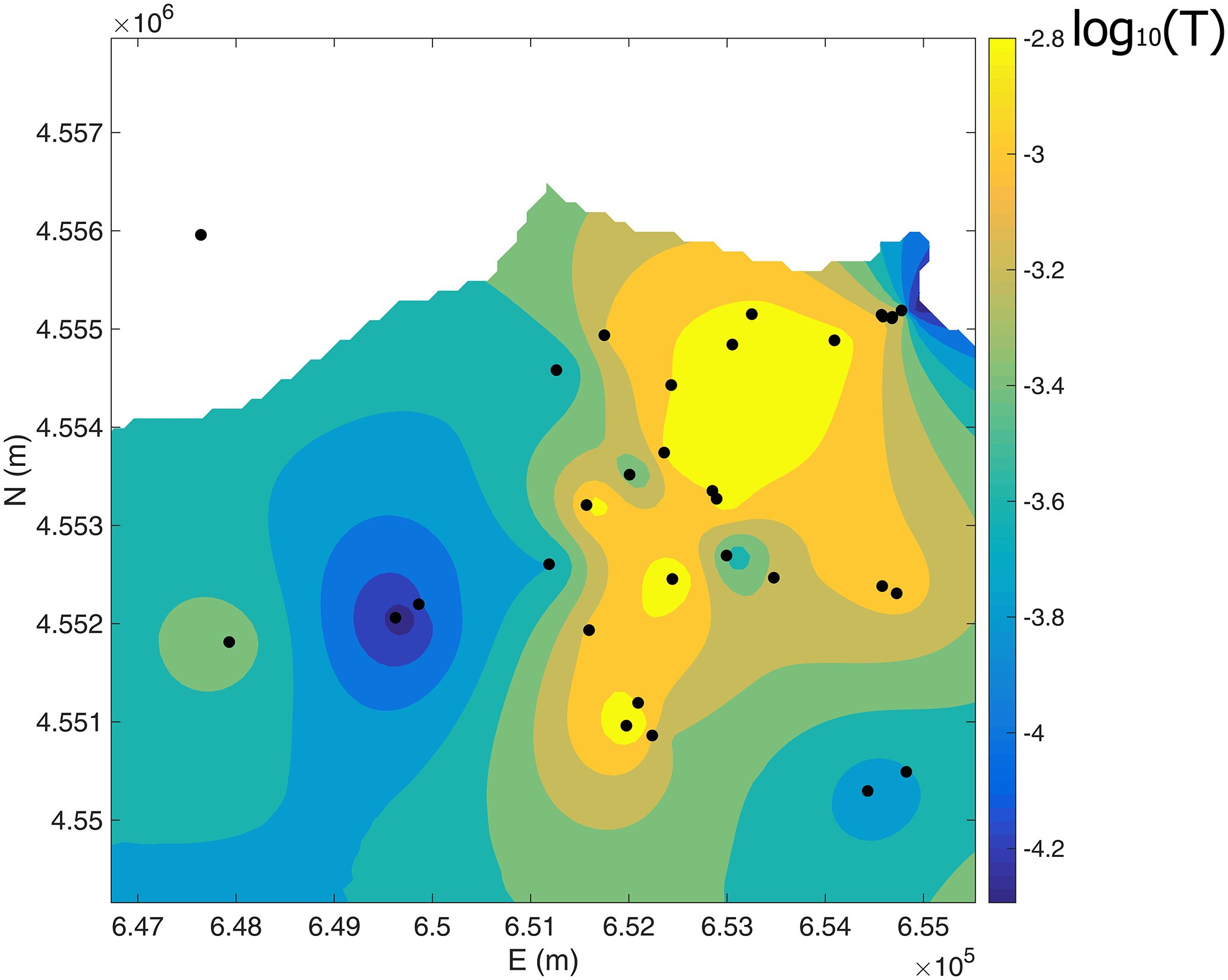
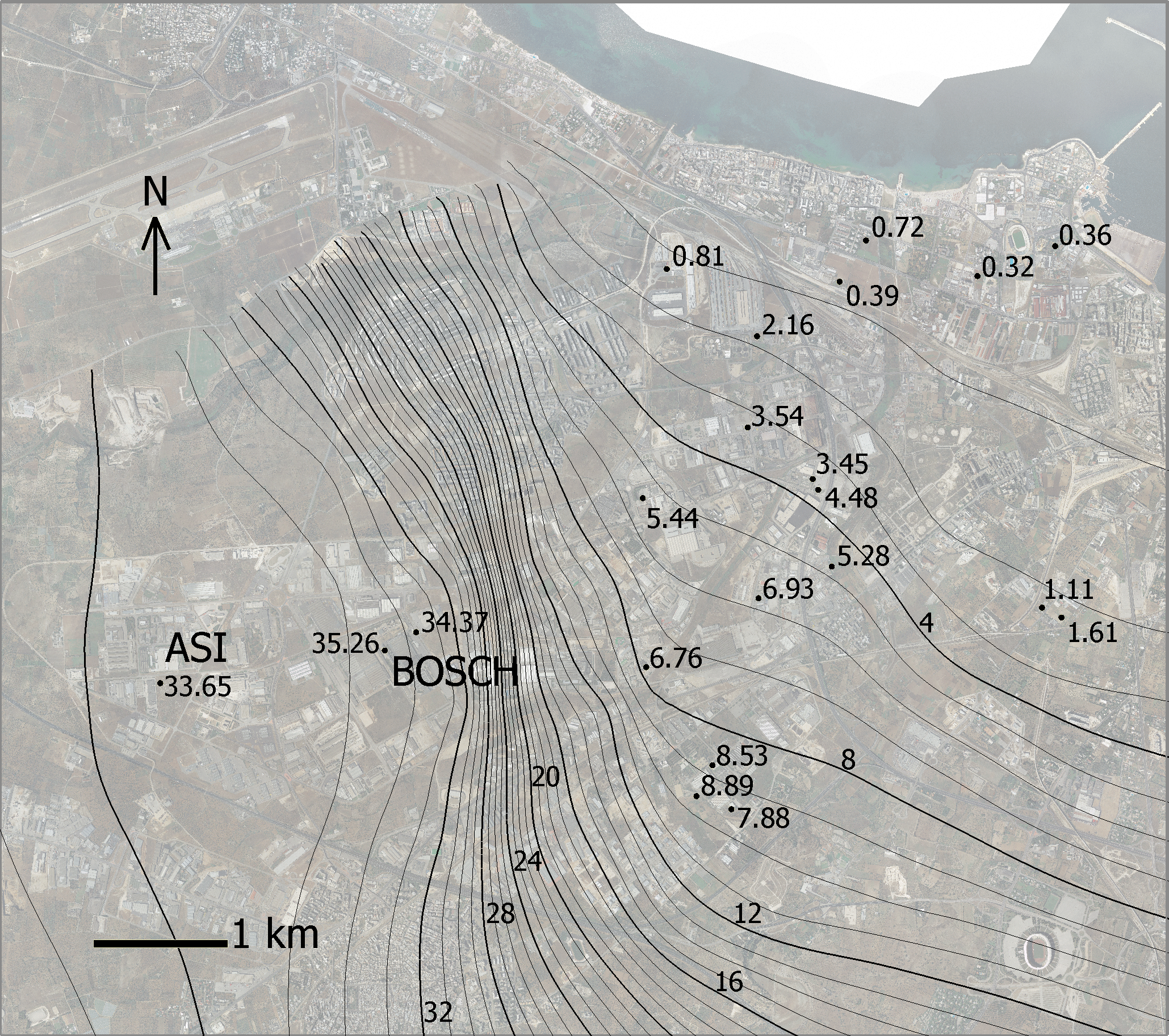
Figure 6 shows the spatial distribution of hydraulic heads on the basis of the 2012 measurement campaign. A global trend in the direction of groundwater flow from SW to NE is evident. A relevant aspect is the presence of high hydraulic head values in proximity to ASI and Bosch wells.
Possible explanations for the increase in hydraulic gradient are (1) lower transmissivity as shown through the step drawdown tests; (2) the transition from a more permeable outcropping lithotype to a less permeable one resulting in a decrease in the effective infiltration; (3) the presence of sinkholes and fissures at the surface giving rise to a point source recharge; and (4) hydraulic disconnection due to lower interconnectivity of the fracture system.
The aquifer transmissivity in that zone is on the order of 10−5 m2 s−1. The trend observed in the hydraulic gradient confirms the increase in the aquifer transmissivity from upstream to downstream: in fact, the tests carried out in proximity to the coast have returned a transmissivity value of 10− to 10−3 m2 s−1.
The various monitoring campaigns carried out have shown a contamination by chlorinated aliphatic hydrocarbons which, unlike petroleum products, are denser than water and can exist as dense non-aqueous phase liquids (DNAPLs).
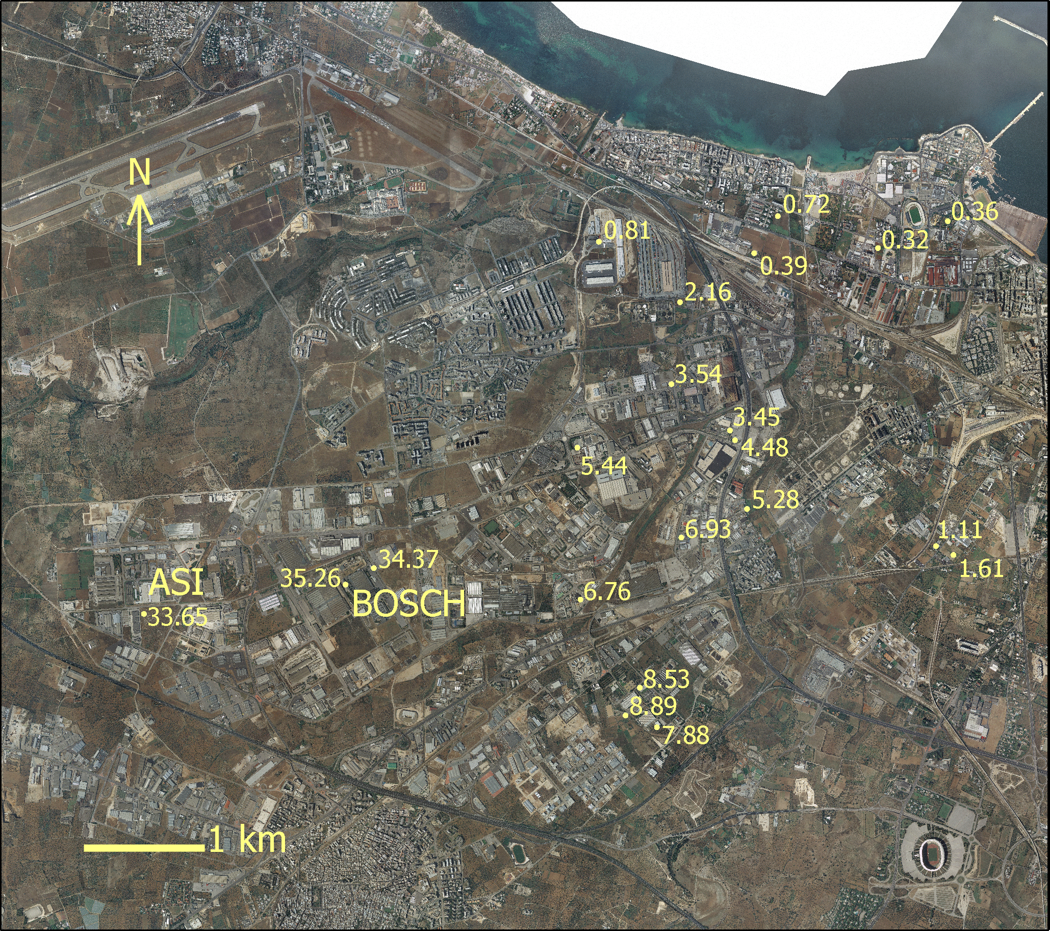
The presence of two hotspot areas has been detected, located upstream of the groundwater flow, coherently with the state of contamination detected downstream.
Figure 7 shows the location of the detected contamination (µg L−1).
The pollution indicator has been chosen on the basis of the toxicologic and cancirogenic parameters, the solubility, the sorption coefficient, and the maximum detected contaminant concentration. On the basis of the results of this screening, the tetrachloroethylene (PCE) has the highest concentration, as well as low values of reference dose factors (RDFs) and slope factors (SFs).
The simplest model of flow through rock fractures is the parallel plate model (Huitt, 1956; Snow, 1965) which conceptualizes the fractured medium as made by a set of smooth parallel plates with the same hydraulic aperture b (L) that are separated by a uniform distance. This is actually the only geometrical fracture model for which an exact calculation of the hydraulic conductivity is possible.
Natural fractures present rough walls and complex geometries. Nonlinear flow may occur through rough walled rock fractures; as a consequence, the inertial effect dominates the flow dynamics, giving rise to a deviation from Darcy's law. Fluid flow through a set of natural fracture planes can be expressed using the Darcy–Weisbach equation:
where D (L) represents the hydraulic diameter (2b for the parallel plate model), f is the Darcy–Weisbach coefficient, h (L) is the hydraulic head, x (L) is the distance, and v (L T−1) is the average velocity in fracture calculated as
where q(L2 T−1) is the volumetric flow rate per unit length of fracture and nf (–) is the number of fractures.
The Darcy–Weisbach equation can be rewritten in terms of volumetric flow per unit length:
The term in square brackets represents the equivalent hydraulic transmissivity Teq(f,∇h) of the nf rough walled fractures.

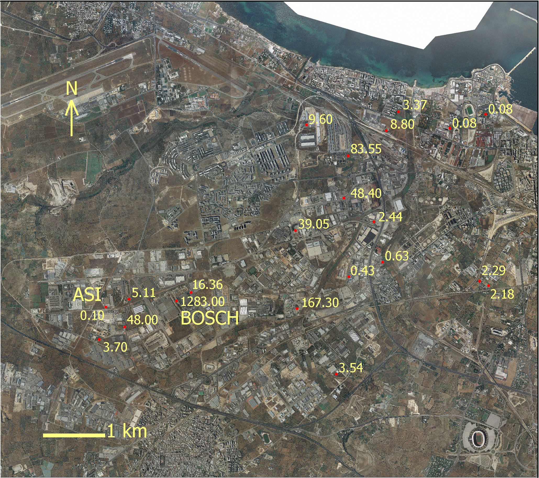
Figure 8Map of log10 of aquifer transmissivity determined by means of the inverse modeling algorithm.

The Darcy–Weisbach coefficient or friction factor depends on the flow regime. In the case of a smooth walled fracture and linear flow regime, f is equal to
where Re represents the Reynolds number:
Substituting Eq. (8) into Eq. (7), the cubic law (Witherspoon et al., 1980) where q is proportional to the cubic power of the fracture aperture is obtained:
The cubic law is not always adequate to represent the flow process in natural fractures, so a deviation from linearity can be observed.
The friction factor depends on the flow regime described by the Reynolds number and can be represented by the following relationship found by Nazridoust at al. (2006):
Inverse modeling is a technique used to estimate unknown model parameters using as input data punctual values of the state variables (hydraulic head flow). Generally, in real problems the number of parameters to estimate (n) is higher than the number of measured values (m). For example, this is the case with mapping hydraulic transmissivity values varying continuously in space.
For underdetermined inverse problems of this kind the objective function (L) can be written in this way:
where s represents the vector of measured values of state variables (e.g. hydraulic transmissivity), and y represents the vector of parameter values.
The fitness function responds to maximum likelihood criteria between the observed and simulated values and can be written as
where h represents the model that, starting from the parameter vector, estimates the state variable, and R is the measurement error covariance matrix. Generally this function can be reduced to the square root of the sum of the squared difference between the measured and simulated RMSE:
where ΔH represents a parameter of accuracy of observed data.
The penalty function is used to discriminate the solutions with values of the fitness function comparable by means of geostatistical criteria (Kitanidis, 1995):
where Q represents the spatial covariance matrix, X is a unit vector, and β is the mean of the values of the parameters. The penalty function can be rewritten by eliminating β:
The common assumption is that the spatial distribution of the parameters follows the geostatistical distribution defined by the variogram. Under this hypothesis the covariance matrix present in the penalty function can be defined as
Solute transport in fracture neglecting the effect of matrix diffusion and the chemical reactions can be described by the following advection–dispersion equation:
where c (M L−3) is the concentration of a solute and D (L2 T−1) is the symmetric dispersion tensor with the following components:
where αL (L) and αT (L) are the longitudinal and transverse dispersivities, respectively.
For pure advective transport the particle moves along the flow lines. In order to represent dispersion phenomena, the random walk method adds a random displacement to each particle, independently of the other particles, in addition to advective displacement.
For a given time step Δt, considering the tensorial nature of the dispersion and the spatially variable velocity field, each particle moves according to
with
where Z1 and Z2 are two normally distributed random variables. For steady-state flow and for a source constant intensity, the assumption that the particles N released in time interval (t1, t1+Δt) follow exactly the same random trajectories of the particles N released during the previous interval (t1, t1−Δt) is possible. Under this assumption only N particles are needed to simulate the location of the particles at a previous time step.
11.1 Flow modeling
The MODFLOW numerical code coupled with the inverse model approach presented in the previous section has been used to model groundwater flow.
The numerical simulations have been carried out on a two-dimensional domain of 968.7 km2. The domain has been discretized by means of a structured grid of 100 m in size.
In correspondence to the coastline, a first type of boundary condition has been imposed (h=0 m), and along the detected watershed a second type of boundary condition (q=0 m2 s−1); the recharge from upstream is simulated by means of a first type of boundary condition where the hydraulic heads are equal to the detected regional values h=32–41 m (Piano di Tutela delle Acque Regione Puglia, Tav. 6.2 http://old.regione.puglia.it/index.php?page=documenti&id=29&opz=getdoc, last access: February 2018).
A second type of boundary condition on the whole simulation domain has been imposed that concerns the mean effective infiltration calculated from the hydrologic budget q=0.037 m3 d−1.
The algorithm of inverse modeling has been applied to carry out the estimation of the spatial distribution of the equivalent transmissivity (Fig. 8) on the basis of the observed hydraulic head (vector y), the regionalization model (matrix Q) described by the variogram of the logarithm of the hydraulic transmissivity determined in the previous section.
The inverse model algorithm follows those steps. (1) Start from a conditional simulation of the log of Teq determined by means of the hydraulic tests conducted in the area. (2) A set of pilot points are chosen in the area using a regularly spaced criterion and the value of Teq has been determined for each pilot point (vector s). (3) By means of the ordinary Kriging interpolation of the pilot points the map of Teq is obtained and represents the input datum of the flow numerical model. (4) The hydraulic head has been determined using the flow numerical model (vector h) and the values of the objective function have been determined using Eq. (12). (5) The values of Teq are updated for each pilot point.
Using the Levenberg–Marquardt algorithm, the values of Teq for each pilot point are updated as long as the objective function is minimized.
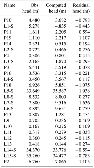
Figure 9 shows the results obtained from the flow model in steady-state condition, calibrated with the measurement campaign of February 2012 (Table 1).
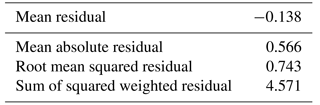
Table 2 shows the data of model calibration and Fig. 10 shows the graph of the calibration.
The outcomes of the calibration are satisfactory. The comparison between the simulated and observed data has given a mean absolute residual equal to 0.57 m, an RMSE equal to 4.57 m, and a correlation coefficient r2 equal to 0.997. In the following figures and tables are shown the results for the flow model.
Table 1Comparison between the observed and simulated hydraulic heads with related residuals, relative to the measurement campaign of February 2012.
The simulated hydraulic head distribution together with the equivalent transmissivity map put into evidence how the anticline affecting the Calcare di Bari formation in direction ENE–WSW influences the flow directions. Furthermore, they highlight how the hydraulic circulation is more active along the coast coherently with a higher degree of fracturing and karst phenomena.
Once the equivalent hydraulic transmissivity map has been obtained, and assuming a value of the number of sets of fractures nf, the spatial distribution of the mean equivalent aperture and the velocity field can be obtained.
Assuming the cubic law to be valid, the mean equivalent aperture can be obtained as
The velocity field results:
whereas assuming the Darcy–Weisbach equation to be valid, the mean equivalent aperture and the flow field can be obtained by means of the following iterative steps starting from the values of beq, vx, and vy previously evaluated:
Figure 11 shows the relative percentage of error in the flow velocity magnitude for different numbers of fractures.
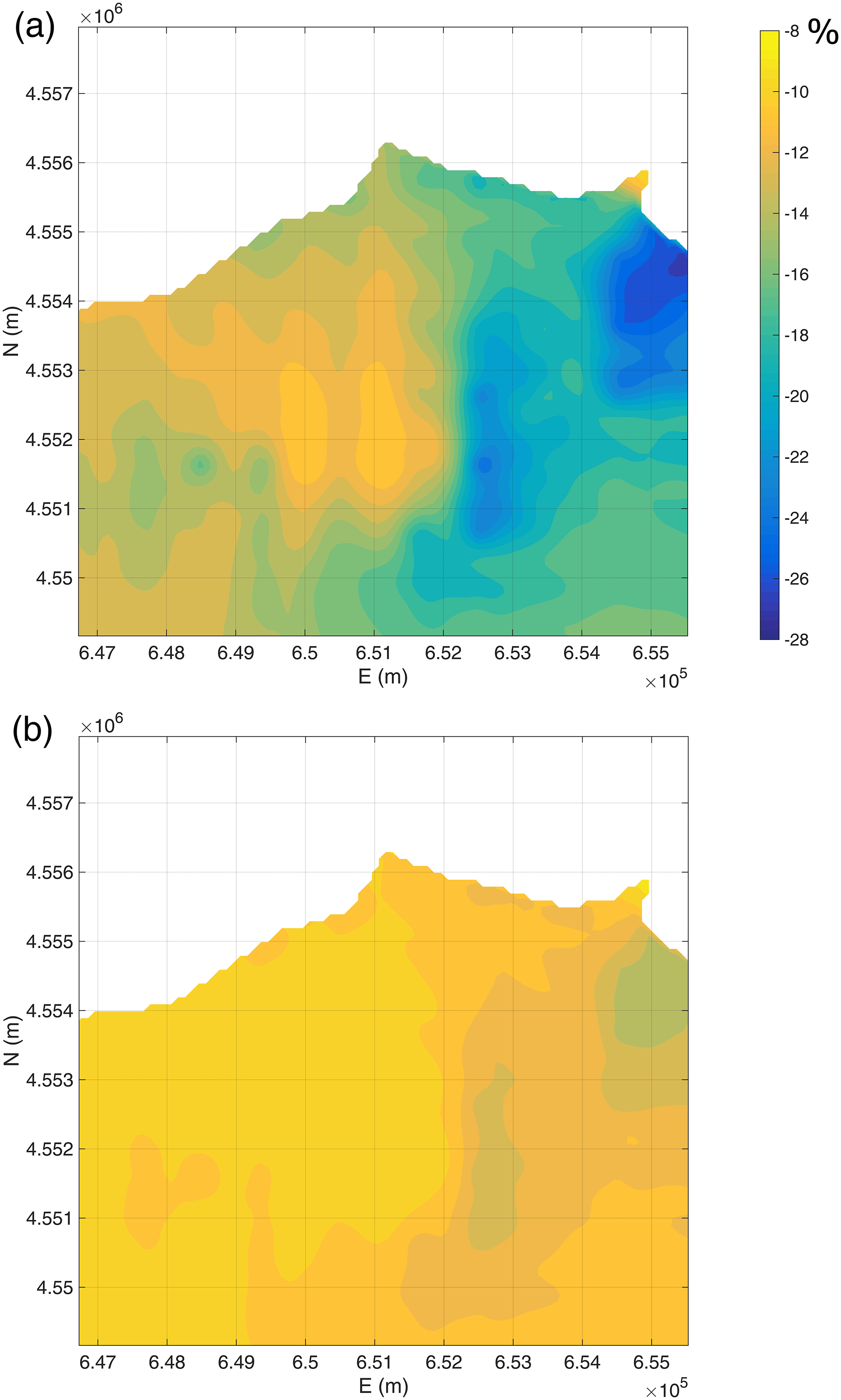
Figure 11Relative percentage of error in the flow velocity magnitude for different numbers of fractures: (a) nf= 4; (b) nf= 28.

Figure 12Steady-state distribution of hypothetical contamination using the random walk model with the source contamination localized in correspondence to the hotspot of the contamination considering a number of fracture of nf= 20 and a longitudinal and transversal dispersion coefficient equal to αL= 70 m and αT= 7 m.

Figure 13Breakthrough curves of hypothetical continuous contamination released in correspondence to the hotspot, determined for linear and nonlinear flow models, evaluated at the downstream boundary.
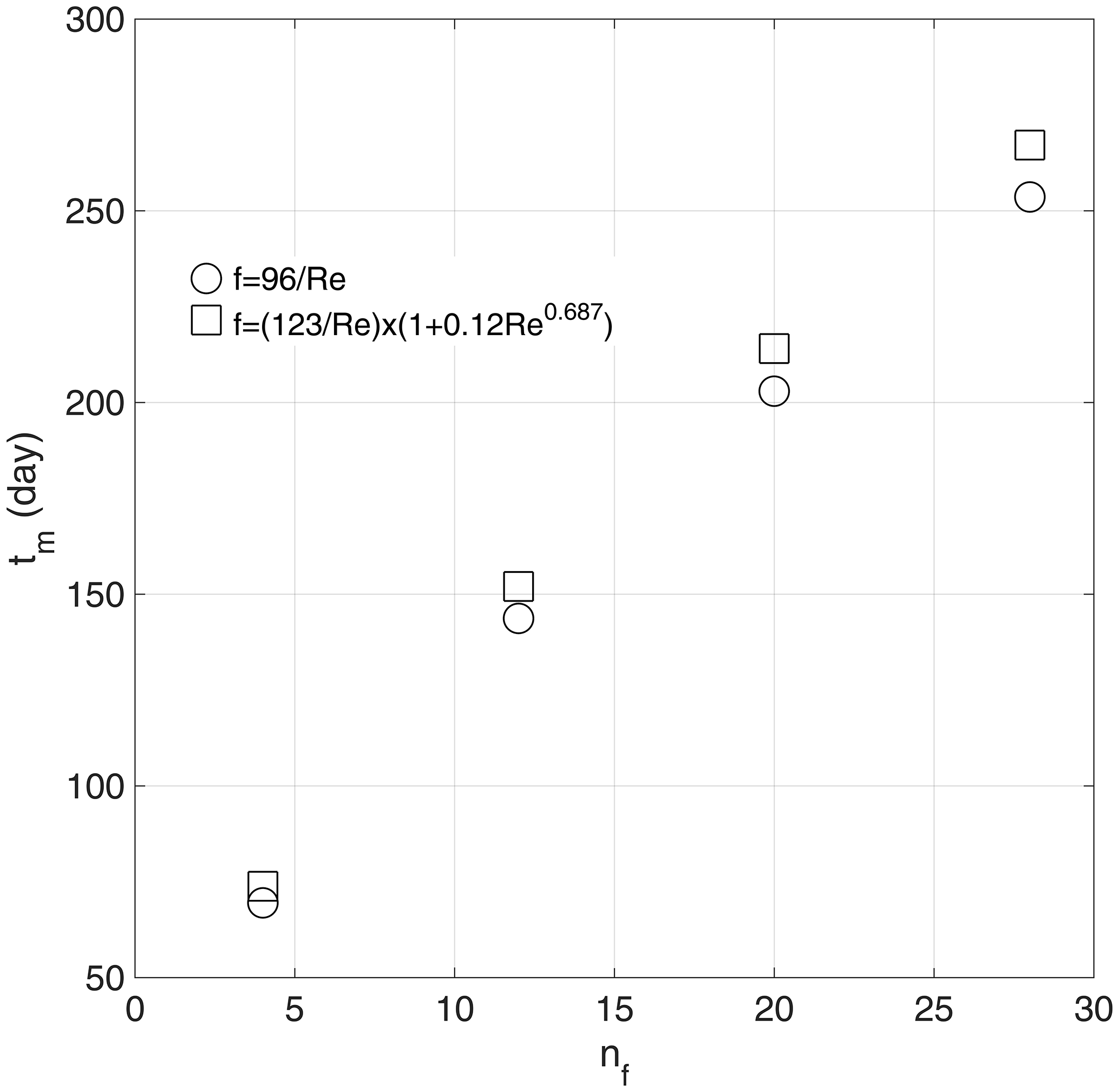
Figure 14Mean travel time tm at varying numbers of fractures nf for linear and nonlinear models.
As the number of fractures increases, the velocity magnitude decreases; therefore, the friction factor reaches a value of 96∕Re. Anyway, the percentage of error in the flow velocity magnitude seems not to be negligible. In fact, for nf=28 a minimum value of 8 % is obtained, reaching a value of 28 % for nf=4. These results show that under natural hydraulic gradient conditions in fractured limestone the nonlinearity of the flow cannot be negligible. It is clear that under a forced hydraulic gradient due to anthropic stresses the equivalent transmissivity decreases dramatically, with a value less than 40 % of Darcian-like hydraulic transmissivity (Cherubini et al., 2012).
11.2 Analysis of the scenario of contamination
A particle tracking transport method has been applied for the simulation of contaminant transport. A punctual source contamination has been imposed in correspondence to the detected hotspot equal to a PCE concentration of 1283 µg L−1. This localization is coherent with the soil contamination detected in the area.
In order to solve the advective transport equation a numerical Lagrangian particle-based random walk method is implemented. For each time step a constant number of 500 particles have been released into the domain from the source. According to the Rauch et al. (2005) assumption reported in the previous section, only 500 particles are needed to simulate the steady-state distribution of the hypothetical contamination. Even if the source of contamination has been considered punctual, the obtained simulation scenario proves to be compatible with the observed one, and therefore it is possible to assume that the sources of contamination are located in correspondence to the detected hotspot (Fig. 12).
Figure 13 shows the breakthrough curves of hypothetical continuous contamination released in correspondence to the hotspot, determined for linear and nonlinear flow models, evaluated at the downstream boundary for nf = 20.
Figure 14 shows the mean travel time at a varying number of fractures for the linear and nonlinear models. With an increasing number of fractures, the travel time increases in a linear way, because the cross-sectional area increases as well. The figures highlight that travel time for the nonlinear model is higher than the linear assumption. In a particular way, the percentages of error are in the range of 6.22 %–5.34 % passing from nf= 4 (Re = 0.02–10.60) to nf=28 (Re = 0.002–1.51). This is coherent with what was detected by Cherubini et al. (2012, 2013b, 2014), who carried out hydraulic and tracer tests on an artificially created fractured rock sample and found a pronounced mobile–immobile zone interaction leading to a non-equilibrium behavior of solute transport.
The existence of a non-Darcian flow regime was shown to influence the velocity field by giving rise to a delay in solute migration with respect to the values that could be obtained under the assumption of a linear flow field. Furthermore, the presence of inertial effects was shown to enhance non-equilibrium behavior. In a particular manner, they found that the percentage of error in the travel time with respect to the linear flow assumption varied in the range of 5.90 %–40.75 %, corresponding to a range of Re of 29.48–52.16. These results highlight the fact that as the scale of observation increases, the error in the mean travel time with respect to the linear flow model becomes more relevant. In fact, at field scale also for Re, just above the unit (nf = 28), the error is equal to 5.34 %, comparable with the error of 5.90 % found at laboratory scale for Re equal to 29.48. This means that under anthropic stresses multiple pumpings or injections give rise to a higher flow velocity and then higher Re, leading to a dramatic delay on contaminant transport. Therefore, nonlinear flow must be considered in order to have a more accurate estimation of the breakthrough curve and mean travel time of contaminated scenarios.
In fracture networks, the presence of nonlinear flow plays an important role in the distribution of the solutes according to the different pathways. In fact, the energy spent to cross the path should be proportional to the resistance to flow associated with the single pathway, which in a nonlinear flow regime is not constant but depends on the flow rate. This means that by changing the boundary conditions, the resistance to flow varies and consequently the distribution of solute in the main and secondary pathways also changes, giving rise to a different behavior of solute transport (Cherubini et al., 2014).
This concept has to be taken into account in case of cleanup of the aquifer using for example the Pump & Treat system. The multiple pumping and reinjection of the treated groundwater give rise to a higher flow velocity in the aquifer, resulting in a much greater hydraulic gradient. In this case nonlinear flow behavior has to be taken into account in order to obtain more accurate cleanup strategies.
The present study is aimed at analyzing the scenario of groundwater contamination (by investigating the hotspots) of the industrial area of Modugno (Bari – southern Italy) where the limestone aquifer has a fractured and karstic nature.
The presence of hotspot areas has been detected, located upstream of the groundwater flow, coherently with the state of contamination detected downstream and the soil contamination.
A rough walled parallel plate model has been implemented and calibrated on the basis of piezometric data and has coupled a geostatistical analysis to infer the values of the equivalent aperture. Using the random walk theory, the steady-state distribution of hypothetical contamination with the source contamination at the hotspot has been carried out.
The flow and transport models have reproduced the flow pattern well and have given a pollution scenario that is compatible with the observed one.
From an analysis of the flow and transport pattern it is possible to infer that the anticline affecting the Calcare di Bari formation in direction ENE–WSW influences the direction of flow as well as the propagation of the contaminant.
The results also show that the presence of nonlinear flow influences advection, in that it leads to a delay in solute transport with respect to the linear flow assumption. Moreover, the distribution of solute according to different pathways is not constant, but is related to the flow rate.
This is due to the non-proportionality between the energy spent to cross the path and the resistance to flow for fractured media, which affects the distribution of the solutes according to the different pathways.
The obtained results represent the fundamental basis for a detailed study of the contaminant propagation in correspondence to the hotspot area in order to find the best cleanup strategies and optimize any anthropic intervention on the industrial site.
Future developments of the current study will be to implement a transient model and to include the density-dependent flow in the simulations.
Research data can be publicly accessed in the Supplement to this paper.
The supplement related to this article is available online at: https://doi.org/10.5194/hess-22-5211-2018-supplement.
CC and NP dealt with data analysis, modeling and interpretation, DR dealt with the geology part and interpretation of results, and CIG dealt with interpretation of results and theoretical analysis.
The authors declare that they have no conflict of interest.
The authors would like to acknowledge the editor and reviewers for their
valuable comments and suggestions that helped improve the
manuscript.
Edited by: Philippe Ackerer
Reviewed by: Eric Zechner and
Nicole Sund
Antonellini, M., Cilona, A., Tondi, E., Zambrano, M., and Agosta, F.: Fluid-flow numerical experiments of faulted porous carbonates, Northwest Sicily (Italy), Mar. Petrol. Geol., 55, 186–201, 2014.
Baker, W. J.: Flow in fissured formations, Proceedings of 4th Worm Petroleum Congress, Carlo Colombo, Rome, 379–393, 1955.
Berkowitz, B., Kosakowski, G., Margolin, G., and Scher, H.: Application of Continuous Time Random Walk Theory to Tracer Test Measurements in Fractured and Heterogeneous Porous Media, Ground Water, 39, 593–603, 2001.
Bieniawski, Z. T.: Engineering Rock Mass Classifications, John Wiley & Sons, New York, 251, 1989.
Billi, A., Salvini, F., and Storti, F.: The damage zone-fault core transition in carbonate rocks: implications for fault growth, structure and permeability, J. Struct. Geol., 25, 1779–1794, 2003.
Brush, D. J. and Thomson, N. R.: Fluid flow in synthetic rough-walled fractures: Navier-Stokes, Stokes, and local cubic law simulations, Water Resour. Res., 39, 1085, https://doi.org/10.1029/2002WR001346, 2003.
Bourke, P. J.: Channeling of flow through fractures in rock, in Proceedings of GEOVAL-1987 International Symposium, 1, Swedish Nuclear Power Inspectorate (SKI), Stockholm, 167–177, 1987.
Caine, J. S. and Forster, C. B.: Fault zone architecture and fluid flow: Insights from field data and numerical modeling, in: Faults and sub-surface fluid flow in the shallow crust, edited by: Haneberg, W. C., Mozley, P. S., Moore, C., and Goodwin, L. B., AGU Geophysical Monograph, 113, 101–127, 1999.
Caine, J. S., Evans, J. P., and Forster, C.: Fault zone architecture and permeability structure, Geology, 24, 1025–1028, 1996.
Cherubini, C.: A modeling approach for the study of contamination in a fractured aquifer, Geotechnical and geological engineering, Springer, the Netherlands, 26, 519–533, 2008.
Cherubini, C. and Pastore, N.: Modeling contaminant propagation in a fractured and karstic aquifer, Fresen. Environ. Bull., 19, 1788–1794, 2010.
Cherubini, C. and Pastore, N.: Critical stress scenarios for a coastal aquifer in southeastern Italy, Nat. Hazards Earth Syst. Sci., 11, 1381–1393, https://doi.org/10.5194/nhess-11-1381-2011, 2011.
Cherubini, C., Pastore, N., and Francani, V.: Different approaches for the characterization of a fractured karst aquifer, World scientific and engineering academy and society, Transactions on fluid mechanics, Wisconsin-Usa, 1, 29–35, 2008.
Cherubini, C., Giasi, C. I., and Pastore, N.: Bench scale laboratory tests to analyze non-linear flow in fractured media, Hydrol. Earth Syst. Sci., 16, 2511–2522, https://doi.org/10.5194/hess-16-2511-2012, 2012.
Cherubini, C., Giasi, C., and Pastore, N.: Fluid flow modeling of a coastal fractured karstic aquifer by means of a lumped parameter approach, Environ. Earth Sci., 70, 2055–2060, 2013a.
Cherubini, C., Giasi, C. I., and Pastore, N.: Evidence of non-Darcy flow and non-Fickian transport in fractured media at laboratory scale, Hydrol. Earth Syst. Sci., 17, 2599–2611, https://doi.org/10.5194/hess-17-2599-2013, 2013b.
Cherubini, C., Giasi, C. I., and Pastore, N.: On the reliability of analytical models to predict solute transport in a fracture network, Hydrol. Earth Syst. Sci., 18, 2359–2374, https://doi.org/10.5194/hess-18-2359-2014, 2014.
Cooley, R. L. and Cunningham, A. B.: Consideration of energy loss in theory of flow to wells, J. Hydrol., 43, 161–184, 1979.
Cortis, A. and Birkholzer, J.: Continuous time random walk analysis of solute transport in fractured porous media, Water Resour. Res., 44, W06414, https://doi.org/10.1029/2007WR006596, 2008.
Deere, D. U. and Deere, D. W.: The rock quality designation (RQD) index in practice, Rock classification systems for engineering purposes, edited by: Kirkaldie, L., ASTM Special Publication Philadelphia, Am. Soc. Test. Mater., 984, 91–101, 1988.
Dentz, M., Kang, P. K., and Le Borgne, T.: Continuous Time Random Walks for Non-Local Radial Solute Transport, Adv. Water Resour., 82, 16–26, 2015.
Diersch, H. J. G.: FEFLOW finite element subsurface flow and transport simulation system, User's manual/Reference manual/White papers, Release 5.1, WASY Ltd, Berlin, 2002.
Doglioni, C.: The Puglia uplift (SE Italy) An anomaly in the foreland of the Apenninic subduction due to buckling of a thick continental lithosphere, Tectonics, 13, 1309–1321, 1994.
Elliott, G. M. and Brown, E. T.: Laboratory measurement of the thermo-hydro-mechanical properties of rock, Q. J. Eng. Geol. Hydroge., 21, 299–314, 1988.
Forster, C. B. and Evans, J. P.: Hydrogeology of thrust faults and crystalline thrust sheets: results of combines field and modelling studies, Geophys. Res. Lett., 18, 979–982, 1991.
Gale, J. A.: Numerical Field and Laboratory Study of Flow in Rocks with Deformable Fractures, Sci. Ser. 72, Inland Waters Dir., Water Resources Branch, Ottawa, Ontario, Canada, 1977.
Huitt, J. L.: Fluid Flow in Simulated Fractures, Amer. Inst. Chem. Eng. J., 2, 259–264, 1956.
Lee, J., Kang, J. M., and Choe, J.: Experimental analysis on the effects of variable apertures on tracer transport, Water Resour. Res., 39, 1015, https://doi.org/10.1029/2001WR001246, 2003.
Keller, A.: High resolution, non-destructive measurement and characterization of fracture apertures, Int. J. Rock Mech. Min., 35, 1037–1050, 1998.
Keller, A. A., Roberts, P. V., and Blunt, M. J.: Effect of fracture aperture variations on the dispersion of contaminants, Water Resour. Res., 35, 55–63, 1999.
Kitanidis, P.: Quasi?linear geostatistical theory for inversing, Water Resour. Res., 31, 2411–2419, https://doi.org/10.1029/95WR01945, 1995.
Klimczak, C., Schultz, R. A., Parashar, R., and Reeves, D. M.: Cubic law with aperture-length correlation: implications for network scale fluid flow, Hydrogeol. J., 18, 851–862, 2010.
Korneva, I., Tondi, E., Agosta, F., Rusctichelli, A., Spina, V., Bitonte, R., and Di Cuia, R.: Structural properties of fractured and faulted Cretaceous platform carbonates, Murge Plateau (Southern Italy), Mar. Petrol. Geol., 57, 312–326, 2014.
Masciopinto, C. and Palmiotta, D.: Flow and Transport in Fractured Aquifers: New Conceptual Models Based on Field Measurements, Transport Porous Med., 96, 117–133, 2013.
Masciopinto, C. and Visino, F.: Strong release of viruses in fracture flow in response to a perturbation in ionic strength: Filtration/retention tests and modeling, Water Res., 126, 240–251, 2017.
Masciopinto, C., Volpe, A., Palmiotta, D., and Cherubini, C.: A combined PHREEQC-2/parallel fracture model for the simulation of laminar/non-laminar flow and contaminant transport with reactions, J. Contam. Hydrol., 117, 94–108, 2010.
Nazridoust, K., Ahmadi, G., and Smith, D. H.: A new friction factor correlation for laminar, single-phase flows through rock fractures, J. Hydrol., 329, 315–328, https://doi.org/10.1016/j.jhydrol.2006.02.032, 2006.
Neretnieks, I., Eriksen, T., and Tahtinen, P.: Tracer movement in a single fissure in granitic rock: Some experimental results and their interpretation, Water Resour. Res., 18, 849–858, 1982.
Neuzil, C. E. and Tracy, J. V.: Flow Through Fractures, Water Resour. Res., 17, 191–199, 1981.
Oron, A. P. and Berkowitz, B.: Flow in rock fractures: The local cubic law assumption reexamined, Water Resour. Res., 34, 2811–2825, 1998.
Parise, M. and Pascali, V.: Surface and subsurface environmental degradation in the karst of Apulia (southern Italy), Environ. Geol., 44, 247–256, 2003.
Pieri, P., Festa, V., Moretti, M., and Tropeano, M.: Quaternary tectonic activity of the Murge area (Apulian foreland-Southern Italy), Ann. Geofis., 40, 1395–1404, 1997.
Pieri, P., Sabato, L., Spalluto, L., and Tropeano, M.: Note Illustrative della Carta Geologica d'Italia alla scala 1:50.000 foglio 438, Bari, Nuova Carta Geologica d'Italia alla scala 1:50.000 – Progetto CARG, ISPRA-Servizio Geologico d'Italia, ISBN 2035-8008, January 2012.
Plouraboué, F., Kurowski, P. J., Hulin, P., Roux, S., and Schmittbuhl, J.: Aperture of rough crack, Phys. Rev., 51, 1675–1685, 1995.
Plouraboué, F., Kurowski, P., Boffa, J. M., Hulin, J. P., and Roux, S.: Experimental study of the transport properties of rough self-affine fractures, J. Contam. Hydrol., 46, 295–318, 2000.
Priest, S. D. and Hudson, J. A.: Discontinuity spacings in rock, Int. J. Rock Mech. Min., 13, 135–148, 1976.
Pyrak-Nolte, L. J., Cook, N. G. W., and Nolte, D.: Fluid percolation through single fractures, Geophys. Res. Lett., 15, 1247–1250, 1988.
Rauch, R., Schäfer, W., and Wagner, C.: Solute Transport Modelling. An introduction to Models and Solution Strategies, Gebrüder Borntraeger Verlagsbuchhandlung, Berlin Tuggart, 2005.
Remy, N.: Geostatistical Earth Modeling Software: User's Manual, Stanford University, 15–18, available at: http://sgems.sourceforge.net/ (last access: July 2018), 2004.
Rustichelli, A., Tondi, E., Agosta, F., Cilona, A., and Giorgioni, M.: Development and distribution of bed-parallel compaction bands and pressure solution seams in carbonates (Bolognano Formation, Majella Mountain, Italy), J. Struct. Geol., 37, 181–199, 2012.
Snow, D. T.: A Parallel Plate Model of Fractured Permeable Media, PhD Dissertation, University of California, 1965.
Snow, D. T.: The Frequency and Apertures of Fractures in Rocks, Int. J. Rock Mech. Min., 7, 23–40, 1970.
Srinivasan, G., Tartakovsky, D. M., Dentz, M., Viswanathan, H., Berkowitz, B., and Robinson, B. A.: Random walk particle tracking simulations of non-Fickian transport in heterogeneous media, J. Comput. Phys., 229, 4304–4314, 2010.
Tsang, Y. W. and Tsang, C. F.: Channel model of flow through fractured media, Water Resour. Res., 23, 467–479, 1987.
Tsang, Y. W. and Tsang, C.-F.: Flow channeling in a single fracture as two-dimensional strongly heterogeneous permeable medium, Water Resour. Res., 25, 2076–2080, 1989.
Tsang, C.-F., Tsang, Y. W., Birkhölzer, J., and Moreno, L.: Dynamic channeling of flow and transport in saturated and unsaturated heterogeneous media, in Flow and Transport Through Unsaturated Fractured Rock, 2nd ed., Geophys. Monograph, 42, 33–44, AGU, Washington, D.C., 2001.
Wang, L., Cardenas, M. B., Slottke, D. T., Ketcham, R. A., and Sharp Jr., J. M.: Modification of the Local Cubic Law of fracture flow for weak inertia, tortuosity and roughness, Water Resour. Res., 51, 2064–2080, 2015.
Witherspoon, P. A., Wang, J. S. Y., Iwai, K., and Gale, J. E.: Validity of the cubic law for fluid flow in a deformable rock fracture, Water Resour. Res., 16, 1016–1034, 1980.
Wu, Y. S.: NonDarcy Displacement of Immiscible Fluids in Porous Media, Water Resour. Res., 37, 2943–2950, https://doi.org/10.1029/2001WR000389, 2001.
Zhang, X. and Spiers, C. J.: Compaction of granular calcite by pressure solution at room temperature and effects of pore fluid chemistry, Int. J. Rock Mech. Min., 42, 950–960, 2005.
Zheng, Q., Dickson, S. E., and Guo, Y.: On the appropriate “equivalent aperture” for the description of solute transport in single fractures: Laboratory-scale experiments, Water Resour. Res., 44, W04502, https://doi.org/10.1029/2007WR005970, 2008.
Zimmerman, R. W. and Bodvarsson, G. S.: Hydraulic conductivity of rock fractures, Transpot Porous Med., 23, 1–30, 1996.
- Abstract
- Introduction
- Geological and hydrogeological framework
- Hydrologic and hydrogeologic water budget
- Well-performance tests: step-drawdown tests
- Linear model of regionalization of transmissivity
- Analysis of piezometric data
- Analysis of the scenario of contamination for the study area
- Parallel rough walled fracture model
- Inverse flow modeling
- Solute transport modeling
- Results and discussion
- Conclusions
- Data availability
- Author contributions
- Competing interests
- Acknowledgements
- References
- Supplement