Evaluation of impacts of future climate change and water use scenarios on regional hydrology

General circulation models (GCMs) have been widely used to simulate current and future climate at the global scale. However, the development of frameworks to apply GCMs to assess potential climate change impacts on regional hydrologic systems, ability to meet future water demand, and compliance with water resource regulations is more recent. In this study eight GCMs were bias-corrected and downscaled using the bias correction and stochastic analog (BCSA) downscaling method and then used, together with three ET₀ methods and eight different water use scenarios, to drive an integrated hydrologic model previously developed for the Tampa Bay region in western central Florida. Variance-based sensitivity analysis showed that changes in projected streamflow were very sensitive to GCM selection, but relatively insensitive to ET₀ method or water use scenario. Changes in projections of groundwater level were sensitive to both GCM and water use scenario, but relatively insensitive to ET₀ method. Five of eight GCMs projected a decrease in streamflow and groundwater availability in the future regardless of water use scenario or ET method. For the business as usual water use scenario all eight GCMs indicated that, even with active water conservation programs, increases in public water demand projected for 2045 could not be met from ground and surface water supplies while achieving current groundwater level and surface water flow regulations. With adoption of 40 % wastewater reuse for public supply and active conservation four of the eight GCMs indicate that 2045 public water demand could be met while achieving current environmental regulations; however, drier climates would require a switch from groundwater to surface water use. These results indicate a high probability of a reduction in future freshwater supply in the Tampa Bay region if environmental regulations intended to protect current aquatic ecosystems do not adapt to the changing climate. Broad interpretation of the results of this study may be limited by the fact that all future water use scenarios assumed that increases in water demand would be the result of intensification of water use on existing agricultural, industrial, and urban lands. Future work should evaluate the impacts of a range of potential land use change scenarios, with associated water use change projections, over a larger number of GCMs.

1 Introduction

The Intergovernmental Panel on Climate Change (IPCC) along with many other studies have indicated that climate change is likely to alter both the global hydrologic cycle and regional hydrologic cycles (Aalst et al., 2014; Déry et al., 2009; Georgakakos et al., 2014; Hawkins et al., 2014; Milliman et al., 2008). These studies have indicated that climate change is likely to increase the frequency of droughts, as well as the magnitude of floods in many regions (Diffenbaugh and Field, 2013; Georgakakos et al., 2014; Walsh et al., 2014). It is necessary to investigate future climate change and its potential impacts on the natural environment in order to reduce risks and increase resilience for future water resource planning and management (Vano and Lettenmaier, 2013).

General circulation models (GCMs) and hydrologic models have been widely used to evaluate future climate change and its impact on regional hydrologic cycles (Boé et al., 2007; Maurer and Hidalgo, 2008). However, there are a variety of barriers to direct use of GCMs to drive regional hydrologic models. For example, the current generation of GCMs contains biases that prevent accurate reproduction of historic hydrological conditions when used to drive hydrologic models (Giorgi and Mearns, 2002; Wood et al., 2002). In addition, the coarse resolution of GCMs prevents direct use of their results with regional hydrologic models that require higher-resolution climate variables (Solomon et al., 2007). Many bias-correction methods and downscaling methods have been developed and evaluated to overcome these limitations (Chen et al., 2013; Ghosh and Mujumdar, 2008; Hwang and Graham, 2013; Langousis et al., 2016; Muerth et al., 2013; Quintana Seguí et al., 2010; Stoll et al., 2011; Zhang and Georgakakos, 2012). Although these bias-correction and downscaling methods do not correct problems with large-scale synoptic forcing, and are not particularly good at reproducing extreme floods or droughts in the retrospective period, previous research has shown that they are able to simulate broad features of the climate system and are useful for characterizing plausible projections of possible futures (Kundzewicz et al., 2008, 2009). Furthermore, previous work in the study region has shown that hydrologic models driven by bias-corrected downscaled retrospective GCM output adequately reproduce retrospective high stream flows (e.g., 7Q2 and 7Q10), as well as the long-term mean and standard deviation of monthly flows (Hwang and Graham, 2014).

In addition to studies that focus on climate impacts on the hydrological cycle, it is also necessary to evaluate the effects of direct human behavior (Haddeland et al., 2014; Wang and Hejazi, 2011). Human activities such as agricultural production, irrigation (Gupta et al., 2015), municipal pumping (Patterson et al., 2013), deforestation, and urban development alter regional hydrologic behavior (Siriwardena et al., 2006). For robust water resource management and planning better understanding of the influence and relative importance of climate change and human-induced change on hydrology and water resources is essential (J. Chang et al., 2016; Ma et al., 2008; Tan and Gan, 2015; Ye et al., 2013; Zheng et al., 2009).

The relative contributions of climate change and human activities to hydrologic responses have been evaluated using GCM data to drive hydrologic models with plausible future anthropogenic scenarios (Liu et al., 2013; Maurer et al., 2010; Wood et al., 2002). Murray et al. (2012) used the Land-surface Processes and eXchanges (LPX) dynamic global vegetation model and the WaterGAP hydrological model to evaluate the impacts of climate change and socio-economic change on global hydrologic response for the 2070–2099 time period. They found that climate change and population growth increased water stress in many regions, and change in runoff was most highly correlated with precipitation change in large global catchments. Harding et al. (2012) applied downscaled outputs of 16 GCMs with the VIC model to investigate the future change in streamflow for the Colorado River basin. They suggested that impact analyses relying on only a few scenarios were unacceptably influenced by the choice of GCM projections.

For studies using GCMs to project future hydrologic responses, uncertainties resulting from the choice of GCM, RCP (representative concentration pathway) trajectory, and reference evapotranspiration (ET₀) estimation methods are all significant, and it is important to quantify the relative uncertainties of these factors (S. Chang et al., 2016; Hawkins and Sutton, 2009, 2010; Kingston et al., 2009; Koedyk and Kingston, 2016; McAfee, 2013; Thompson et al., 2014; Wang et al., 2015). Furthermore, the effects of climate change on groundwater levels have not been explored as extensively as the effects of climate change on surface water flows (Green et al., 2011; Kløve et al., 2014). Kløve et al. (2014) suggested that the uncertainties of groundwater projections attributed to climate models, downscaling techniques, emission scenarios, land use changes, and social economic development should be evaluated.

This study evaluated the future projections of regional hydrologic response using eight GCMs, three ET₀ estimation methods, and eight human water use scenarios to drive a calibrated regional hydrologic model developed for the Tampa Bay region. A comprehensive evaluation of the relative sensitivity of projections of regional hydrologic response to the choice of GCM, ET₀ estimation method, and human water use scenario was conducted. Statistical analyses were performed to determine whether differences in streamflow and groundwater level between retrospective hydrologic and projected future climate were statistically significant given these underlying prediction uncertainties. The ability to satisfy projected increases in future water demand while meeting current groundwater level and surface water flow regulations was evaluated over the suite of GCM and water management scenarios.

Figure 1 Study region showing the INTB model domain and locations of agricultural, industrial, and public water supply wells, the Tampa Bay Water Consolidated Wellfields (CWFs), two streamflow locations where water is withdrawn for public supply, the Tampa Bay Bypass Canal, and three monitoring wells near Tampa Bay Water's CWFs that are used to evaluate compliance with groundwater level regulations.

2 Materials and methods

2.1 Study region

Tampa Bay Water operates a diverse regional water supply system comprised of a desalination plant, well fields that extract water from the Floridan aquifer, and surface water that is extracted from the Hillsborough and Alafia rivers (https://tampabaywater.org/water-supply-sources-tampa-bay-region, last access: 1 September 2018). The fresh groundwater system in the region is composed of two aquifer systems, a thin surficial aquifer and the thick and highly productive carbonate rocks of the Floridan aquifer system (Tihansky and Knochenmus, 2001). Dynamic interacting surface-water and groundwater systems (in which groundwater from the aquifer used for agricultural irrigation and public water supply also feed the surface springs and rivers) characterize the region and must be considered in the management of water resources (Tihansky, 1999). For example, the SWFWMD regulates groundwater pumping for water supply to maintain groundwater levels that promote environmental protection of lakes and wetlands near well fields. Similarly they regulate the daily volume of flow permitted for extraction from rivers based on maintaining sufficient in-stream flows and spring flows to protect aquatic ecosystems.

This study focused on the Integrated Northern Tampa Bay (INTB) model domain (Geurink and Basso, 2013; Hwang and Graham, 2014). Figure 1 shows the INTB model domain, model sub-basins, locations of agricultural, industrial, and public water supply wells, two streamflow locations where water is withdrawn for public supply, and three monitoring wells near Tampa Bay Water's consolidated well fields that are used to evaluate compliance with groundwater level regulations. The INTB region land use currently consists of grass/pasture (25 %), urban (22 %), forested (15 %), mining/other (7 %), agriculture/irrigated land (6 %), open water (4 %), and wetlands (21 %).

2.2 The Integrated Northern Tampa Bay model

Tampa Bay Water and the Southwest Florida Water Management District (SWFWMD) developed the Integrated Hydrologic Model (IHM) simulation engine which integrates the EPA Hydrologic Simulation Program-Fortran (Bicknell et al., 2005) for surface water modeling with the U.S. Geological Survey (USGS) MODFLOW96 (Harbaugh and McDonald, 1996) for groundwater modeling. The IHM simulates the dynamic interaction of surface water and groundwater systems within the INTB region, including all processes which affect flow and water levels in uplands, within the unsaturated soil, and within wetlands, rivers, and aquifers. In addition, the INTB model can account for variability in climate and anthropogenic stresses such as land use change, groundwater pumping, and diversions to/from rivers, lakes, and wetlands.

Tampa Bay Water and the SWFWMD calibrated model parameters to simulate streamflows, groundwater levels, and wetland hydroperiods in the INTB model region. The INTB model was calibrated from 1989 to 1998 and verified from 1999 to 2006 (Geurink and Basso, 2013). Precipitation data for calibrating and validating the model were obtained from 302 point gages maintained by the National Oceanic and Atmospheric Administration (NOAA), the SWFWMD, and Tampa Bay Water in the model region. Maximum and minimum daily temperatures were obtained from six NOAA stations within the INTB region and used to estimate ET₀ using the Hargreaves method. Over the calibration and validation period (1989 to 2006) average annual precipitation input to the model was 1308 mm yr⁻¹ and average annual actual evapotranspiration estimated by the model was 940 mm yr⁻¹, resulting in net available water (precipitation–actual evapotranspiration) of 368 mm yr⁻¹. During this period surface discharge from the domain was 272 mm yr⁻¹ (74 % of net available water), groundwater pumping was 69 mm yr⁻¹ (19 %), surface water diversions for water supply were 10 mm yr⁻¹ (3 %), and irrigation applied within the domain was 18 mm yr⁻¹ (5 %). More details about the processes and results of model calibration and validation are described in Geurink and Basso (2013).

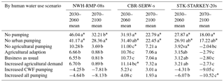
Streamflow predictions at two United States Geological Survey (USGS) gaging stations, the Hillsborough River (USGS ID: 02303330) and Alafia River (USGS ID: 02301500), were used in this study to evaluate retrospective and future IHM streamflow predictions and quantities of surface water available for public supply. Three Tampa Bay Water monitoring wells (NWH-RMP-08s, CBR-SERW-s, and STK-STARKEY-20s) were used to evaluate retrospective and future groundwater level predictions and compliance with environmental regulations intended to protect nearby wetlands from dewatering as a result of consolidated well field pumping.

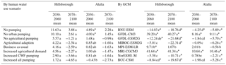
Table 1 Description of the CMIP5 models used in this study.

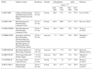
^* Change in precipitation (or ET₀) is defined as average of future period minus average of retrospective period.

2.3 Climate data

Forcing data from Phase 2 of the North American Land Data Assimilation System (NLDAS-2) from 1982 to 2005 were used as historical reference climate data for bias correction. Hourly precipitation, air temperature, solar radiation (surface downward longwave radiation and surface downward shortwave radiation), surface pressure, and average wind speed were obtained from the NLDAS-2 archive and aggregated to the daily scale at a 1∕8th-degree grid spacing over the Tampa Bay region.

For retrospective and future climate data, the Coupled Model Intercomparison Project 5 (CMIP5) GCM data set for the 1982–2005 period was used for the retrospective period, and 2030–2060 (future 1) and 2070–2100 (future 2) were used as future periods. Gridded daily precipitation, air temperature, solar radiation, surface pressure, and average wind speed were obtained for eight GCMs listed in Table 1. These GCMs were chosen because they spanned the range of cool to warm bias and wet to dry bias exhibited by 41 CMIP5 GCMs for the southeastern United States (Rupp, 2016), and they had daily values available for all the parameters needed to estimate Penman–Monteith reference evapotranspiration. Mean changes in precipitation projected by these GCMs ranged from −68 to 293 mm yr⁻¹ over the 2030–2060 period, and from 154 to 400 mm yr⁻¹ over the 2070–2100 period. Mean changes in ET₀ ranged from 24 to 137 mm yr⁻¹ over the 2030–2060 period and from 122 to 351 mm yr⁻¹ over the 2070–2100 period. Mean changes in P–ET₀ ranged from −162 to 220 mm yr⁻¹ over the 2030–2060 period and from −420 to 159 mm yr⁻¹ over the 2070–2100 period (Table 1).

S. Chang et al. (2016) evaluated projected changes in P–ET₀ over the continental USA using nine GCMs, 10 ET₀ estimation methods, and three RCP scenarios. They showed that the first-order sensitivities of water deficit projections (P–ET₀) over the southeastern USA were much higher to choice of GCM and ET₀ estimation method than to choice of RCP. First-order sensitivities of water deficit projections to RCP scenarios were negligible (<0.01) for the 2030–2060 time period, and averaged 0.2 for the 2070–2100 time period. Therefore for computational efficiency, and to evaluate the influence of the most extreme carbon dioxide forcing on the hydrologic projections, only the RCP 8.5 scenario data were utilized for the future analyses in this study.

2.4 BCSA downscaling method

The BCSA downscaling method, developed by Hwang and Graham (2013), was used in this study. Hwang and Graham (2014) showed that BCSA demonstrated better performance than other statistical downscaling methods (i.e., BCSD, Maurer and Hidalgo, 2008, or SDBC, Abatzoglou and Brown, 2012) in reproducing spatiotemporal statistics of both precipitation and daily streamflow in the Tampa Bay region. In particular, the INTB model, when driven by GCMs downscaled using the BCSA method, accurately reproduced frequencies of extreme high and extreme low retrospective streamflows as well as 7Q2 and 7Q10 retrospective streamflows in the Tampa Bay region.

The BCSA method preserves both the cumulative frequency distribution of observed daily precipitation as well as the spatial autocorrelation structure of observed daily precipitation fields. BCSA downscaling consists of two separate steps for bias correction and stochastic analog spatial downscaling. In the first step, a cumulative distribution function (CDF) mapping approach (Block et al., 2009; Hwang et al., 2013, 2014; Hwang and Graham, 2014; Ines and Hansen, 2006; Teutschbein and Seibert, 2012) is used to reduce the biases in raw GCM output at the GCM scale. In this study, NLDAS-2 P and ET₀ were aggregated up to the GCM scale and P and ET₀ from the raw GCMs were bias-corrected at the GCM scale using the sequential univariate CDF mapping method (Chang, 2017). NLDAS-2 was selected for bias correction because it includes all the parameters needed to estimate Penman–Monteith reference evapotranspiration. Comparison of the gridded NLDAS-2 data to the precipitation and temperature observations from the weather stations used to calibrate the INTB model showed that the NLDAS-2 data reproduced observed long-term monthly mean values with biases that ranged from 4 to 12 mm for daily precipitation and 1 to 2 ^∘C for daily temperature. Correlations among daily values ranged from 0.75 to 0.87 for rainfall and 0.75 to 0.98 for temperature. The second step in the BCSA method is stochastic analog (SA) spatial downscaling (Hwang and Graham, 2013, 2014) for P. In this method, a synthetic downscaled precipitation field is produced which preserves the GCM-scale daily precipitation amount and the month-specific local-scale spatial correlation structure. For more details on the BCSA method, see Hwang and Graham (2013, 2014). ET₀ was not downscaled in this study because observed spatial variability of ET₀ over the INTB region is very small, and the spatial correlation is large compared to P (Chang, 2017).

2.5 Reference evapotranspiration estimation methods

The S. Chang et al. (2016) study referenced above found that the projected changes in P–ET₀ were sensitive to both the choice of GCM and the choice of ET₀ method, and that for the southeastern USA the choice of GCM and ET₀ method had approximately equal influence on changes in future P–ET₀ throughout most of the year. However, they noted that not all 10 ET₀ methods were equally appropriate for use in all US regions, and that regional studies should use methods for which retrospective predictions of ET₀ are generally consistent with historic observations. Several of the ET₀ methods used by S. Chang et al. (2016) were found to produce unreasonably high or low historic ET₀ estimates for the study region using retrospective and observation data. Therefore in this study three ET₀ estimation methods that are widely used in the southeastern USA produced retrospective predictions that were consistent with observations, and showed that a range of wet to fairly dry projections of future P–ET₀ (S. Chang et al., 2016) were included in the analysis. These methods include a temperature-based method (Hargreaves; Hargreaves and Allen, 2003), a radiation-based method (Priestley–Taylor; Allen et al., 1998), and a combination method (Penman–Monteith; Allen et al., 1998). All hourly climate variables described above were aggregated to the daily scale and used to calculate daily ET₀ using these three methods.

2.6 Retrospective simulations

Water use in the study region is comprised of five categories: (1) public supply, (2) agricultural, (3) industrial/commercial, (4) mining, and (5) recreational (e.g., golf course irrigation) (Geurink and Basso, 2013). Groundwater sources are used for agricultural, industrial/commercial, mining, and recreational water supplies. Public water supply is provided by a combination of groundwater, surface water (Hillsborough and Alafia rivers), and a 25 MGD desalinization plant operated by Tampa Bay Water. The SWFWMD regulates all groundwater pumping and surface water extraction in the study region to protect natural aquatic ecosystems and prevent saltwater intrusion. Over the 1989–2006 calibration–verification period groundwater extractions from the INTB model domain averaged 36 mm yr⁻¹ for public water supply, 18 mm yr⁻¹ for agricultural irrigation, 9 mm yr⁻¹ for industrial/commercial uses, 6 mm yr⁻¹ for mining, and 3 mm yr⁻¹ for recreational uses (Geurink and Basso, 2013).

Public water supply. Tampa Bay Water has a consolidated permit for its 11 well fields (the Consolidated Wellfields, hereafter referred to as the CWFs). The CWFs are operated as an interconnected system with a combined maximum permitted pumping rate of 90 MGD (13 mm yr⁻¹ over the INTB region). Individual well pumping rates are optimized to maintain minimum groundwater levels near sensitive wetlands to meet regulatory requirements intended to prevent ecological harm. The three monitoring wells evaluated in this study are located near wetlands adjacent to the CWFs (Fig. 1). From 1992 to 2008 Tampa Bay Water's total water demand average ranged from 150 to 200 MGD. Groundwater is Tampa Bay Water's most inexpensive source of public water supply; therefore, for the retrospective simulations the CWFs were assumed to withdraw groundwater continuously at the 90 MGD maximum permitted rate. For the retrospective simulations groundwater extraction for other public water supply (outside of Tampa Bay Water's CWF), and industrial/commercial and mining uses, were assumed occur continuously at the average pumping rates between years 1989 and 2006 cited above.

Maximum surface water available to Tampa Bay Water for public supply was calculated on a daily basis from retrospective streamflow predictions for both the Hillsborough River and the Alafia River according to site-specific regulations set to maintain sufficient in-stream flows and spring flows to protect aquatic ecosystems. Diversion rates for pumping from the Hillsborough River reservoir by the City of Tampa and from the Tampa Bypass Canal by SWFWMD were set at the historical average daily rate spanning 2003 to 2009 for all retrospective simulations. All other diversion rates were set to zero, including the Withlacoochee–Hillsborough overflow. These diversion locations are located either downstream or outside of the watersheds contributing to the surface water gages, and outside the zone of influence of the monitoring wells evaluated in this study, so these assumptions do not impact on the results (Fig. 1).

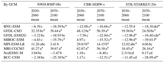
Table 2 Future scenario summary.

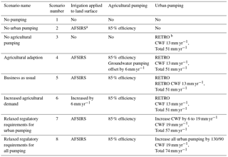
^a AFSIRS: climate-driven irrigation water demand estimated by the AFSIRS model using GCMs. ^b RETRO: groundwater pumping in the future will be equal to retrospective groundwater pumping.

Agricultural irrigation demand. The AFSIRS (Agricultural Field-Scale Irrigation Requirements Simulation) model (Jacobs and Dukes, 2007; Smajstrla, 1990) was used to estimate climate-driven irrigation demand for the retrospective period. The AFSIRS model tracks the water budget in the crop root zone including inputs from rain and irrigation, and outputs from the root zone by drainage and evapotranspiration. The AFSIRS model defines the water storage capacity in the crop root zone as the product of the water-holding capacity of the soil (estimated by the difference between field capacity and wilting point) and the depth of the effective root zone for the crop being grown. Crop evapotranspiration (ETc) is estimated from the product of potential evapotranspiration (ET₀) and crop water use coefficients. The AFSIRS model subdivides the crop root zone into irrigated and non-irrigated zones and maintains separate water budgets for both zones in order to simulate different types of irrigation systems, such as surface irrigation and subsurface irrigation.

The AFSIRS was used as a basis to estimate irrigation demand for the retrospective period using CMIP5 bias-corrected downscaled daily P and bias-corrected ET₀ (using the three ET₀ methods discussed above) and the land use from the calibrated INTB model. Crop coefficients (K_c) for estimating ET_c were obtained from the calibrated INTB model database (Geurink and Basso, 2013) for all vegetative covers except row crops. The crop coefficient for row crops was estimated by the superposition of crop coefficients for tomato and strawberry (Dukes et al., 2012), the two dominant row crops in the region. The relative proportion of these two crops constituting the row crop land use were calculated based on water usage records for the region for 2011 (Jackson and Albritton, 2013). The root zone depth, field capacity, wilting point, and other information needed for the AFSIRS model were taken from the calibrated INTB model database. Groundwater pumping required to satisfy the AFSIRS estimated irrigation assumed 85 % irrigation efficiency based on Irmak et al. (2011) and Jacobs and Dukes (2007), i.e.,

$$\begin{array}{}\text{(1)}& {\displaystyle }\text{agricultural pumping}=\text{irrigation demand}\times {\displaystyle \frac{\mathrm{100}\mathit{\%}}{\mathrm{85}\mathit{\%}}}.\end{array}$$

It should be noted that the AFSIRS model does not predict water demand for bed preparation, freeze protection, crop cooling requirements, or maintenance of irrigation systems. Thus the irrigation demand estimated for the retrospective period only includes crop water demand for evapotranspiration.

Boundary conditions. Lateral boundary conditions are required for aquifers in the model region. A repeating annual cycle of daily General Head Boundary (GHB) time series for the retrospective and future period IHM simulations was derived using the daily average of the historical daily GHB time series spanning 2000 to 2006. More details about the water withdrawals such as groundwater pumping, agricultural irrigation, CWFs, diversions, and boundary conditions during the calibration–verification period are described in Geurink and Basso (2013).

2.7 Future water use scenarios

In addition to warming temperatures and reduced precipitation due to climate change, increases in water withdrawal for agriculture and other human uses are potentially significant causes of declining river flow and groundwater levels (Alcamo et al., 2003; Vorosmarty et al., 2000). To assess the relative importance of climate change versus anthropogenic impact on the hydrologic system, ability to meet future water demand, and compliance with water resource regulations in the study region, eight future water use scenarios were developed (Table 2). These scenarios were based on discussions with Tampa Bay Water staff, projected increases in public water demand (Tampa Bay Water, 2013), projected changes in agricultural land use and agricultural irrigation demand (Florida Statewide Agricultural Irrigation Demand, 2017), potential agricultural adaption behaviors, and potential changes in groundwater regulations. For naming simplicity in the future scenarios agricultural and recreational water use categories are combined as agricultural demand and public supply; industrial/commercial and mining are combined as urban demand. The eight water use scenarios included (1) no groundwater pumping for agriculture or urban demand, (2) no urban groundwater pumping, (3) no agricultural groundwater pumping, (4) agricultural adaption (increased irrigation efficiency and/or use of reclaimed water), (5) business as usual, (6) increased agricultural demand, (7) relaxed regulatory requirements for CWF pumping (increased CWF pumping), and (8) relaxed regulatory requirements for all urban groundwater pumping (increased all urban pumping). Details regarding each of these water use scenarios are provided below.

The business as usual scenario (scenario 5 in Table 1) assumed no change in groundwater regulations. Thus the CWF pumping remained at the maximum permitted 90 MGD and all other urban pumping (industrial/commercial, mining, and other public water supply) remained at the average pumping rates used in the retrospective simulations. In this case all projected increases in future public water demand must be met by increased surface water extraction (if available), increased conservation, increased wastewater reuse, or desalination capacity. For the business as usual scenario agricultural irrigation demand was estimated using the AFSIRS model and assuming 85 % irrigation efficiency, as in the retrospective period simulations. However, the P and ET₀ used in the AFSIRS model were taken from the bias-corrected downscaled future GCM projections for both future 1 (2030–2060) and future 2 (2070–2100).

To more clearly separate the impact of human water use versus climate change on the hydrologic system, three extreme groundwater use reduction scenarios were developed. The no agricultural or urban pumping scenario (scenario 1) assumed that there was no groundwater pumping at all in the region. For this scenario agricultural and recreational pumping (and the associated irrigation of the land surface) as well as all urban pumping (including CWF, other public water supply, and industrial/mining) were set to zero. For the no urban pumping scenario (scenario 2) all urban pumping including CWF, other public water supplies, and industrial/mining was set to zero; however, agricultural pumping was assumed to be the same as the business as usual scenario. For the no agricultural pumping scenario (scenario 3) agricultural pumping and recreational pumping were set to zero; however, all urban pumping was assumed equal to the business as usual scenario.

The agricultural adaption scenario (scenario 4) assumed that increased irrigation efficiency and/or increased use of reclaimed water reduced groundwater pumping for agricultural and recreational irrigation by 40 MGD over climate-driven demand (6 mm yr⁻¹, ∼25 %). All urban pumping was assumed to be the same as the business as usual scenario. The increased agricultural demand scenario (scenario 6) assumed that irrigation demand increased by 40 MGD over climate-driven demand (6 mm yr⁻¹, ∼25 %) due to more intensive farming on existing agricultural lands (Florida Statewide Agricultural Irrigation Demand, 2017) and that all urban pumping was the same as the business as usual scenario. The relaxed regulatory requirements for CWF pumping (scenario 7) assumed an increase in CWF pumping up to 130 MGD (19 mm yr⁻¹, ∼44 %) from the current 90 MGD (13 mm yr⁻¹) to help meet increased public water demand, and that agricultural and recreational pumping followed the business as usual scenario. The relaxed regulatory requirements for all urban pumping (scenario 8) assumed all urban pumping, including CWF pumping, other public water supply, industrial, and mining, increased by 44 % (i.e., the same percentage increase as the CWF pumping for scenario 7) and that agricultural and recreational pumping followed the business as usual scenario. These water use scenarios consist of projected agricultural and urban groundwater pumping volumes that represent 0 % to 27 % of historic P–ET₀.

It should be noted that land use change was not considered in this study. This assumption is consistent with a regional planning strategy that promotes agricultural and urban intensification on existing lands, along with protection of existing conservation lands, wetlands and water supplies (Barnett et al., 2007). This assumption is also consistent with the Florida Statewide Agricultural Irrigation Demand (2017) that projects a 2 % decline in agricultural land area between 2015 and 2040, but an 8.5 % increase in agricultural water use as a net result of agricultural intensification and increased conservation. Future work will build on this study to evaluate land use change scenarios.

Table 3 The first-order sensitivity index of change in streamflow (future–retrospective period).

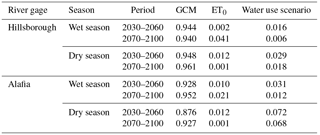
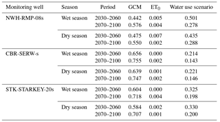
Table 4 The first-order sensitivity index of change in groundwater level (future–retrospective period).

2.8 Statistical analysis

Variance-based sensitivity analysis is a global sensitivity analysis (GSA) method (Saltelli et al., 2008, 2010) used to apportion the total model output variance simultaneously onto all the varying input factors, and thus is preferred over the local, one factor at a time, sensitivity analyses (Homma and Saltelli, 1996; Saltelli, 1999). In this research the sensitivity of projected changes between future and retrospective mean monthly streamflow and groundwater levels was evaluated using the variance-based GSA method described in S. Chang et al. (2016).

Using the variance-based GSA method, the variance-based first-order effect is expressed as

$$\begin{array}{}\text{(2)}& {\displaystyle }{V}_{X_i}\left(E_{X_{\sim i}}\left(Y\mathrm{|}{X}_i\right)\right),\end{array}$$

where V is the scalar model output (i.e., change in mean monthly streamflow or groundwater level), and X_i are the factors causing variation in the model output (i.e., choice of GCM, ET₀ method, and water use scenario). The expectation operator $E_{X_{\sim i}}\left(Y\mathrm{|}{X}_i\right)$ indicates that the mean of Y is taken over all possible values of X except X_i (i.e., X_∼ i) while keeping X_i fixed. The variance, $V_{X_i}$, is then taken of this quantity over all possible values of X_i. The first-order sensitivity coefficient is

$$\begin{array}{}\text{(3)}& {\displaystyle }{S}_i={\displaystyle \frac{V_{X_i}\left(E_{X_{\sim i}}\left(Y\mathrm{|}X\right)\right)}{V\left(Y\right)}},\end{array}$$

where V(Y) is the total variance of Y over all X_i. S_i is a normalized index varying between 0 and 1, because $V_{X_i}\left(E_{X_{\sim i}}\left(Y\mathrm{|}{X}_i\right)\right)$ varies between 0 and V(Y) according to the identity (Mood et al., 1974):

$$\begin{array}{}\text{(4)}& {\displaystyle }{V}_{X_i}\left(E_{X_{\sim i}}\left(Y\mathrm{|}{X}_i\right)\right)+E_{X_i}\left(V_{X_{\sim i}}\left(Y\mathrm{|}{X}_i\right)\right)=V\left(Y\right).\end{array}$$

The first-order sensitivities of future changes in mean seasonal streamflow and groundwater level to the choice of GCM, ET₀ estimation method, and water use scenario were calculated over the full ensemble of eight GCMs, three ET₀ methods, and eight water use scenarios (192 samples) for each future period in order to evaluate the relative contributions of each of these factors to the variation among projections of future changes.

In addition to variance-based GSA, differences in future changes of mean projected streamflow and groundwater level across GCMs and across future water use scenarios were evaluated for statistical significance using Tukey's HSD (honest significant difference) test (Zieyel, 1988), which is a single-step multiple statistical test (pairwise comparison). The two-sample t test was used to test for significant differences between mean projected streamflow and groundwater levels resulting from future climate/water use scenarios and mean retrospective streamflow and groundwater level using the business as usual water use scenario.

3 Results and discussion

3.1 Global sensitivity analysis of projected changes

The variance-based global sensitivity analysis was conducted for both the wet season (June–September) and the dry season (October–May) to evaluate the relative variation of projected changes in hydrologic response attributed to the choice of GCM, choice of water use scenario, and choice of ET₀ method. Tables 3 and 4 show the first-order sensitivity indices of changes in future streamflow and groundwater level (defined as future average seasonal streamflow, retrospective average seasonal streamflow and future average seasonal groundwater level, and retrospective average seasonal groundwater level, respectively).

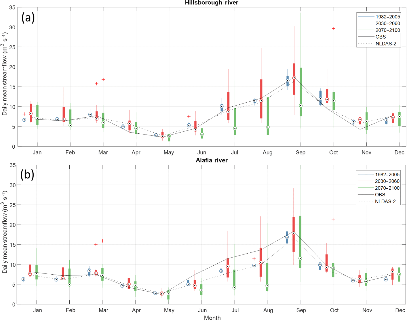
Figure 2 Mean monthly streamflow for the Hillsborough River (a) and Alafia River (b) for business as usual scenario water use and the Hargreaves ET₀ method. Boxplots indicate the range of prediction over the eight GCMs.

Change in streamflow was much more sensitive to choice of GCM than to choice of ET₀ method or water use scenario for all river gages, both seasons, and both future periods (Table 3). For example, 94.4 % of the variance of the change in wet season Hillsborough River streamflow in the future 1 period (2030–2060) is attributed to differences among GCMs, 0.2 % of the variance is attributed to differences among the ET₀ method, and 1.6 % of the variance is caused by the water use scenario, respectively (top row of Table 3). Similarly, projected changes in groundwater level were generally more sensitive to the choice of GCM for all monitoring wells and both seasons. However, unlike the projected changes in streamflow, changes in groundwater level were also quite sensitive to the choice of water use scenario (Table 4). The higher sensitivity of groundwater level to groundwater pumping is expected since the monitoring wells are intentionally located near the consolidated well fields (locations of major groundwater pumping) to detect and mitigate localized impacts of water supply pumping on nearby wetlands. On the other hand, the stream gages are located further from the consolidated well fields and accumulate flow from a large area of the model domain. The first-order sensitivity index of groundwater level to water use scenario decreased in future period 2 (2070–2100) over future period 1 (2030–2060), due to the increased variability of GCM precipitation projections in future 2 (2070–2100) versus future 1 (2030–2060).

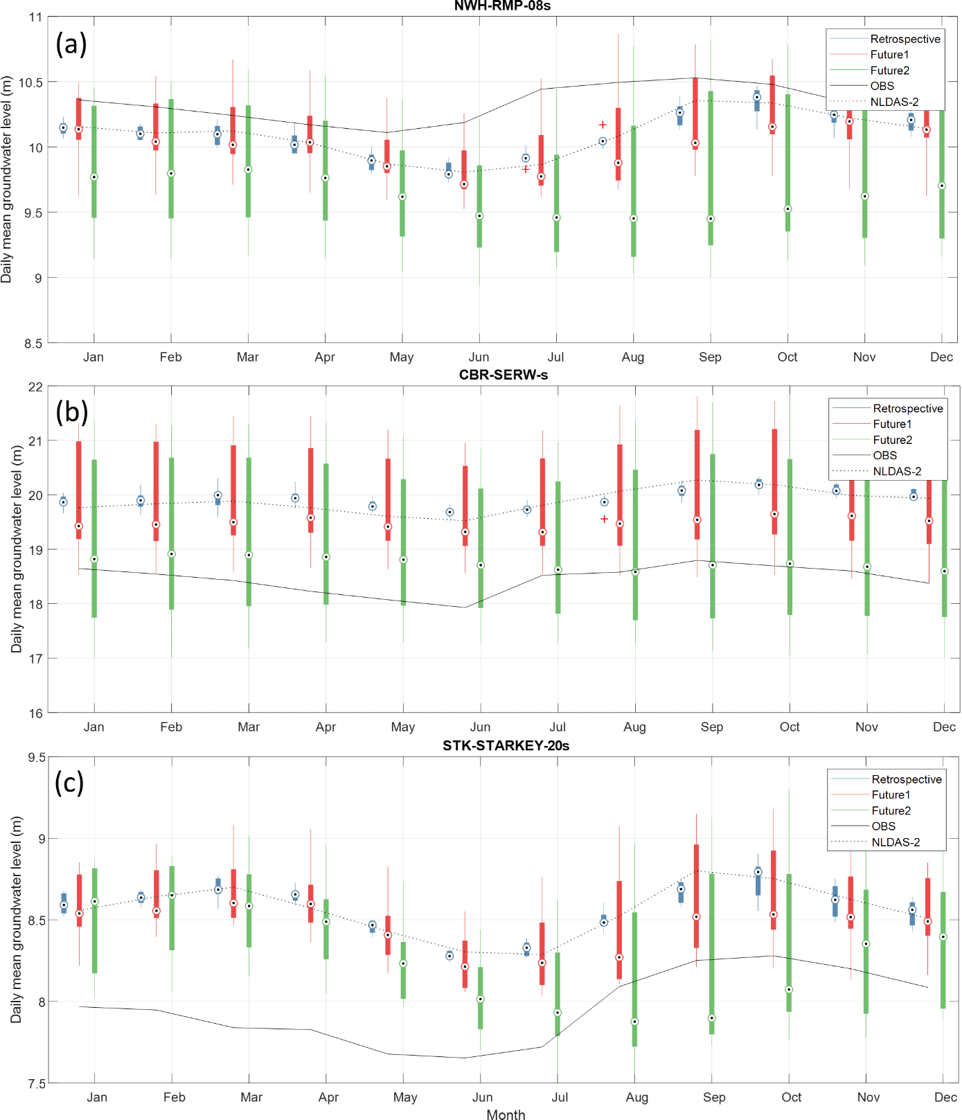
Figure 3 Mean monthly groundwater level for the NWH-RMP-08s (a), CBR-SERW-s (b) and STK-STARKEY-20s (c) for the business as usual water use scenario and the Hargreaves ET₀ method. Boxplots indicate the range of prediction over the eight GCMs.

As mentioned previously, S. Chang et al. (2016) evaluated projected changes in P–ET₀ over the continental USA using nine GCMs, 10 ET₀ estimation methods, and three RCP scenarios, and found that for the southeastern USA the choice of GCM and ET₀ method had approximately equal influence on changes in future P–ET₀ throughout most of the year. Because this study eliminated several ET₀ estimation methods that produced unreasonably high and low historic ET₀ estimates for the study region using the NLDAS-2 data, the first-order sensitivity index for ET₀ is significantly lower in this study than in their results. It should be noted that these results do not indicate that the choice of reference ET estimation method does not affect the change in streamflow or groundwater, only that the choice of reference ET estimation method is much less influential than the choice of GCM or choice of water use scenario.

3.2 Projections of streamflow

The INTB was run to compare retrospective hydrologic response to historical observations and model predictions generated with the calibrated model using NLDAS-2 data, as well as to future hydrologic response as a result of alternative GCMs, ET₀ methods, and water use scenarios. Figure 2 shows observed, NLDAS-2, and retrospective mean monthly streamflow for the Hillsborough River (Fig. 2a) and Alafia River (Fig. 2b), as well as future mean monthly streamflow in future 1 (2030–2060) and future 2 (2070–2100) for the business as usual water use scenario using the Hargreaves ET₀ method originally used to calibrate the INTB model. The boxplots represent the range of mean monthly streamflow projections over eight GCMs for the business as usual water use scenario. Retrospective GCMs (blue boxplots) reproduced mean streamflow simulated using NLDAS-2 data quite closely for both river gages, with relatively small variation among GCMs. In the dry season (October–May) future 1 (red boxplots) and future 2 (green boxplots) business as usual mean monthly streamflow values over the eight GCMs (red boxplots) also showed relatively small differences with the retrospective predictions, but larger variation across GCMs. However, in the wet season (June through September) future mean monthly streamflows for the business as usual scenario were lower than retrospective, especially in future 2 (2070–2100), and showed much larger variability across GCMs.

Figure 4 The change in the amount of available water that can be withdrawn from the Hillsborough River by (a) different water use scenarios over GCM and ET₀ methods and by (b) different GCMs over water use scenarios and ET₀ methods.

3.3 Projections of groundwater level

Figure 3 shows observed, NLDAS-2 predicted, and retrospective mean monthly groundwater level for the NWH-RMP-08s (Fig. 3a), CBR-SERW-s (Fig. 3b), and STK-STARKEY-20s wells (Fig. 3c), as well as future mean monthly groundwater level in future 1 (2030–2060) and future 2 (2070–2100) for the business as usual water use scenario and the Hargreaves ET₀ method. Groundwater levels projected by retrospective GCMs showed relatively small variation across GCMs and were very similar to groundwater levels simulated using the historic NLDAS-2 data for all three wells. Although observed seasonal patterns were reproduced accurately for all wells during the retrospective period, NWH-RMP-08s retrospective groundwater level predictions were lower than observed groundwater levels throughout the year (Fig. 3a). In contrast, all CBR-SERW-s and STK-STARKEY-20s retrospective groundwater lever predictions were higher than observed groundwater levels throughout the year (Fig. 3b and c). These deviations (which are generally less than 0.5 m) are consistent with deviations between the observed data and groundwater levels simulated by the original calibrated model using the locally observed point weather data (Geurink and Basso, 2013). The mean groundwater levels averaged over GCMs for the future period 1 (2030–2060) business as usual scenario were similar to, or slightly lower than, the mean retrospective groundwater levels; however, the mean groundwater levels for future 2 (2070–2100) were significantly lower than mean groundwater levels in the retrospective period, especially in the wet season for all wells. Similar to the streamflow results variability in projected groundwater levels among GCMs was larger in future 2 (2070–2100) than in future 1 (2030–2060).

3.4 Changes in future surface-water availability for public supply

Tampa Bay Water operates surface-water pumps on the Hillsborough and Alafia rivers to help meet public water demand. The volume of flow permitted for extraction varies daily based on maintaining sufficient in-stream flows and spring flows to protect aquatic ecosystems. In this study, the amount of water that could be withdrawn for public water supply, while meeting current environmental regulations, was analyzed to evaluate projected changes in future water availability for different GCMs and water use scenarios. Boxplots in Fig. 4a show the variation in the projected change in the mean available water that can be withdrawn from the Hillsborough River (the mean available water that can be withdrawn for future streamflow − the mean available water that can be withdrawn for retrospective streamflow) over all GCMs and all ET₀ methods for each water use scenario. The boxplots show large variations due to large differences in future streamflow projections. All boxplots encompass both positive and negative changes for both future periods, but indicate generally lower water availability in future 2 (2070–2100) than future 1 (2030–2060). Figure 4b compares the change in the projected mean available water that can be withdrawn from the Hillsborough River over water use scenarios and ET₀ methods for each GCM. While there is some variation across water use scenarios and ET₀ methods, Fig. 4b clearly shows that projected changes in future surface water availability depend strongly on choice of GCM, with five GCMs showing less surface water availability in the future regardless of water use scenario. Plots for the Alafia River show very similar behavior by both water use scenario and GCM (Fig. S1 in the Supplement).

Table 5 The results of Tukey's HSD test of mean change in the amount of available water (MGD) that can be withdrawn from the Hillsborough River or Alafia River for each water use scenario over GCM and ET₀ methods, or for each GCM over water use scenario and ET₀ method (comparison of all possible pairs of means).

Means with different subscripts were significantly different in Tukey's HSD test. ^* The results were significantly different than retrospective BAU by a two-sample t test at the 0.05 significance level.

The differences between the mean projected changes in available water that can be withdrawn from the Hillsborough and Alafia rivers for individual water use scenarios over GCMs and ET₀ methods (left columns in Table 5), and for individual GCMs over water use scenarios and ET₀ methods (right columns in Table 5), were evaluated for statistical significance using Tukey's HSD (honest significant difference) test. The HSD test confirmed that none of the differences in the mean projected change in available water for different water use scenarios shown in Fig. 3a were statistically significant for the Hillsborough River for either future period (in Table 5 scenarios with the same alphabetic subscripts are not statistically significantly different). For the Alafia River the mean projected changes in available water for the extreme groundwater pumping reduction scenario was statistically significantly different from the other water use scenarios in future 1 (2030–2060), but no statistically significant changes were detected in future 2 (2070–2100). These results imply that due to the large variations in climate projections produced by different GCMs, differences in mean projected changes in streamflow projections due to differences water use scenarios and ET₀ methods cannot be reliably predicted by averaging over GCMs.

On the other hand, many of the differences between mean projected changes in available water that can be withdrawn from the Hillsborough and Alafia rivers for individual GCMs over water use scenarios were statistically significant for both future periods (i.e., many of the GCMs on the right side of Table 5 have different alphabetic subscripts). Two GCMs show a distinct increase in water availability from these rivers for public supply (GFDL-CM3 and MRI-CGCM3); however, most GCMs show a decrease in water availability (BNU-ESM, GFDL-ESM2G, MIROC-ESM, NorESM1-M, and BCC-CSM). These results underscore the fact that differences in projections of future availability of water from these rivers for public supply are driven more strongly by differences in climate models than differences in future human water use scenarios or ET₀ methods. Furthermore, manipulating groundwater use to change the amount of available surface water has a very small effect for a given climate. These results are similar to previous studies (Bosshard et al., 2013; Forzieri et al., 2014; Guimberteau et al., 2013; Harding et al., 2012; Kay and Davies, 2008) that showed climate models are a large source of uncertainty for climate-impact projections because of the divergence of GCM projections.

In addition to the HSD test, the two-sample t test was conducted to evaluate the statistical significance of differences between the mean available water that can be withdrawn for the retrospective period and the mean available water that can be withdrawn for each future water use scenario calculated over all GCMs and ET₀ methods. The two-sample t test indicated that, at the 0.05 significance level, none of the future scenarios were statistically significantly different from the retrospective business as usual scenario for the Hillsborough River. For the Alafia River only the no pumping and no urban pumping scenarios in future 1 (2030–2060) showed significant differences from the retrospective scenario in the available water that can be withdrawn from the Alafia River (marked as ^* in the left-hand columns of Table 5). In contrast most GCMs projected significantly different mean available water in both future periods compared to the retrospective period when averaged over water use scenarios (marked as ^* in the right-hand columns of Table 5).

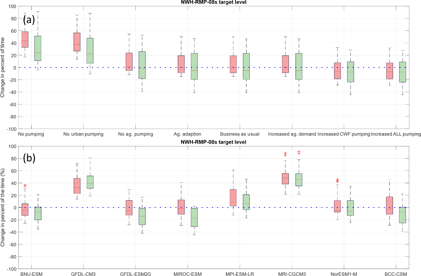
Figure 5 The change in the percent of the time that groundwater level is above the target level for NWH-RMP-08s well by (a) different water use scenarios over GCMs and ET₀ methods and by (b) different GCMs over water use scenarios and ET₀ methods.

The results that future streamflow projections are relatively insensitive to water use scenarios are contrary to that of Dale et al. (2015). They used historical streamflow and climate data to evaluate the impacts of anthropogenic change on streamflow and found that for an irrigation-intensive watershed located in an area with hot summers and limited precipitation (northern central Oklahoma, USA) irrigation from groundwater pumping increased antecedent soil moisture and played an equally important role in streamflow variability as climate change. These differences are likely due to that fact that the region studied here is wetter than their study region, the aquifer underlying the study region is large and productive, and land use changes were not considered in this study.

3.5 Changes in compliance with groundwater level regulations

Groundwater pumping for water supply in the Tampa Bay region is regulated to maintain groundwater levels that promote environmental protection by preventing dewatering of lakes and wetlands near well fields. The relative importance of water use scenario and GCM selection on the change in percent of time that future groundwater levels were above the target levels (the percent of the time that groundwater level is above the target level for future scenario – the percent of the time that groundwater level is above the target level for retrospective scenario) was evaluated for three monitoring wells. Boxplots in Fig. 5a show the change in percent of the time that groundwater level was above the target level in the dry season (October–May) for the NWH-RMP-08s well over all GCMs for each water use scenario and ET₀ methods. Tukey's HSD test showed that the two most extreme water use reduction scenarios, i.e., the no pumping scenario and the no urban pumping scenario, showed a statistically significant higher percent of time that groundwater is above the target level in future 1 (2030–2060) compared to the other future water use scenarios for the NWH-RMP-08s well (Table 6). Furthermore the t test showed a statistically significant difference in the percent of time this well was above the target level in both futures 1 (2030–2060) and 2 (2070–2100) for these two scenarios compared to the retrospective scenario (marked with ^* in Table 6). Results for the other two wells were more ambiguous with Tukey's HSD test showing differences among several of the water use scenarios in future 1 for both wells, and among several water use scenarios in future 2 for STK-STARKEY-20s. The t test for CBR-SERW-s and STK-STARKEY-20s showed statistically significant differences for the two most extreme water use reduction scenarios compared to the retrospective scenario both future 1 and future 2. Collectively these results confirm that future compliance with groundwater levels is sensitive to water use scenario. Scenarios that assume differences in CWF pumping predict statistically significant differences in future groundwater compliance when averaged over possible future climates and ET₀ methods. On the other hand scenarios that assume similar differences in the magnitude of agricultural pumping generally do not show statistically significant differences in future groundwater compliance. These results are largely explained by the concentration of CWF wells near monitoring wells versus the distribution of agricultural pumping wells throughout the model domain.

Table 6 The results of Tukey's HSD test of mean change in the percent of the time that groundwater level is above the target level for monitoring wells over all GCMs and ET₀ methods for each water use scenario (comparison of all possible pairs of means).

Means with different subscripts were significantly different in Tukey's HSD test. ^* The results were significantly different than retrospective BAU by a two-sample t test at the 0.05 significance level.

Table 7 The results of Tukey's HSD test of mean change in percent of the time that groundwater level is above the target level for monitoring wells over all water use scenarios and ET₀ methods for each GCM (comparison of all possible pairs of means).

Means with different subscripts were significantly different in Tukey's HSD test. ^* The results were significantly different than retrospective BAU by a two-sample t-test at the 0.05 significance level.

Figure 5b indicates and Tukey's HSD test (Table 7) confirms that the mean change in percent of time that groundwater is above the target level in the monitoring wells was significantly different for many GCMs in both future periods for all three wells (Figs. 5 and S2–S3). Two “wet” GCMs (GFDL-CM3 and MRI-CGCM3) projected statistically significant increases in the mean percent of the time that groundwater is above the target level for both future periods compared to the retrospective period in all three wells when averaged over future water use scenario and ET₀ method (Fig. 5b and marked as ^* in the Table 7). Three “drier” GCMs (BNU-ESM, MIROC-ESM and BCC-CSM) projected statistically significant decreases in percent of the time that groundwater level is above the target level compared to the retrospective period in future 2 (2070–2100) for all three wells. More GCMs showed significant differences in future period 2 (2070–2100) than in future period 1 (2030–2060) compared to the retrospective period because the differences among climate model projections increase in the later future. These results indicate that for drier future climate groundwater level regulations may be difficult to achieve regardless of groundwater pumping scenario, and thus may have to change with the changing climate.

3.6 Ability to meet future water demand

Future water demand projections for Tampa Bay Water indicate that even with active urban water conservation programs public water supply demand is expected to increase from approximately 220 MGD in 2010 to approximately 278 MGD in 2045 (Tampa Bay Water Water Demand Management Plan Final Report, 2013). At the present time the Tampa Bay water supply system includes 90 MGD groundwater pumping permitted for the CWF, a 25 MGD desalination plant and permitted water withdrawals from the Hillsborough and Alafia rivers that vary daily to maintain ecologically protective in-stream flows. Scenario discovery analysis (Tariq et al., 2017) was used to explore the ability of Tampa Bay Water to meet 2045 water demand while maintaining or improving existing levels of compliance with surface and groundwater regulations.

Figure 6 Scatterplot of futures in which Tampa Bay Water meets 2045 water demands and maintains or improves compliance with groundwater regulations in future 1 (2030–2060) assuming 0 %, 20 %, and 40 % of freshwater withdrawn are reclaimed and reused to satisfy urban demand. Green filled circles indicate futures that meet both 2045 water demand and maintain groundwater compliance levels at or above current conditions. Yellow filled circles indicate futures that meet 2045 water demand but decrease the level of groundwater compliance. Orange filled circles indicate futures that do not meet 2045 water demand but maintain groundwater compliance levels at or above current conditions. Red filled circles indicate futures that do not meet 2045 water demand and decrease the level of groundwater compliance. The black filled circle indicates the retrospective business as usual condition.

Figure 6 presents the results of the scenario discovery analyses that evaluates which climate and water use scenarios achieve these objectives in future 1 (2030–2060) using the Hargreaves ET₀ method. In these analyses it was assumed that Tampa Bay Water's desalination capacity would remain at 25 MGD, surface water would be extracted at the maximum rate that complied with existing regulations, and 0 % (current condition), 20 %, or 40 % of Tampa Bay Water's public water supply (surface water, groundwater, and desalination) might be reclaimed and reused to satisfy public demand. The axes in Fig. 6 represent the two most important factors in the climate and water use scenarios that affect achievement of Tampa Bay Water's goals: mean change in precipitation projected by the different GCMs and volume of agricultural and urban groundwater pumping in the water use scenario. Green filled circles indicate futures that meet both 2045 water demand and maintain groundwater compliance levels at or above current conditions in future 1 (2030–2060). Yellow filled circles indicate futures that meet 2045 water demand but decrease the level of groundwater compliance. Orange filled circles indicate futures that do not meet 2045 water demand but maintain groundwater compliance levels at or above current conditions. Red filled circles indicate futures that do not meet 2045 water demand and decrease the level of groundwater compliance. The black filled circle indicates the retrospective business as usual condition.

Figure 6a shows that, without using reclaimed water to satisfy public water demand, only four scenarios are able to meet 2045 demand and maintain or improve existing levels of compliance with groundwater regulations (filled green circles in Fig. 6a). These four scenarios assume the two wettest future climates (projected by GFDL-CM3 and MRI-CGM3) will occur and permitted CWF pumping will increase from 90 to 130 MGD. No other climate–water use scenarios are able to meet 2045 demand without use of reclaimed water (there are no yellow filled circles in Fig. 6a). In fact a significant number of the scenarios, including many that assume the business as usual water use scenario, are not able to meet 2045 demand and also decrease compliance groundwater regulations (red filled circles in Fig. 6a).

Figure 6b shows that 20 % of freshwater withdrawn is reclaimed and used to satisfy public demand the two wettest future climates can meet 2045 demand and maintain or improve existing levels of compliance with groundwater regulations for all water use scenarios. However, no other scenarios are able to achieve both goals. If 40 % of freshwater withdrawn is reclaimed and used to satisfy public demand more scenarios are able to achieve both goals. These scenarios include the climate scenarios that project that at least the existing average annual rainfall will occur in the future (i.e., projected change in average annual rainfall greater than or equal to zero). However, to meet both public water demand and maintain existing compliance with groundwater regulations, scenarios that predict the same rainfall as current climate require a complete switch of public water supply from groundwater to surface water sources (bottom two water use scenarios in Fig. 6). This would require Tampa Bay Water to significantly increase their surface water storage and treatment capacity and eliminates the use of their most inexpensive water source (groundwater). If groundwater regulations were relaxed, and 40 % freshwater withdrawn in reclaimed, 2045 demand could be met under any climate scenario (yellow circles in Fig. 6c). It should be noted that the Regional Water Supply Planning (2016) reported that in 2015 only about 11.5 % of total freshwater withdrawn was reused in Florida. Therefore reclaiming 20 %–40 % of freshwater withdrawn will be a significant investment.

4 Conclusions

It is important to evaluate possible changes in future streamflow and groundwater levels to evaluate risks in water resource management and planning. This study investigated potential future changes in hydrologic systems, ability to meet future water demand, and compliance with water resource regulation using eight GCMs, eight human water use scenarios, and three ET₀ methods to drive an integrated hydrologic model developed for the Tampa Bay region. Variance-based sensitivity analysis showed that changes in projected streamflow were very sensitive to GCM selection, but relatively insensitive to ET₀ method or water use scenario. Changes in projections of groundwater level were sensitive to both GCM and water use scenario, but relatively insensitive to ET₀ method.

The eight GCMs projected diverse changes in streamflow and groundwater level, with most GCMs projecting statistically significant different future streamflow and groundwater levels than the current condition. Five of the eight GCMs projected a decrease in future streamflow and groundwater level in the INTB region regardless of water use scenario or ET method. None of the eight GCMs projected that 2045 water demand could be met under the business as usual water use scenario. Two GCMs (GFDL-CM3 and MRI-CGCM3) predicted increased streamflow and groundwater levels and an ability to meet 2045 projected water demand and maintain existing levels of compliance with groundwater standards if permitted CWF pumping were increased from the current 90 MGD to 130 MGD. The GCM that predicted that future annual average rainfall will be approximately equal to current rainfall met 2045 demand maintained existing levels of compliance with groundwater standards only for the water use scenarios that eliminated CWF pumping completely and reclaimed 40 % of freshwater withdrawals.

These results suggest that it is more likely than not that climate change will reduce the availability of both surface and groundwater for public supply in the Tampa Bay region. Current regulations on water withdrawals (surface water withdrawal permit thresholds and target levels in monitoring wells near lakes and wetlands) may have to adapt to future climate conditions since only extreme changes in human water use (i.e., dramatic increases in use of reclaimed water and a complete switch from groundwater to surface water) may be able to maintain retrospective hydrologic regimes and associated aquatic ecosystems and meet human water demand in the future.

It should be noted that the findings of this study are limited by a few major assumptions. For example this study used only eight GCMs to project future climate which is a relatively small number. However, these eight GCMs spanned the range of cool to warm bias and wet to dry bias exhibited by 41 CMIP5 GCMs for the southeastern United States (Rupp, 2016). In addition land use change was not considered in this study. Instead we assumed the increases in agricultural and urban water demand were the result of intensification of water use on existing land uses. This assumption is consistent with a regional planning strategy that promotes agricultural and urban intensification on existing lands, along with protection of existing conservation lands, wetlands and water supplies (Barnett et al., 2007). However, future work should build on this study to evaluate the additional impacts of potential land use change scenarios (Gupta et al., 2015; Lin et al., 2015; Matheussen et al., 2000; Yan et al., 2013).