Nitrogen attenuation, dilution and recycling in the intertidal hyporheic zone of a subtropical estuary

Tidal estuarine channels have complex and dynamic interfaces controlled by upland groundwater discharge, waves, tides and channel velocities that also control biogeochemical processes within adjacent sediments. In an Australian subtropical estuary, discharging groundwater with elevated (> 300 mg N L⁻¹) ${\mathrm{NH}}_{\mathrm{4}}^{+}$ and ${\mathrm{NO}}_{\mathrm{3}}^{-}$ concentrations had 80 % of the N attenuated at this interface, one of the highest N removal rates (> 100 mmol m⁻² day⁻¹) measured for intertidal sediments. The remaining N was also diluted by a factor of 2 or more by mixing with surface water before being discharged to the estuary. Most of the mixing occurred in a hyporheic zone in the upper 50 cm of the channel bed. However, groundwater entering this zone was already partially mixed (12 %–60 %) with surface water via tide-induced circulation. Below the hyporheic zone (50–125 cm below the channel bed), ${\mathrm{NO}}_{\mathrm{3}}^{-}$ concentrations declined slightly faster than ${\mathrm{NH}}_{\mathrm{4}}^{+}$ concentrations and δ${}^{\mathrm{15}}{\mathrm{N}}_{{\mathrm{NO}}_{\mathrm{3}}}$ and δ${}^{\mathrm{18}}{\mathrm{O}}_{{\mathrm{NO}}_{\mathrm{3}}}$ gradually increased, suggesting a co-occurrence of anammox and denitrification. In the hyporheic zone, δ${}^{\mathrm{15}}{\mathrm{N}}_{{\mathrm{NO}}_{\mathrm{3}}}$ continued to become enriched (consistent with either denitrification or anammox) but δ${}^{\mathrm{18}}{\mathrm{O}}_{{\mathrm{NO}}_{\mathrm{3}}}$ became more depleted (indicating some nitrification). A high δ${}^{\mathrm{15}}{\mathrm{N}}_{{\mathrm{NO}}_{\mathrm{3}}}$ (23 ‰–35 ‰) and a low δ${}^{\mathrm{18}}{\mathrm{O}}_{{\mathrm{NO}}_{\mathrm{3}}}$ (1.2 ‰–8.2 ‰) in all porewater samples indicated that the original synthetic nitrate pool (industrial NH₄NO₃; δ¹⁵N ∼ 0 ‰; δ¹⁸O ∼ 18 ‰–20 ‰) had turned over completely during transport in the aquifer before reaching the channel bed. Whilst porewater ${\mathrm{NO}}_{\mathrm{3}}^{-}$ was more δ¹⁸O depleted than its synthetic source, porewater δ${}^{\mathrm{18}}{\mathrm{O}}_{{\mathrm{H}}_{\mathrm{2}}\mathrm{O}}$ (−3.2 ‰ to −1.8 ‰) was enriched by 1 ‰–4 ‰ relative to rainfall-derived groundwater mixed with seawater. Isotopic fractionation from H₂O uptake during the N cycle and H₂O production during synthetic ${\mathrm{NO}}_{\mathrm{3}}^{-}$ reduction are the probable causes for this δ${}^{\mathrm{18}}{\mathrm{O}}_{{\mathrm{H}}_{\mathrm{2}}\mathrm{O}}$ enrichment. Whilst occurring at a smaller spatial scale than tide-induced circulation, hyporheic exchange can provide a similar magnitude of mixing and biogeochemical transformations for groundwater solutes discharging through intertidal zones.

1 Introduction

In permeable sediments, there is active mixing between surface water and groundwater by hyporheic exchange and seawater recirculation (Jones and Mulholland, 2000; Heiss and Michael, 2014) (Fig. 1). Hyporheic exchange is induced by flows and currents over uneven riverbeds creating zones where surface water moves in and porewater moves out of the sediments (Harvey and Bencala, 1993). In marine environments, tides, wave action and density differences between discharging fresh groundwater and seawater also generate groundwater–surface-water mixing (collectively referred to here as seawater recirculation) (Burnett et al., 2003; Sawyer et al., 2013; Precht and Huettel, 2003; Pool et al., 2015). When concentrations are more elevated in groundwater, hyporheic exchange and seawater recirculation can spread a solute load over time and in general will tend to lower concentrations at the discharge point (Li et al., 1999; Murgulet and Tick, 2016). However, because hyporheic exchange and seawater recirculation also bring labile organic matter, oxygen and other compounds to the subsurface (Santos et al., 2011; Ahmerkamp et al., 2017), mixing zones are also very active biogeochemical environments where reactive contaminants like ${\mathrm{NH}}_{\mathrm{4}}^{+}$ and ${\mathrm{NO}}_{\mathrm{3}}^{-}$ can be attenuated via a range of biogeochemical processes (Ullman et al., 2003; Abe et al., 2009; Ueda et al., 2003). When attenuation also takes place, both the contaminant concentration and the contaminant load to surface water is reduced by groundwater–surface-water exchange.

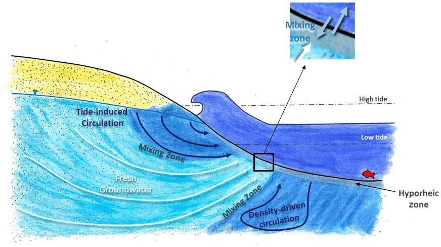
Figure 1 Conceptual representation of the different scales of groundwater–surface-water mixing in the intertidal zone (modified from Heiss and Michael, 2014).

The mixing and attenuation of ${\mathrm{NH}}_{\mathrm{4}}^{+}$ and ${\mathrm{NO}}_{\mathrm{3}}^{-}$ in contaminated groundwater discharging into a subtropical southeast Australian estuary was evaluated by collecting channel bed porewater profiles using a drive point (Cranswick et al., 2014). Chloride was used as a conservative tracer to determine the effect of movement and mixing; ²²²Rn estimated residence times (Hoehn and Cirpka, 2006; Lamontagne and Cook, 2007) and various other parameters (including ${\mathrm{NH}}_{\mathrm{4}}^{+}$ and ${\mathrm{NO}}_{\mathrm{3}}^{-}$ concentrations and the dual isotopes of ${\mathrm{NO}}_{\mathrm{3}}^{-}$) evaluated N cycling in the subsurface. The isotopic composition of water was also initially measured to evaluate mixing owing to the large difference in isotopic composition between rainfall-derived groundwater and seawater (Clark and Fritz, 1997). However, the isotopic composition of groundwater was found not to be conservative and was used to further evaluate N attenuation processes. For proprietary reasons, details on the exact location of the site are not being reported.

1.1 Key biogeochemical processes

In a contaminated aquifer environment, some of the key processes likely to control the N cycle will include nitrification (Casciotti et al., 2010),

$$\begin{array}{}\text{(1)}& {\displaystyle }{\mathrm{NH}}_{\mathrm{4}}^{+}+\mathrm{2}{\mathrm{O}}_{\mathrm{2}}\to {\mathrm{NO}}_{\mathrm{3}}^{-}+{\mathrm{H}}_{\mathrm{2}}\mathrm{O}+\mathrm{2}{\mathrm{H}}^{+};\end{array}$$

denitrification (here shown via organic matter oxidation; Schiff and Anderson, 1987),

$$\begin{array}{ll}{\displaystyle }& {\displaystyle }{\left({\mathrm{CH}}_{\mathrm{2}}\mathrm{O}\right)}_{\mathrm{106}}{\left({\mathrm{NH}}_{\mathrm{3}}\right)}_{\mathrm{16}}\left({\mathrm{H}}_{\mathrm{3}}{\mathrm{PO}}_{\mathrm{4}}\right)+\mathrm{94.4}{\mathrm{NO}}_{\mathrm{3}}^{-}+\mathrm{92.4}{\mathrm{H}}^{+}\\ \text{(2)}& {\displaystyle }& {\displaystyle }\to \mathrm{106}{\mathrm{CO}}_{\mathrm{2}}+\mathrm{55.2}{\mathrm{N}}_{\mathrm{2}}+{\mathrm{HPO}}_{\mathrm{4}}^{-\mathrm{2}}+\mathrm{177.2}{\mathrm{H}}_{\mathrm{2}}\mathrm{O};\end{array}$$

dissimilatory ${\mathrm{NO}}_{\mathrm{3}}^{-}$ reduction to ${\mathrm{NH}}_{\mathrm{4}}^{+}$ (DNRA, here shown via organic matter oxidation; Schiff and Anderson, 1987),

$$\begin{array}{ll}{\displaystyle }& {\displaystyle }{\left({\mathrm{CH}}_{\mathrm{2}}\mathrm{O}\right)}_{\mathrm{106}}{\left({\mathrm{NH}}_{\mathrm{3}}\right)}_{\mathrm{16}}\left({\mathrm{H}}_{\mathrm{3}}{\mathrm{PO}}_{\mathrm{4}}\right)+\mathrm{53}{\mathrm{NO}}_{\mathrm{3}}^{-}+\mathrm{120}{\mathrm{H}}^{+}\\ \text{(3)}& {\displaystyle }& {\displaystyle }\to \mathrm{106}{\mathrm{CO}}_{\mathrm{2}}+\mathrm{69}{\mathrm{NH}}_{\mathrm{4}}^{+}+{\mathrm{HPO}}_{\mathrm{4}}^{-\mathrm{2}}+\mathrm{53}{\mathrm{H}}_{\mathrm{2}}\mathrm{O};\end{array}$$

and anaerobic ammonium oxidation (anammox; Brunner et al., 2013),

$$\begin{array}{}\text{(4)}& {\displaystyle }\mathrm{1.3}{\mathrm{NO}}_{\mathrm{2}}^{-}+{\mathrm{NH}}_{\mathrm{4}}^{+}\to {\mathrm{N}}_{\mathrm{2}}+\mathrm{0.3}{\mathrm{NO}}_{\mathrm{3}}^{-}+\mathrm{2}{\mathrm{H}}_{\mathrm{2}}\mathrm{O}.\end{array}$$

Anammox tends to co-occur with other biogeochemical processes producing ${\mathrm{NO}}_{\mathrm{2}}^{-}$, such as denitrification (Zhou et al., 2016). Other possible reactions include ion exchange with aquifer materials, the assimilation of ${\mathrm{NH}}_{\mathrm{4}}^{+}$ and ${\mathrm{NO}}_{\mathrm{3}}^{-}$ into microbial biomass, and the mineralisation of organic N during decomposition (Casciotti, 2016; Appelo and Postma, 1993). All the above biogeochemical reactions are expected to modify the nitrogen (¹⁵N : ¹⁴N) and oxygen (¹⁸O : ¹⁶O) isotope ratios in the original ${\mathrm{NH}}_{\mathrm{4}}^{+}$ and ${\mathrm{NO}}_{\mathrm{3}}^{-}$ pools via kinetic fractionation and isotopic equilibrium effects (isotopic ratios are generally expressed in parts per thousands (‰) relative to a standard using the del (δ) notation or, for δ¹⁵N, (¹⁵N : ¹⁴N_sample ∕ ¹⁵N : ¹⁴N_standard−1) × 1000). For example, a ${\mathrm{NO}}_{\mathrm{3}}^{-}$ pool undergoing denitrification will become more enriched in its heavier isotopes as the lighter ones are selectively removed. The enrichment factor for δ${}^{\mathrm{15}}{\mathrm{N}}_{{\mathrm{NO}}_{\mathrm{3}}}$ during denitrification (${}^{\mathrm{15}}{\mathit{\epsilon }}_{{\mathrm{NO}}_{\mathrm{3}}\to {\mathrm{N}}_{\mathrm{2}}}$) has been found to vary from 9 ‰ to 20 ‰ and the one for δ${}^{\mathrm{18}}{\mathrm{O}}_{{\mathrm{NO}}_{\mathrm{3}}}$ (${}^{\mathrm{18}}{\mathit{\epsilon }}_{{\mathrm{NO}}_{\mathrm{3}}\to {\mathrm{N}}_{\mathrm{2}}}$) from 4 ‰ to 16 ‰ (Knoller et al., 2011; Bottcher et al., 1990; Dähnke and Thamdrup, 2013; Wenk et al., 2014). Anammox also strongly fractionates ¹⁵N in the ${\mathrm{NH}}_{\mathrm{4}}^{+}$, ${\mathrm{NO}}_{\mathrm{2}}^{-}$ and ${\mathrm{NO}}_{\mathrm{3}}^{-}$ pools present via kinetic and isotopic equilibrium effects (Brunner et al., 2013). However, the systematics for oxygen fractionation during anammox are not known (Casciotti, 2016). Nitrification is a special case because the δ¹⁸O signature of the ${\mathrm{NO}}_{\mathrm{3}}^{-}$ produced will be a function of the isotopic signature of the ambient O₂ and H₂O (Mayer et al., 2001; Snider et al., 2010; Casciotti et al., 2010). Synthetically produced ${\mathrm{NO}}_{\mathrm{3}}^{-}$ tends to be ¹⁸O enriched relative to ${\mathrm{NO}}_{\mathrm{3}}^{-}$ produced via nitrification because all the oxygen is atmospheric in origin (δ${}^{\mathrm{18}}{\mathrm{O}}_{{\mathrm{O}}_{\mathrm{2}}}$ ∼ 23 ‰), whereas during nitrification two out of three O atoms originate from water, which is generally ¹⁸O depleted (δ${}^{\mathrm{18}}{\mathrm{O}}_{{\mathrm{H}}_{\mathrm{2}}\mathrm{O}}$ < 5 ‰) relative to atmospheric O₂ (Mengis et al., 2001).

1.2 Terminology

The following terms are used to define either different sources of water or exchange processes in the profiles. Porewater is used for any water recovered in the subsurface, regardless of its origin. Terrestrial groundwater is used for groundwater originating from rainfall recharge before any significant mixing with estuarine water has occurred. The hyporheic zone is defined as the upper part of the channel bed where surface and subsurface water mix because of processes such as currents, wave pumping or any other. Tide-induced circulation is the process by which estuarine water tends to move inland over the freshwater table during the rising tide and discharges back to the estuary during the falling tide. Surface water represents the estuary. When describing the profiles, porewater from below the hyporheic zone is further referred to as groundwater while porewater within the hyporheic zone is further referred to as hyporheic water.

2 Methods

2.1 Site description

The site is located in the estuarine section of a large river on the southeast coast of Australia. The flow regime is similar to other large rivers in this region, with occasional floods flushing the estuary with freshwater and prolonged low-flow periods resulting in seawater-like salinities near the mouth. The tidal amplitude in the lower estuary is similar to the ocean (1–2 m). The climate is subtropical with precipitation (∼800 mm) lower than potential evaporation (∼1730 mm). Land use in the catchment is also typical for southeast Australia, including conservation areas, farming and mining in the headwaters and a mixture of urban, industrial and conservation areas in the estuary. The site itself is located near an industrial facility on partially reclaimed land. Groundwater ${\mathrm{NH}}_{\mathrm{4}}^{+}$ and ${\mathrm{NO}}_{\mathrm{3}}^{-}$ concentrations are elevated in and near the industrial facility (> 5000 mg N L⁻¹ at some locations). The groundwater contamination is widespread and may have several sources. In other words, there is not a single contamination point and associated groundwater plume downgradient. However, the most impacted area is located on the southeastern side of the site and the associated discharge point along the estuary is known. This area has been instrumented with nested piezometer transects in the four hydrostratigraphic units present including the uppermost units 1 and 2, the two most likely to outcrop in the intertidal zone.

Three drive point profiles were collected in the intertidal zone in the vicinity of the main impacted area (Fig. 2). Profile 2 was located in the alignment of the transect of nested piezometers described above, whilst profiles 1 and 3 were located approximately 100 m south and north from Profile 2, respectively. The intertidal zone at the site consists of a steep artificial rock embankment abutting a silty sand channel bed interspersed with oyster beds on harder substrates. The channel bed would typically be exposed only for a few hours at each low tide. Sampling occurred on the afternoon of 27 April 2017 and was planned to coincide with the minimum monthly low tide level. Profile 1 was collected at the end of the ebbing tide, Profile 2 at low tide and Profile 3 during the beginning of the flood tide. The sampling locations were 2–5 m offshore of the rock embankment (to prevent interference from buried rocks) and in approximately 1–10 cm of surface water. Rubber mats were deployed on the channel bed around the drive point to minimise disturbance during sampling.

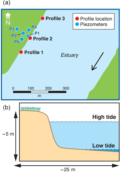
Figure 2 Location of the porewater profiles (a) and a schematic cross section of the intertidal zone (b). Also indicated is part of the piezometer network previously installed at the site, approximately aligned with the zone with the most contaminated groundwater.

The profiles were collected using a drive point system designed to collect sediment porewater at up to 1.25 m below ground surface. The drive point consisted of a 1.5 m × 24 mm outer diameter stainless steel tube to which a 10 cm drive point head was attached. The drive point head had a 5 cm screen and was connected to the surface via a 5 mm inner diameter PVC tube in order to minimise the need for purging between samples. The drive point was gently hammered at suitable depths whilst being protected from damage by a removable snugly fitting brass shoe.

2.2 Sample collection

At each location, porewater was sampled at 25 cm intervals from the channel bed surface down to 1.25 m deep (only to 1.0 m at Profile 1). This sampling interval was defined to maintain a high enough vertical resolution to capture the hyporheic zone while minimising the risk to entrain water from adjacent intervals during sample collection. At each depth, ∼65 mL was first purged using a handheld peristaltic pump. The purge water was used to collect field measurements, including for electrical conductivity, oxygen concentration, pH, temperature and redox potential using calibrated probes. A further 60 mL was then collected for major ions: 20 mL for ${\mathrm{NH}}_{\mathrm{4}}^{+}$, ${\mathrm{NO}}_{\mathrm{2}}^{-}$ and ${\mathrm{NO}}_{\mathrm{3}}^{-}$; 20 mL for radon-222; 5 mL for the stable isotopes of water; and 40 mL for the stable isotopes of nitrate. Overall, ∼210 mL of porewater was removed at each depth. Assuming a porosity ∼0.3 and that porewater was drawn to the drive point from a sphere around the screen, the radius of influence (∼6 cm) should not have overlapped between adjacent sampling depths.

Samples for major ions and nutrients were collected in 250 mL plastic containers, stored at 4 ^∘C in the field, and 0.45 µm filtered within a few hours of collection. Samples for stable isotopes of water were 0.45 µm filtered in the field and stored in 2 mL vials. Samples for the stable isotopes of nitrate were stored in 60 mL containers and kept at 4 ^∘C in the field, and they were 0.2 µm filtered and frozen within a few hours of collection. Radon-222 samples were collected following the DC method of Leaney and Herczeg (2006). Briefly, the tip of a 20 mL disposable syringe was inserted into the exit tubing from the peristaltic pump and then gently filled by pumping. An initial 6 mL sample was used to flush the syringe and remove air bubbles, followed by a 14 mL sample. The syringe was then fitted with a 0.45 µm pore-sized disposable filter and a needle. The radon sample was preserved by injecting below a mineral-oil–scintillant mixture in a pre-weighed scintillation vial.

A surface water sample was collected at the beginning (surface water −1) and at the end (surface water −2) of the sampling period. Sample collection was as for the drive point, with the exception that field parameters were measured by suspending the probes in the estuary and radon-222 was collected using the PET method (Leaney and Herczeg, 2006) to account for lower expected radon activities in surface water.

2.3 Analytical methods

Chloride and nitrogen species (${\mathrm{NH}}_{\mathrm{4}}^{+}$, ${\mathrm{NO}}_{\mathrm{3}}^{-}$ and ${\mathrm{NO}}_{\mathrm{2}}^{-}$) were determined by colorimetry at ALS Environmental in Newcastle, New South Wales. The detection limits for chloride and nitrogen species are 1 and 0.01 mg L⁻¹, respectively. Stable isotopes of water were sent for analysis to GNS New Zealand and were measured on an Isoprime mass spectrometer – for δ¹⁸O by water equilibration at 25 ^∘C using an AquaPrep device and for δ²H by reduction at 1100 ^∘C using a Eurovector Chrome HD elemental analyser. All results are reported with respect to VSMOW2, normalized to internal standards. The analytical precision for this instrument is 0.2 ‰ for δ¹⁸O and 2.0 ‰ for δ²H. The stable isotopes of nitrate samples were sent to Leeder Analytical (Melbourne) to be analysed using the bacterial denitrification method to convert ${\mathrm{NO}}_{\mathrm{3}}^{-}$ into N₂O prior to measurement by isotope ratio mass spectroscopy. Nitrate nitrogen isotope ratios are reported relative to N₂ in air and oxygen isotope ratios relative to VSMOW reference water. Internal nitrate isotopic standards were calibrated to the following standards: IAEA-${\mathrm{NO}}_{\mathrm{3}}^{-}$ (+4.7 ‰_air, 25.32 ‰_VSMOW), USGS32 (+180 ‰_air, 25.40 ‰_VSMOW), USGS34 (−1.8 ‰_air, −27.78 ‰_VSMOW) and USGS 35 (+2.7 ‰_air, 56.81 ‰_VSMOW). The precision on the nitrogen and oxygen isotopic analyses is ±0.5 ‰. Radon-222 activity was measured by liquid scintillation at CSIRO, Adelaide, with a detection limit of ∼3 and 100 mBq L⁻¹, for the PET and DC methods, respectively, with a precision of 3 %–5 %.

2.4 Interpretation

Separating the role of mixing between groundwater and surface water in the hyporheic zone from the one of attenuation during nitrogen transport in the subsurface is challenging. A simple graphical approach developed for surface water discharge to estuaries was used to differentiate the contribution between mixing and attenuation in the hyporheic zone (Ullman et al., 2003). In estuaries, river freshwater and associated nutrients mix with estuarine waters before discharging to the ocean. Tidal cycles in estuaries result in little net movement of water in or out of the estuary but generate significant mixing. This mixing is a dispersive process; i.e. solutes tend to move from high to low concentration areas even when no solvent movement occurs. Similarly, hyporheic exchange can be viewed as a dispersive process in the channel bed, with no net exchange of water but a transport of solutes from high to low concentration areas (Qian et al., 2008). In applying the concept developed for estuaries to hyporheic exchange, the discharging groundwater flowing through the hyporheic zone is considered to act as the “river”, the hyporheic zone is considered to act as the “estuary” and surface water is considered to act as the “ocean” endmember.

The dynamics of mixing in estuaries at steady state have been described by Officer (1979) and Officer and Lynch (1981):

$$\begin{array}{}\text{(5)}& F=Qc-K_{x}A{\displaystyle \frac{\mathrm{d}c}{\mathrm{d}x}},\end{array}$$

where F is the flux of a reactive solute out of the estuary, Q is river discharge, c the solute concentration in the river, K_x the longitudinal dispersion coefficient, A the cross-sectional area of the estuary and dc ∕ dx the solute concentration gradient along the estuary. The approach assumes no density stratification (i.e. the water column is perfectly mixed). At steady state the distribution of salinity (s; or any other conservative tracer) along the estuary is

$$\begin{array}{}\text{(6)}& Qs-K_{x}A{\displaystyle \frac{\mathrm{d}s}{\mathrm{d}x}}=\mathrm{0}.\end{array}$$

Incorporating the two equations, the variations in the reactive solute concentration can be expressed as a function of the variations in salinity:

$$\begin{array}{}\text{(7)}& F=Q\left(c-s{\displaystyle \frac{\mathrm{d}c}{\mathrm{d}s}}\right).\end{array}$$

The effect of attenuation and mixing on reactive solutes can be evaluated visually (Fig. 3). In the case of a solute that is entirely conservative (line A in Fig. 3), the mixing line is linear. In this case, there is no addition or removal of the solute during transport through the hyporheic zone and the solute flux out is simply Qc. However, when a solute is produced in the hyporheic zone (line B), its concentration will fall above and, when it is consumed, it will fall below the mixing line (lines C and D). The intercept of the tangent of these curves from the surface water endmember ($c_o^{*}$) is an estimate of the effective solute concentration leaving the hyporheic zone. In other words, $c_o^{*}$ is the concentration that the estuary would receive if there were no mixing in the hyporheic zone, only attenuation. The solute flux out of the hyporheic zone is $Q{c}_o^{*}$. In the case where $c_o^{*}$ is negative (line D), all the groundwater input of the solute is consumed within the hyporheic zone. The negative flux $Q{c}_o^{*}$ also means that the hyporheic zone is a sink for solutes imported from the surface water by mixing.

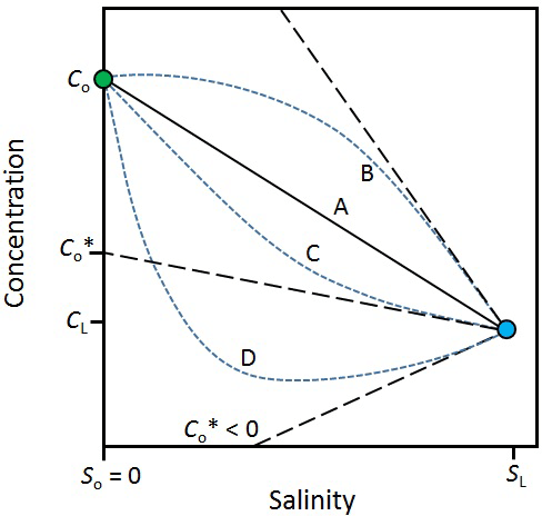
Figure 3 Variations in the concentration of a solute along a salinity gradient in an estuary. c_L, s_L – solute concentration and salinity in the sea; c_o, s_o – solute concentration and salinity in the river; line A – mixing only (no solute production or consumption in the estuary). Line B – solute production in the estuary. Lines C and D – solute consumption in the estuary; $c_o^{*}$ – effective solute concentration. The tangents off lines B, C and D (black dashed lines) are used to infer $c_o^{*}$. For line D, $c_o^{*}$ < 0, which means the estuary is also a sink for solutes imported by mixing from the sea. Modified from Officer (1979).

As in the present investigation, the hyporheic zone only covered a part of the considered depth profiles, the application of the Officer (1979) model required an adaptation. Below the hyporheic zone, it can be assumed that there is no mixing while attenuation is possible, whereas in the hyporheic zone both mixing and attenuation can occur. Thus, the profiles were interpreted in two parts: below (constant chlorinity) and within the hyporheic zone (variable chlorinity). The two key assumptions of the application of the Officer (1979) model to the hyporheic zone context are that it is assumed groundwater flow is largely vertical at the scale of the measurements and that concentration patterns are near steady state. Whilst it is customary to use salinity to evaluate mixing in estuarine environments, here chlorinity was used instead because the reactive constituents of interest can represent a significant proportion of the salinity.

3 Results

Incidental measurements of water level in the clear tubing of the drive point showed a hydraulic head ∼50 cm above river level at 1 m depth in Profile 2 and ∼0.2 m above river level at 1.25 m depth in Profile 3. This was consistent with numerous small seeps at the foot of the embankment, showing ubiquitous groundwater discharge in the intertidal zone at low tide.

3.1 Field parameters

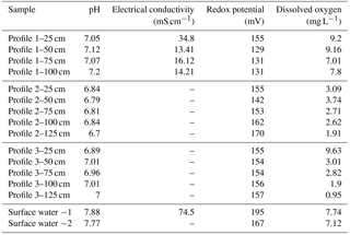
The three profiles differed markedly in their field parameters (Table 1). Relative to surface water from the estuary, porewater was less conductive, especially deeper in the profiles, and also slightly more acidic. Whilst pH was ∼7.8 in surface water, it ranged from 6.8 in Profile 2 to 7.1 in Profile 1. The most variable field parameter in the profiles was oxygen concentration. All profiles had declining O₂ with depth but over a different range. Profile 1 was well oxygenated throughout (7.8–9.2 mg L⁻¹), Profile 2 was suboxic (1.9–3.1 mg L⁻¹) and Profile 3 varied from suboxic at 1.25 m (1.0 mg L⁻¹) to well oxygenated at 25 cm (9.6 mg L⁻¹).

Table 1 Field parameters collected in porewater and surface water in the intertidal zone.

3.2 Chloride

Based on chloride, the groundwater at the base of the profiles was largely terrestrial groundwater in origin mixed with some estuarine water. The groundwater Cl⁻ concentration at nested piezometer P3 (∼140 m inland; Fig. 2) was previously found to vary between 0.028 g L⁻¹ (Unit 1) and 0.047 g L⁻¹ (Unit 2; Andrew Minard, unpublished data). By comparison, surface water was 15 g L⁻¹ at the time of sampling and porewater at the base of the profiles was 1.88, 3.29 and 8.75 g L⁻¹ for profiles 2, 1 and 3, respectively (Fig. 4a). Thus, at 100–125 cm, profiles 1 and 2 were composed of 12 %–20 % surface water while Profile 3 was 60 % surface water. In general, chloride concentrations remained constant between 75 and 125 cm but then increased upward, indicating the hyporheic mixing zone was approximately 50 cm in thickness. However, Cl⁻ concentration remained ∼8 g L⁻¹ throughout Profile 3, suggesting a thinner hyporheic zone there. Trends with depth for δ${}^{\mathrm{2}}{\mathrm{H}}_{{\mathrm{H}}_{\mathrm{2}}\mathrm{O}}$ and δ${}^{\mathrm{18}}{\mathrm{O}}_{{\mathrm{H}}_{\mathrm{2}}\mathrm{O}}$ were similar to chloride but with some subtle differences between profiles. As for Cl⁻, the isotopic composition of water indicated mixing with surface water at 25 and 50 cm (Fig. 4b–c). The Cl⁻ and δ${}^{\mathrm{2}}{\mathrm{H}}_{{\mathrm{H}}_{\mathrm{2}}\mathrm{O}}$ values for profiles 1 and 2 were similar but differed from those found in Profile 3. However, δ${}^{\mathrm{18}}{\mathrm{O}}_{{\mathrm{H}}_{\mathrm{2}}\mathrm{O}}$ was enriched by ∼2 ‰ in Profile 2 relative to Profile 1 (see additional evaluation for the isotopic composition of water below).

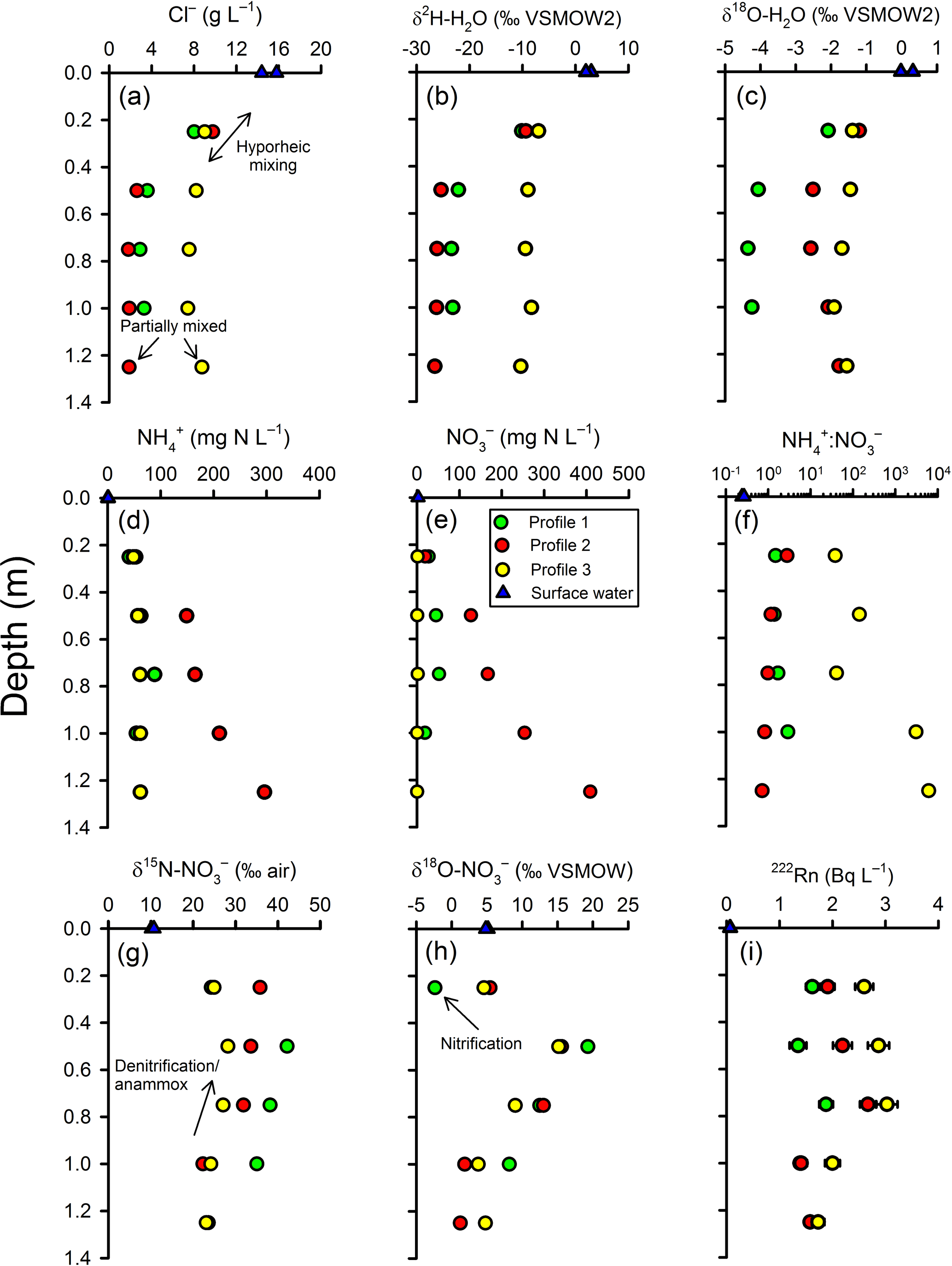
Figure 4 Intertidal zone porewater profiles for selected parameters. Based on the trends in chloride (a) and the stable isotopes of water (b–c), two scales of groundwater–surface-water mixing were apparent in the profiles. In the top 50 cm of the profiles, a gradual change in concentration between a surface water and deeper porewater endmember is consistent with hyporheic mixing. Below the hyporheic zone, chloride concentrations were relatively constant but were intermediate between terrestrial groundwater and surface water, suggesting return flow from tide-induced circulation. See text for explanations about the other parameters.

3.3 Ammonium and nitrate

There was a general trend for decreasing ${\mathrm{NH}}_{\mathrm{4}}^{+}$ and ${\mathrm{NO}}_{\mathrm{3}}^{-}$ concentrations upward in the profiles, but the extent varied materially between profiles (Fig. 4d–e). The highest concentrations were measured in Profile 2 (300–400 mg N L⁻¹ at the base) and lowest in Profile 3, especially for ${\mathrm{NO}}_{\mathrm{3}}^{-}$ (0.01–1.5 mg N L⁻¹). The decline in nitrogen concentrations was most pronounced in Profile 2, with ${\mathrm{NH}}_{\mathrm{4}}^{+}$ and ${\mathrm{NO}}_{\mathrm{3}}^{-}$ being 53 and 19 mg N L⁻¹, respectively, at 25 cm. The ${\mathrm{NH}}_{\mathrm{4}}^{+}$ to ${\mathrm{NO}}_{\mathrm{3}}^{-}$ ratio tended to increase at shallower depths in Profile 2 and decrease in Profile 3 (Fig. 4f). This means that ${\mathrm{NH}}_{\mathrm{4}}^{+}$ was lost more rapidly than ${\mathrm{NO}}_{\mathrm{3}}^{-}$ in Profile 3 while ${\mathrm{NO}}_{\mathrm{3}}^{-}$ was lost more rapidly than ${\mathrm{NH}}_{\mathrm{4}}^{+}$ in Profile 2. Nitrite was below detection limit (< 0.01 mg N L⁻¹) in porewater samples but slightly above detection limit (0.02 and 0.03 mg N L⁻¹) in the surface water samples.

3.4 Stable isotopes of ${\mathrm{NO}}_{\mathrm{3}}^{-}$

There was a consistent pattern in the isotopic composition of ${\mathrm{NO}}_{\mathrm{3}}^{-}$ as a function of depth (Fig. 4g–h). In general, δ${}^{\mathrm{15}}{\mathrm{N}}_{{\mathrm{NO}}_{\mathrm{3}}}$ and δ${}^{\mathrm{18}}{\mathrm{O}}_{{\mathrm{NO}}_{\mathrm{3}}}$ increased at first from the base of the profiles but tended to decrease once in the hyporheic zone. The increase in δ${}^{\mathrm{15}}{\mathrm{N}}_{{\mathrm{NO}}_{\mathrm{3}}}$ and δ${}^{\mathrm{18}}{\mathrm{O}}_{{\mathrm{NO}}_{\mathrm{3}}}$ deeper in the profiles would be consistent with the occurrence of a process such as denitrification (which leaves the residual ${\mathrm{NO}}_{\mathrm{3}}^{-}$ pool enriched in its heavier isotopes). However, the decreased δ¹⁵N and δ¹⁸O values once in the hyporheic zone are more difficult to evaluate. These were in part due to mixing because the isotopic composition of surface water ${\mathrm{NO}}_{\mathrm{3}}^{-}$ was less enriched than in the porewater. For example, the δ${}^{\mathrm{15}}{\mathrm{N}}_{{\mathrm{NO}}_{\mathrm{3}}}$ in surface water was 10.4 ‰ whilst it varied between 28.2 ‰ and 42.1 ‰ at 50 cm in the profiles. On the other hand, δ${}^{\mathrm{18}}{\mathrm{O}}_{{\mathrm{NO}}_{\mathrm{3}}}$ at Profile 1–25 cm was lower than in either deeper porewater or in surface water. This indicates that some nitrate with a low isotopic composition was produced in the hyporheic zone, most likely via nitrification.

3.5 Radon-222

The vertical distribution of radon-222 activity indicated a typical pattern for groundwater discharging through a hyporheic zone (Fig. 4i). In general, ²²²Rn activities ranged between 1 and 3 Bq L⁻¹ in porewater, larger than in surface water (∼0.07 Bq L⁻¹), and peaked at mid-depth. The lower activities in the hyporheic zone are likely due to mixing and the peak at mid-depth can be attributed either to groundwater “aging” along the flow path, greater radon emanation rates from sediments at the edge of the hyporheic zone, or both.

The radon emanation rate from the sediments is not known, so evaluating the apparent age of porewater is more difficult. A minimum groundwater velocity (v_low) can be estimated by assuming the largest ²²²Rn activity measured in the profiles (∼3 Bq L⁻¹) is close to equilibrium activity with sediments (A_o). Below the hyporheic zone (that is, without the need to correct for mixing), the apparent age of porewater can then be estimated from

$$\begin{array}{}\text{(8)}& A_x=A_o\left(\mathrm{1}-e^{-\mathit{\lambda }t}\right),\end{array}$$

where A_x is the radon activity at a given depth and λ the radioactive decay constant for radon. Assuming A_o ∼ 3.5 Bq L⁻¹, the time elapsed between groundwater travelling from 1.25 to 0.75 m in profiles 2 and 3 would be 4.6 and 7.2 days, respectively, resulting in a v_low of 0.11 and 0.07 m day⁻¹, respectively. However, the v_low estimates assume that the emanation rate is constant with depth, which may not be correct in the vicinity of hyporheic zones because of the potential for ²²⁶Ra (the parent to ²²²Rn) to be retained at redox interfaces (Dixon, 1990). Velocity in Profile 1 was not estimated because most samples were in the hyporheic zone, where the additional effect of mixing on radon activities would need to be considered.

An alternative estimate of velocity can be inferred from the hydraulic gradients (i) measured during sampling. Using Darcy's law, velocity would be equal to $K\cdot i/n$, with K the hydraulic conductivity of the sediments and n its effective porosity. K for a silty sand varies between 10⁻⁷ and 10⁻⁵ m s⁻¹ (Freeze and Cherry, 1979) and the vertical hydraulic gradients measured at the sites were ∼0.2–0.5 (at low tide). Assuming an effective porosity ∼ 0.3 and a hydraulic gradient ∼0.2 over the tidal cycle, velocity would be 0.006–0.6 m day⁻¹, overlapping the range found with the radon method. Thus, groundwater travelled through the 1.25 m profiles in 2 days or more.

3.6 Mixing model

In general, there was a net consumption of ${\mathrm{NH}}_{\mathrm{4}}^{+}$ and ${\mathrm{NO}}_{\mathrm{3}}^{-}$ in both the groundwater and hyporheic part of the profiles (Fig. 5). In Profile 1, ${\mathrm{NH}}_{\mathrm{4}}^{+}$ and ${\mathrm{NO}}_{\mathrm{3}}^{-}$ concentrations fell below the mixing line between groundwater and surface water, indicating consumption in the hyporheic zone. The estimated effective ${\mathrm{NH}}_{\mathrm{4}}^{+}$ and ${\mathrm{NO}}_{\mathrm{3}}^{-}$ concentrations ($c_o^{*}$) were 70 and 45 mg N L⁻¹, respectively, indicating consumption of both species. Thus, the net fraction of N consumed in the hyporheic zone (f= ($c_o^{*}-c_i$) ∕ c_i) was −0.21 and −0.13 for ${\mathrm{NH}}_{\mathrm{4}}^{+}$ and ${\mathrm{NO}}_{\mathrm{3}}^{-}$, respectively. In Profile 2, there was a large net consumption of ${\mathrm{NH}}_{\mathrm{4}}^{+}$ and ${\mathrm{NO}}_{\mathrm{3}}^{-}$ in both groundwater and in the hyporheic zone. For example, 59 % of the initial ${\mathrm{NO}}_{\mathrm{3}}^{-}$ at 1.25 m was apparently consumed once groundwater had reached the edge of the hyporheic zone, and a further 87 % of the remaining ${\mathrm{NO}}_{\mathrm{3}}^{-}$ was then consumed in the hyporheic zone itself. Overall, the attenuation of N in Profile 2 was notable, with the $c_o^{*}$ for ${\mathrm{NH}}_{\mathrm{4}}^{+}$ and ${\mathrm{NO}}_{\mathrm{3}}^{-}$ being 130 and 22 mg N L⁻¹, respectively, relative to concentrations at the base of the profile of 296 and 409 mg N L⁻¹, respectively. Thus, ∼80 % of the dissolved nitrogen was consumed in the channel bed before discharging to surface water at Profile 2.

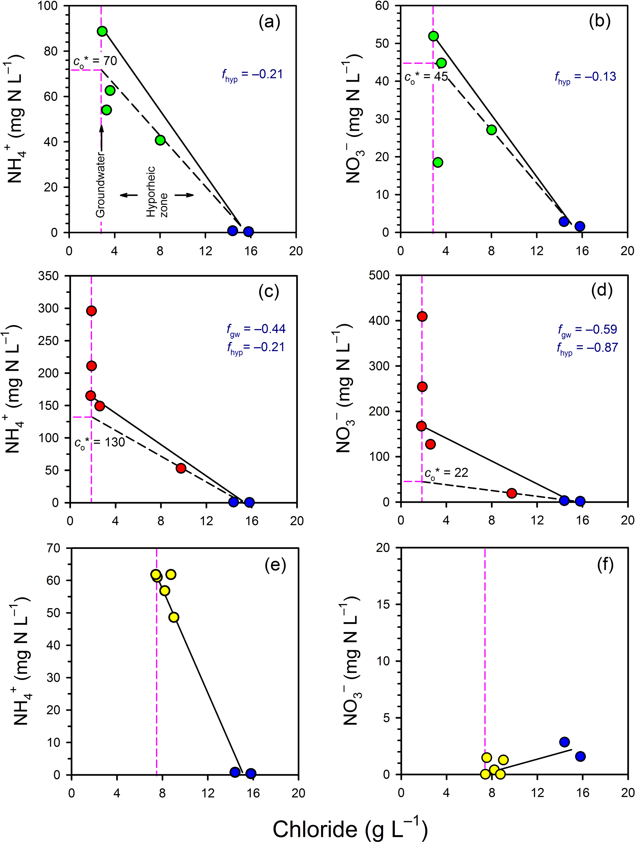
Figure 5 Evaluation of mixing and transformations for ${\mathrm{NH}}_{\mathrm{4}}^{+}$ (a, c, e) and ${\mathrm{NO}}_{\mathrm{3}}^{-}$ (b, d, f) for Profile 1 (a, b), Profile 2 (c, d) and Profile 3 (e, f). The vertical pink lines represent samples collected in the groundwater zone and those to the right of this line are within the hyporheic zone, based on chloride concentrations. The blue circles represent the surface water samples. The black solid lines represent the expected N concentrations in the hyporheic zone if only conservative mixing occurred. The black dashed lines evaluate whether N was consumed or produced in the hyporheic zone (see Fig. 3).

In Profile 3, ${\mathrm{NH}}_{\mathrm{4}}^{+}$ concentrations varied from ∼ 60 mg N L⁻¹ at the base of the profile to 48 mg N L⁻¹ closer to surface water, so some ${\mathrm{NH}}_{\mathrm{4}}^{+}$ consumption was likely. As ${\mathrm{NO}}_{\mathrm{3}}^{-}$ concentrations remained low (< 2 mg N L⁻¹) throughout the profile, if ${\mathrm{NH}}_{\mathrm{4}}^{+}$ was consumed by nitrification then denitrification probably occurred as well. The low ${\mathrm{NO}}_{\mathrm{3}}^{-}$ concentrations are consistent with the low oxygen concentrations in this profile, which would favour denitrification over nitrification. Because ${\mathrm{NO}}_{\mathrm{3}}^{-}$ concentrations in porewater were generally lower than in surface water, surface water ${\mathrm{NO}}_{\mathrm{3}}^{-}$ imported to the subsurface by hyporheic exchange was probably consumed at Profile 3 (i.e. similar to line D on Fig. 3).

3.7 Mixing models for the stable isotopes of nitrate

The variations in porewater δ${}^{\mathrm{15}}{\mathrm{N}}_{{\mathrm{NO}}_{\mathrm{3}}}$ and δ${}^{\mathrm{18}}{\mathrm{O}}_{{\mathrm{NO}}_{\mathrm{3}}}$ independent of mixing were also evaluated using the estuarine mixing model (Fig. 6). The general trends are similar between profiles. In the groundwater zone (i.e. the part of the profile below the hyporheic zone) both the δ¹⁵N and the δ¹⁸O of ${\mathrm{NO}}_{\mathrm{3}}^{-}$ became more enriched (more positive) at shallower depths, which is consistent with the occurrence of processes such as denitrification and anammox. However, in the hyporheic zone the trends were more complex. In general, isotopic enrichment continued at 50 cm but an isotopic depletion was evident at 25 cm, especially for δ${}^{\mathrm{18}}{\mathrm{O}}_{{\mathrm{NO}}_{\mathrm{3}}}$. The only exception to this pattern was δ${}^{\mathrm{15}}{\mathrm{N}}_{{\mathrm{NO}}_{\mathrm{3}}}$ in Profile 2, where the gradual enrichment persisted across the profile. Thus, attenuation processes appear to have a vertical distribution in the hyporheic zone, with evidence for greater nitrification relative to anammox and denitrification at 25 cm.

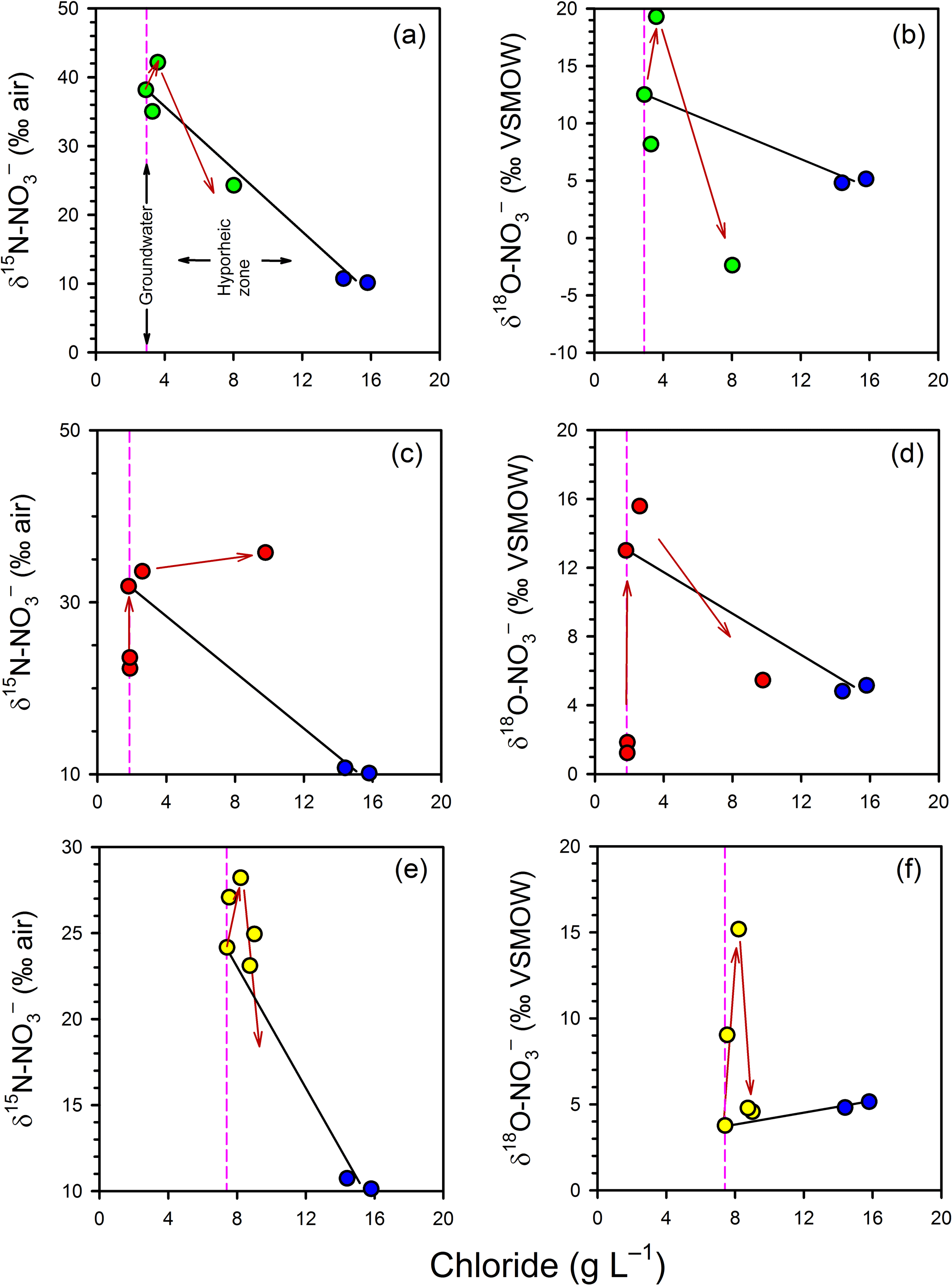
Figure 6 Evaluation of mixing and transformations for δ${}^{\mathrm{15}}{\mathrm{N}}_{{\mathrm{NO}}_{\mathrm{3}}}$ (a, c, e) and δ${}^{\mathrm{18}}{\mathrm{O}}_{{\mathrm{NO}}_{\mathrm{3}}}$ (b, d, f) for Profile 1 (a, b), Profile 2 (c, d) and Profile 3 (e, f). The vertical pink lines represent samples collected in the groundwater zone and those to the right of this line are within the hyporheic zone, based on chloride concentrations. The blue circles represent the surface water samples. The black solid lines represent expected isotopic values if only conservative mixing occurred in the hyporheic zone. The red arrows indicate the position of samples in the profiles (from bottom to top), highlighting an apparent reversal in the path of isotopic enrichment for ${\mathrm{NO}}_{\mathrm{3}}^{-}$ at the base of the hyporheic zone.

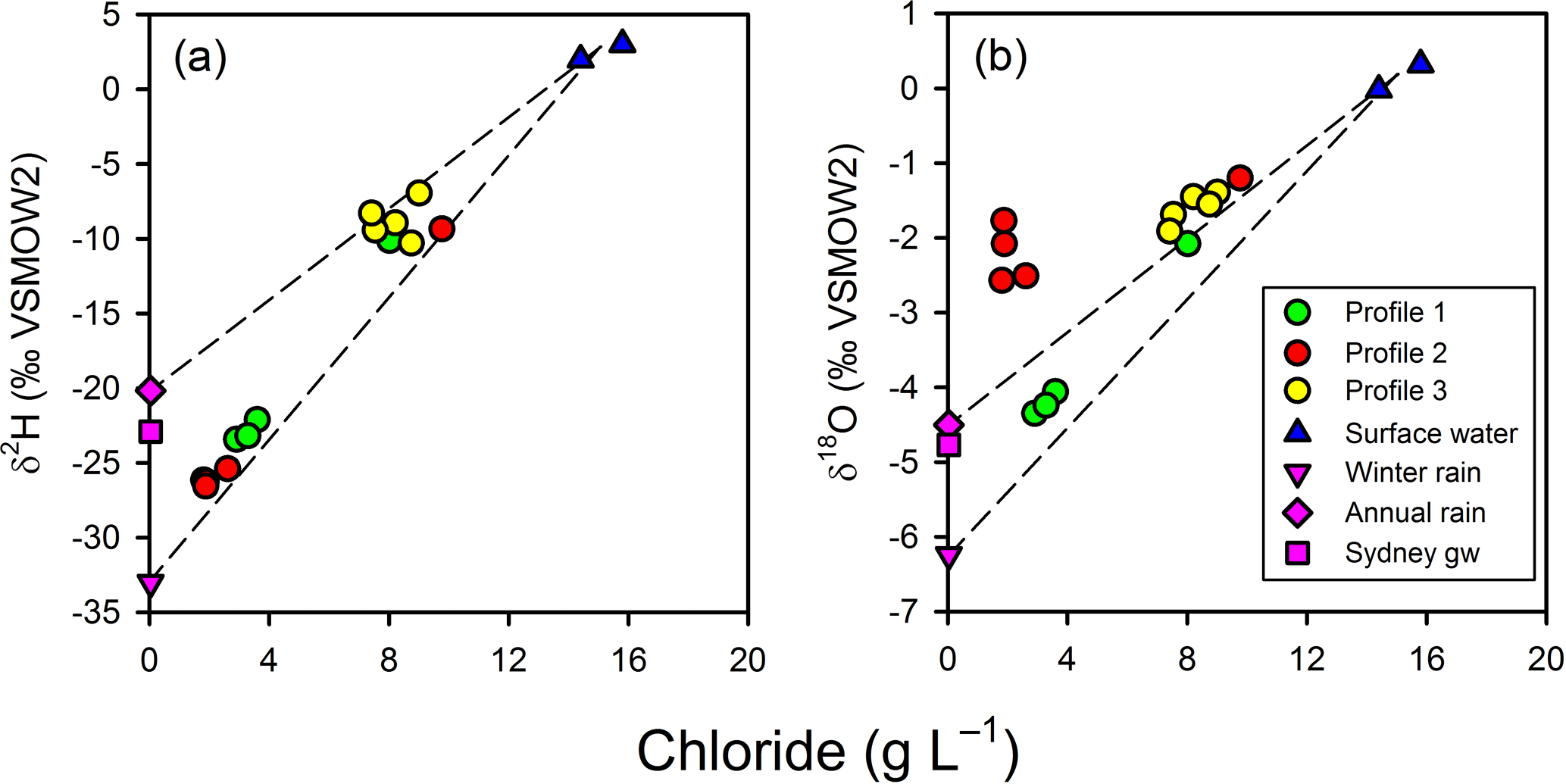
Figure 7 Chloride-based mixing lines for the isotopic composition of porewater relative to surface water and annual Sydney rainfall or winter Sydney rainfall. Sydney rainfall and groundwater were used as proxies for the isotopic composition of un-impacted groundwater at the site. Profile 2 porewater δ${}^{\mathrm{18}}{\mathrm{O}}_{{\mathrm{H}}_{\mathrm{2}}\mathrm{O}}$ values cannot be readily accounted for by a two-endmember conservative mixing model for terrestrial groundwater and surface water.

3.8 Stable isotopes of water

The observed patterns in the stable isotopes of water in the profiles were unusual. The isotopic signature of terrestrial groundwater at the site has not been measured but should be somewhere between the values associated with average annual volume-weighed precipitation (δ²H = −20.2 ‰ and δ¹⁸O = −4.50 ‰) and average annual volume-weighed winter precipitation (δ²H = −33.0 ‰ and δ¹⁸O = −6.24 ‰) for Sydney (Hughes and Crawford, 2013) or the isotopic signature for shallow groundwater in Sydney (δ²H = −22.9 ‰ and δ¹⁸O = −4.77 ‰; Hughes and Crawford, 2013). The comparison of chloride and δ${}^{\mathrm{2}}{\mathrm{H}}_{{\mathrm{H}}_{\mathrm{2}}\mathrm{O}}$ shows that the porewater samples were within expectations for mixing between two water sources (estuarine water and terrestrial groundwater), especially if the groundwater endmember was more similar to winter Sydney rainfall (Fig. 7a). However, when looking at chloride and δ${}^{\mathrm{18}}{\mathrm{O}}_{{\mathrm{H}}_{\mathrm{2}}\mathrm{O}}$ (Fig. 7b), porewater samples from profiles 2 and 3 were at least 1 ‰–4 ‰ enriched relative to conservative mixing lines and more similar to annual than winter Sydney rainfall. The discrepancy was noticeable for Profile 2 samples, especially when expressed on a δ²H-δ¹⁸O plot (Fig. 8). Water table evaporation can shift the isotopic composition of groundwater to the right of the meteoric water line (Clark and Fritz, 1997). However, evaporation would enrich both δ${}^{\mathrm{2}}{\mathrm{H}}_{{\mathrm{H}}_{\mathrm{2}}\mathrm{O}}$ and δ${}^{\mathrm{18}}{\mathrm{O}}_{{\mathrm{H}}_{\mathrm{2}}\mathrm{O}}$, whereas (relative to Sydney groundwater) Profile 2 appeared δ${}^{\mathrm{18}}{\mathrm{O}}_{{\mathrm{H}}_{\mathrm{2}}\mathrm{O}}$ enriched and possibly slightly δ${}^{\mathrm{2}}{\mathrm{H}}_{{\mathrm{H}}_{\mathrm{2}}\mathrm{O}}$ depleted. As Profile 2 is aligned with what is thought to be one of the most impacted groundwater flow lines for the site, the apparent shift in the isotopic composition of water may be related to nitrogen cycling during transport within the aquifer.

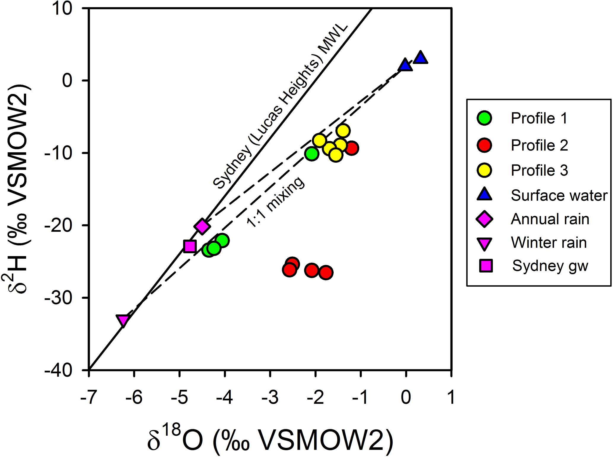
Figure 8 Isotopic composition for surface water, porewater, and Sydney groundwater and rainfall relative to the meteoric water line for Sydney (Lucas Heights; solid line). Dashed lines represent potential mixing lines between terrestrial groundwater and surface water. Note that evaporation lines for groundwater would be very similar to the mixing line in this environment. Profile 2 porewater samples do not conform to a two-endmember conservative mixing model between terrestrial groundwater and surface water.

There is also some evidence for non-conservative mixing in the isotopic composition of water at the scale of the profiles. In Profile 2, there was a gradual −1.4 ‰ shift in δ${}^{\mathrm{18}}{\mathrm{O}}_{{\mathrm{H}}_{\mathrm{2}}\mathrm{O}}$ upwards once mixing was accounted for (Fig. 9), mirroring the increase in δ${}^{\mathrm{18}}{\mathrm{O}}_{{\mathrm{NO}}_{\mathrm{3}}}$ in the same profile. This depletion was small but still above the precision for δ${}^{\mathrm{18}}{\mathrm{O}}_{{\mathrm{H}}_{\mathrm{2}}\mathrm{O}}$ measurements (< 0.2 ‰). The depletion may be an artefact of groundwater flow being in two dimensions in the intertidal zone, where different flow paths with slightly different signatures would be sampled with depth, or of temporal variations in the isotopic signature of surface water. However, in both cases variations in δ${}^{\mathrm{18}}{\mathrm{O}}_{{\mathrm{H}}_{\mathrm{2}}\mathrm{O}}$ and δ${}^{\mathrm{2}}{\mathrm{H}}_{{\mathrm{H}}_{\mathrm{2}}\mathrm{O}}$ would be expected, whereas there was no apparent shift in δ${}^{\mathrm{2}}{\mathrm{H}}_{{\mathrm{H}}_{\mathrm{2}}\mathrm{O}}$ once mixing was accounted for (Fig. 9). The variations in δ${}^{\mathrm{18}}{\mathrm{O}}_{{\mathrm{H}}_{\mathrm{2}}\mathrm{O}}$ in Profile 2 may represent an isotopic shift mediated by the significant N consumption in the channel bed at that location.

4 Discussion

Many estuaries are at risk of eutrophication because of excessive N loading from industry, agriculture or other sources (Nixon, 1995; Cosme and Hauschild, 2017). However, a mitigating feature found in many catchments is that groundwater–surface-water interactions tend to lower the N load to estuaries by fostering a biogeochemical environment where N is attenuated by denitrification or other processes (Gomez-Velez et al., 2015; Heiss et al., 2017; Kim et al., 2017). At the site, up to 80 % of the N in impacted groundwater is removed at the scale of the channel bed and N concentrations are diluted by a factor of 2 or more in the subsurface by mixing. There are also at least two scales of mixing at this site. At the larger scale, tide-induced circulation mixes surface and groundwater at the scale of tens of metres (based on chloride trends in the piezometer network; Andrew Minard, unpublished data), which is consistent with findings elsewhere (Pool et al., 2015). The degree of mixing by tide-induced circulation may be variable in space along the beach face, as suggested by the differences in chloride concentrations at the base of the porewater profiles. At the smaller scale, there was also a 50 cm hyporheic-like mixing zone in the channel bed, where tides, currents and waves would induce surface water to move in and out of the sediments. The extent of attenuation at the larger scale of mixing is not known because sampling focussed at the scale of the channel bed. Thus, the potential for N attenuation during groundwater–surface-water mixing at this site is probably larger than the 80 % of the N input estimated at the channel bed scale. Even when using a low estimate of the vertical groundwater velocity (∼0.01 m day⁻¹), this represents a very high N removal rate (> 100 mmol m⁻² day⁻¹) for permeable intertidal sediments (Schutte et al., 2015).

Figure 9 Mixing model for the isotopic composition of water for Profile 2, showing a small depletion trend upward in the profiles for δ${}^{\mathrm{18}}{\mathrm{O}}_{{\mathrm{H}}_{\mathrm{2}}\mathrm{O}}$ (a) but not δ${}^{\mathrm{2}}{\mathrm{H}}_{{\mathrm{H}}_{\mathrm{2}}\mathrm{O}}$ (b). The red arrows indicate the position of the samples in the profile, from bottom to top, highlighting that the depletion trend for δ${}^{\mathrm{18}}{\mathrm{O}}_{{\mathrm{H}}_{\mathrm{2}}\mathrm{O}}$ is continuous. When corrected for mixing, δ${}^{\mathrm{18}}{\mathrm{O}}_{{\mathrm{H}}_{\mathrm{2}}\mathrm{O}}$ would be −3.2 ‰ at the top of the profile, representing a −1.4 ‰ shift relative to the base of the profile.

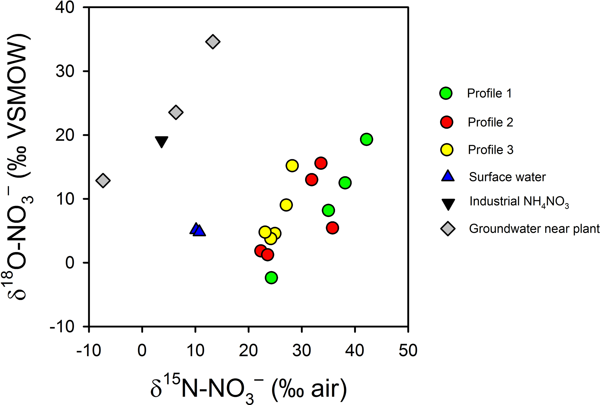
Figure 10 Variations in δ${}^{\mathrm{15}}{\mathrm{N}}_{{\mathrm{NO}}_{\mathrm{3}}}$ and δ${}^{\mathrm{18}}{\mathrm{O}}_{{\mathrm{NO}}_{\mathrm{3}}}$ in intertidal porewater, surface water, one synthetic NH₄NO₃ sample from the plant and three groundwater samples collected underneath the plant (Andrew Minard, unpublished data). The enrichment in δ${}^{\mathrm{15}}{\mathrm{N}}_{{\mathrm{NO}}_{\mathrm{3}}}$ and depletion in δ${}^{\mathrm{18}}{\mathrm{O}}_{{\mathrm{NO}}_{\mathrm{3}}}$ in porewater relative to the industrial source suggest a complete turnover of the nitrate pool during groundwater transport.

4.1 Nitrate attenuation and recycling

The trends in δ${}^{\mathrm{15}}{\mathrm{N}}_{{\mathrm{NO}}_{\mathrm{3}}}$ and δ${}^{\mathrm{18}}{\mathrm{O}}_{{\mathrm{NO}}_{\mathrm{3}}}$ suggest N is extensively recycled in the aquifer and in the channel bed. The isotopic signature for groundwater ${\mathrm{NO}}_{\mathrm{3}}^{-}$ in the source area (that is, 400 m from the river) is consistent with a synthetic NH₄NO₃ source that has been partially nitrified or denitrified (δ${}^{\mathrm{15}}{\mathrm{N}}_{{\mathrm{NO}}_{\mathrm{3}}}$ = −7 ‰ to +13 ‰ and δ${}^{\mathrm{18}}{\mathrm{O}}_{{\mathrm{NO}}_{\mathrm{3}}}$ = 13 ‰ to 35 ‰; Fig. 10). However, in the porewater profiles, ${\mathrm{NO}}_{\mathrm{3}}^{-}$ was δ¹⁵N enriched (> 20 ‰) and δ¹⁸O depleted (1 ‰–20 ‰) relative to groundwater ${\mathrm{NO}}_{\mathrm{3}}^{-}$ near the source. Thus, near the channel bed the ${\mathrm{NO}}_{\mathrm{3}}^{-}$ is largely recycled in origin, either from synthetic ${\mathrm{NH}}_{\mathrm{4}}^{+}$ that has undergone nitrification, synthetic ${\mathrm{NO}}_{\mathrm{3}}^{-}$ than was assimilated and later remineralised, or from the mineralisation of natural organic N in sediments or the aquifer (Mengis et al., 2001; Snider et al., 2010; Wong et al., 2014). Biogeochemical cycling would tend to favour ¹⁵N gradually being enriched along the flow path but for ¹⁸O to be reset with a nitrification signature once all the initial ${\mathrm{NO}}_{\mathrm{3}}^{-}$ source has been consumed.

The fractionation processes during nitrification in aquifers are not well understood but this has been evaluated in soils and in the marine environment, where δ${}^{\mathrm{18}}{\mathrm{O}}_{{\mathrm{NO}}_{\mathrm{3}}}$ is a function of the isotopic composition of the ambient dissolved O₂ and H₂O, fractionation effects during O uptake, and an isotopic equilibrium between H₂O and ${\mathrm{NO}}_{\mathrm{2}}^{-}$ (Casciotti et al., 2010). However, the isotopic equilibrium effect can probably be ignored as a first approximation because NO${}_{\mathrm{2}}^{-}$ was below detection limit in the profiles. Neglecting equilibrium effects and following Casciotti et al. (2010), the δ${}^{\mathrm{18}}{\mathrm{O}}_{{\mathrm{NO}}_{\mathrm{3}}}$ for nitrate produced via nitrification will be

$$\begin{array}{ll}{\displaystyle }& {\displaystyle }\mathit{\delta }{}^{\mathrm{18}}{\mathrm{O}}_{{\mathrm{NO}}_{\mathrm{3}}}={\displaystyle \frac{\mathrm{1}}{\mathrm{3}}}\mathit{\delta }{}^{\mathrm{18}}{\mathrm{O}}_{{\mathrm{H}}_{\mathrm{2}}\mathrm{O}}+{\displaystyle \frac{\mathrm{1}}{\mathrm{3}}}\left(\mathit{\delta }{}^{\mathrm{18}}{\mathrm{O}}_{\mathrm{2}}{-}^{\mathrm{18}}{\mathit{\epsilon }}_{\mathrm{k},{\mathrm{O}}_{\mathrm{2}}}{-}^{\mathrm{18}}{\mathit{\epsilon }}_{\mathrm{k},{\mathrm{H}}_{\mathrm{2}}\mathrm{O},\mathrm{1}}\right)\\ \text{(9)}& {\displaystyle }& {\displaystyle }+{\displaystyle \frac{\mathrm{1}}{\mathrm{3}}}\left(\mathit{\delta }{}^{\mathrm{18}}{\mathrm{O}}_{{\mathrm{H}}_{\mathrm{2}}\mathrm{O}}{-}^{\mathrm{18}}{\mathit{\epsilon }}_{\mathrm{k},{\mathrm{H}}_{\mathrm{2}}\mathrm{O},\mathrm{2}}\right),\end{array}$$

where ${}^{\mathrm{18}}{\mathit{\epsilon }}_{\mathrm{k},{\mathrm{O}}_{\mathrm{2}}}{-}^{\mathrm{18}}{\mathit{\epsilon }}_{\mathrm{k},{\mathrm{H}}_{\mathrm{2}}\mathrm{O},\mathrm{1}}$ is the combined kinetic fractionation factor during nitritation and ${}^{\mathrm{18}}{\mathit{\epsilon }}_{\mathrm{k},{\mathrm{H}}_{\mathrm{2}}\mathrm{O},\mathrm{2}}$ the kinetic fractionation factor during nitratation. Using a porewater δ${}^{\mathrm{18}}{\mathrm{O}}_{{\mathrm{H}}_{\mathrm{2}}\mathrm{O}}$ $\sim -\mathrm{1}$ ‰, ${}^{\mathrm{18}}{\mathit{\epsilon }}_{\mathrm{k},{\mathrm{O}}_{\mathrm{2}}}{-}^{\mathrm{18}}{\mathit{\epsilon }}_{\mathrm{k},{\mathrm{H}}_{\mathrm{2}}\mathrm{O},\mathrm{1}}$ ∼30 ‰, ${}^{\mathrm{18}}{\mathit{\epsilon }}_{\mathrm{k},{\mathrm{H}}_{\mathrm{2}}\mathrm{O},\mathrm{2}}$ ∼ 15 ‰ (Casciotti et al., 2010), and assuming δ¹⁸O₂ ∼23 ‰, the δ${}^{\mathrm{18}}{\mathrm{O}}_{{\mathrm{NO}}_{\mathrm{3}}}$ of ${\mathrm{NO}}_{\mathrm{3}}^{-}$ produced via nitrification in the channel bed would be approximately −8 ‰. Thus, the inference for enhanced nitrification at Profile 1–25 cm based on the low δ${}^{\mathrm{18}}{\mathrm{O}}_{{\mathrm{NO}}_{\mathrm{3}}}$ (−2.4 ‰) is reasonable.

Below the hyporheic zone, there is a tendency for porewater δ${}^{\mathrm{15}}{\mathrm{N}}_{{\mathrm{NO}}_{\mathrm{3}}}$ and δ${}^{\mathrm{18}}{\mathrm{O}}_{{\mathrm{NO}}_{\mathrm{3}}}$ to become more enriched during transport to the surface. Such a dual enrichment in the isotopic composition of ${\mathrm{NO}}_{\mathrm{3}}^{-}$ is commonly found in aquifers undergoing denitrification. The fractionation factors previously found for denitrification (${}^{\mathrm{15}}{\mathit{\epsilon }}_{{\mathrm{NO}}_{\mathrm{3}}\to {\mathrm{N}}_{\mathrm{2}}}=$ 9 ‰–20 ‰ and ${}^{\mathrm{18}}{\mathit{\epsilon }}_{{\mathrm{NO}}_{\mathrm{3}}\to {\mathrm{N}}_{\mathrm{2}}}=$ 4 ‰–16 ‰) indicate δ${}^{\mathrm{15}}{\mathrm{N}}_{{\mathrm{NO}}_{\mathrm{3}}}$ should increase faster than δ${}^{\mathrm{18}}{\mathrm{O}}_{{\mathrm{NO}}_{\mathrm{3}}}$ in the profiles. However, for porewater below the hyporheic zone the reverse pattern occurred, with δ${}^{\mathrm{18}}{\mathrm{O}}_{{\mathrm{NO}}_{\mathrm{3}}}$ increasing ∼1.5 times faster than δ${}^{\mathrm{15}}{\mathrm{N}}_{{\mathrm{NO}}_{\mathrm{3}}}$. As both ${\mathrm{NH}}_{\mathrm{4}}^{+}$ and ${\mathrm{NO}}_{\mathrm{3}}^{-}$ concentrations were elevated (> 300 mg N L⁻¹) and both were apparently consumed during transport in the profiles, anammox probably occurred. Denitrification and anammox can co-occur because a source of ${\mathrm{NO}}_{\mathrm{2}}^{-}$ (an intermediate product in denitrification) must be present to fuel anammox (Teixeira et al., 2016). In the marine pelagic zone, anammox yields a residual ${\mathrm{NH}}_{\mathrm{4}}^{+}$ pool that is ¹⁵N enriched and a ${\mathrm{NO}}_{\mathrm{3}}^{-}$ product pool that is also ¹⁵N enriched because ${\mathrm{NO}}_{\mathrm{2}}^{-}$ is either converted to ${\mathrm{NO}}_{\mathrm{3}}^{-}$ or N₂ (Brunner et al., 2013). The systematics of the oxygen isotopes during anammox are unknown so the impact this process would have on δ${}^{\mathrm{18}}{\mathrm{O}}_{{\mathrm{NO}}_{\mathrm{3}}}$ is unclear. However, the faster increase in δ${}^{\mathrm{18}}{\mathrm{O}}_{{\mathrm{NO}}_{\mathrm{3}}}$ relative to δ${}^{\mathrm{15}}{\mathrm{N}}_{{\mathrm{NO}}_{\mathrm{3}}}$ in the profiles suggests anammox more strongly fractionates ¹⁸O relative to denitrification. Overall, the shifts in the isotopic composition of ${\mathrm{NO}}_{\mathrm{3}}^{-}$ during transit through the channel bed were consistent with N attenuation via a combination of denitrification, anammox and nitrification.

These findings appear at odds with other studies from tropical and subtropical estuaries suggesting DNRA is a dominant ${\mathrm{NO}}_{\mathrm{3}}^{-}$ removal processes in sediments (Dunn et al., 2012, 2013; Dong et al., 2011). Some level of DNRA is likely in this environment and would similarly contribute to the observed trends in the ${\mathrm{NO}}_{\mathrm{3}}^{-}$ isotopes. However, DNRA cannot account for the similar variations in ${\mathrm{NH}}_{\mathrm{4}}^{+}$ and ${\mathrm{NO}}_{\mathrm{3}}^{-}$ concentrations in the profiles. If DNRA was dominant, ${\mathrm{NO}}_{\mathrm{3}}^{-}$ would decline whilst ${\mathrm{NH}}_{\mathrm{4}}^{+}$ would increase. This discrepancy with other subtropical estuaries can be attributed to the nature of the groundwater N contamination source, where a large 1:1 molar input of ${\mathrm{NH}}_{\mathrm{4}}^{+}$ and ${\mathrm{NO}}_{\mathrm{3}}^{-}$ would favour anammox over DNRA.

4.2 Stable isotopes of water

The high input and turnover of synthetic ${\mathrm{NO}}_{\mathrm{3}}^{-}$ in the aquifer during transit towards the channel bed apparently shifted the isotopic composition of groundwater. The systematics for isotopic fractionation are poorly described for groundwater (Green et al., 2010) and unknown for oxygen for anammox (Casciotti, 2016; Brunner et al., 2013). However, some preliminary assessments can be made to determine whether the magnitude of the N transformations in the aquifer can realistically shift the isotopic signature for groundwater.

The past ${\mathrm{NH}}_{\mathrm{4}}^{+}$ and ${\mathrm{NO}}_{\mathrm{3}}^{-}$ inputs from the source to the terrestrial groundwater and subsequent transit time before discharge to the river are not known. As a consequence, the initial N concentration for groundwater discharging to the river at the time of sampling is not known. However, N concentrations in excess of 5000 mg N L⁻¹ (> 0.35 mol L⁻¹) have been recently measured in groundwater near the source area (Andrew Minard, unpublished data), indicating initial N concentrations in groundwater currently discharging to the river could also have been high. Assuming an initial concentration of 5000 mg N-${\mathrm{NO}}_{\mathrm{3}}^{-}$ L⁻¹ (∼1 mol O-NO₃ L⁻¹) with a δ${}^{\mathrm{18}}{\mathrm{O}}_{{\mathrm{NO}}_{\mathrm{3}}}$ = 20 ‰, and an initial groundwater δ${}^{\mathrm{18}}{\mathrm{O}}_{{\mathrm{H}}_{\mathrm{2}}\mathrm{O}}$ = −4.8 ‰ (or δ¹⁸O_i) for discharging groundwater at the time of the study, the shift in isotopic signature if all the O-${\mathrm{NO}}_{\mathrm{3}}^{-}$ was converted in O-H₂O during transit would be

$$\begin{array}{}\text{(10)}& m_{\mathrm{tot}}\mathit{\delta }{{}^{\mathrm{18}}\mathrm{O}}_{\mathrm{tot}}=m_i\mathit{\delta }{{}^{\mathrm{18}}\mathrm{O}}_i+m_{\mathrm{O}-{\mathrm{NO}}_{\mathrm{3}}}\mathit{\delta }{}^{\mathrm{18}}{\mathrm{O}}_{{\mathrm{NO}}_{\mathrm{3}}},\end{array}$$

where m_tot is the moles of water in the final unit volume, m_i is the molarity of water (∼55.6 mol L⁻¹) and $m_{\mathrm{O}-{\mathrm{NO}}_{\mathrm{3}}}$ the moles of water produced by the consumption of ${\mathrm{NO}}_{\mathrm{3}}^{-}$ in the initial litre of reactants. Rearranging and solving for δ¹⁸O_tot yields (for $m_{\mathrm{O}-{\mathrm{NO}}_{\mathrm{3}}}$ = 1 mol L⁻¹) an isotopic signature of −4.4 ‰ or a 0.4 ‰ enrichment relative to the initial groundwater (noting that the initial volume of water would also have had to increase by 1.8 % to account for the new H₂O produced). This is smaller than the apparent level of δ${}^{\mathrm{18}}{\mathrm{O}}_{{\mathrm{H}}_{\mathrm{2}}\mathrm{O}}$ enrichment seen in profiles 2 and 3 (1 ‰–4 ‰). In part, this can be explained by a potentially larger ${\mathrm{NO}}_{\mathrm{3}}^{-}$ concentration at the source. For example, for $m_{\mathrm{O}-{\mathrm{NO}}_{\mathrm{3}}}=$ 4 mol L⁻¹ (∼20 g N-${\mathrm{NO}}_{\mathrm{3}}^{-}$ L⁻¹), the expected enrichment would be 1.7 ‰ .

Another possibility is that N cycling also promotes a broader isotopic turnover for the water pool. Many biogeochemical processes consume water, produce water or both. For example, the stoichiometry of denitrification by organic matter (Eq. 2) can also be expressed in terms of the gross amounts of water consumed and produced:

$$\begin{array}{ll}{\displaystyle }& {\displaystyle }{\left({\mathrm{CH}}_{\mathrm{2}}\mathrm{O}\right)}_{\mathrm{106}}{\left({\mathrm{NH}}_{\mathrm{3}}\right)}_{\mathrm{16}}\left({\mathrm{H}}_{\mathrm{3}}{\mathrm{PO}}_{\mathrm{4}}\right)+\mathrm{94.4}{\mathrm{NO}}_{\mathrm{3}}^{-}+\mathrm{92.4}{\mathrm{H}}^{+}\\ {\displaystyle }& {\displaystyle }+\mathrm{138}{\mathrm{H}}_{\mathrm{2}}\mathrm{O}\to \mathrm{106}{\mathrm{CO}}_{\mathrm{2}}+\mathrm{55.2}{\mathrm{N}}_{\mathrm{2}}+{\mathrm{HPO}}_{\mathrm{4}}^{-\mathrm{2}}\\ \text{(11)}& {\displaystyle }& {\displaystyle }+\mathrm{315.2}{\mathrm{H}}_{\mathrm{2}}\mathrm{O}.\end{array}$$

In this case, every mole of O-${\mathrm{NO}}_{\mathrm{3}}^{-}$ consumed also consumes ∼0.5 mol of water as well as producing ∼1.1 mol of new H₂O. Water consumption during N cycling typically enriches the remaining water pool (Buchwald et al., 2012; Casciotti et al., 2010). For demonstration purposes, Eq. (9) can be expanded by assuming that for each mole of O-${\mathrm{NO}}_{\mathrm{3}}^{-}$ consumed, 0.5 mol of H₂O is also consumed (m_c), with a ${}^{\mathrm{18}}{\mathit{\epsilon }}_{{\mathrm{H}}_{\mathrm{2}}\mathrm{O}\to \mathrm{Product}}=$ 20 ‰:

$$\begin{array}{ll}{\displaystyle }& {\displaystyle }{m}_{\mathrm{tot}}\mathit{\delta }{{}^{\mathrm{18}}\mathrm{O}}_{\mathrm{tot}}=m_i\mathit{\delta }{{}^{\mathrm{18}}\mathrm{O}}_i+m_{\mathrm{O}-{\mathrm{NO}}_{\mathrm{3}}}\mathit{\delta }{}^{\mathrm{18}}{\mathrm{O}}_{{\mathrm{NO}}_{\mathrm{3}}}\\ \text{(12)}& {\displaystyle }& {\displaystyle }-m_c(\mathit{\delta }{{}^{\mathrm{18}}\mathrm{O}}_i-{}^{\mathrm{18}}{\mathit{\epsilon }}_{{\mathrm{H}}_{\mathrm{2}}\mathrm{O}\to \mathrm{Product}}).\end{array}$$

Including isotopic fractionation during water consumption, for 1 O-${\mathrm{NO}}_{\mathrm{3}}^{-}$ mol L⁻¹ consumed the shift in groundwater δ${}^{\mathrm{18}}{\mathrm{O}}_{{\mathrm{H}}_{\mathrm{2}}\mathrm{O}}$ then doubles to −3.96 ‰ (or a ∼0.8 ‰ enrichment). As there are several potential kinetic and equilibrium fractionation effects involving water during N cycling (Brunner et al., 2013; Casciotti et al., 2010), the magnitude of the δ${}^{\mathrm{18}}{\mathrm{O}}_{{\mathrm{H}}_{\mathrm{2}}\mathrm{O}}$ enrichment associated with N attenuation at the site could be greater. In particular, whilst isotopic exchange equilibrium between ${\mathrm{NO}}_{\mathrm{3}}^{-}$ and H₂O is extremely slow at neutral pHs (Kaneko and Poulson, 2013), it can be significant when a pool of ${\mathrm{NO}}_{\mathrm{2}}^{-}$ is present (Casciotti et al., 2010). Despite many uncertainties, the apparent shift in δ${}^{\mathrm{18}}{\mathrm{O}}_{{\mathrm{H}}_{\mathrm{2}}\mathrm{O}}$ in profiles 2 and 3 relative to expectations for rainfall-derived groundwater can be reasonably accounted for by the elevated synthetic ${\mathrm{NO}}_{\mathrm{3}}^{-}$ input and its recycling during transport in the aquifer.

If the input of O-${\mathrm{NO}}_{\mathrm{3}}^{-}$ to the aquifer was sufficient to shift the δ${}^{\mathrm{18}}{\mathrm{O}}_{{\mathrm{H}}_{\mathrm{2}}\mathrm{O}}$, the similar input of ${\mathrm{NH}}_{\mathrm{4}}^{+}$ could also have shifted the δ${}^{\mathrm{2}}{\mathrm{H}}_{{\mathrm{H}}_{\mathrm{2}}\mathrm{O}}$ as ${\mathrm{NH}}_{\mathrm{4}}^{+}$ was nitrified or converted into N₂ by anammox during transport in the aquifer. Synthetic ${\mathrm{NH}}_{\mathrm{4}}^{+}$ sources appear to have a large range δ${}^{\mathrm{2}}{\mathrm{H}}_{{\mathrm{NH}}_{\mathrm{4}}}$ (∼60 ‰; Benson et al., 2009), so the potential exists for a large difference in δ²H content between synthetic ${\mathrm{NH}}_{\mathrm{4}}^{+}$ and ambient groundwater at the site. However, the porewater δ${}^{\mathrm{2}}{\mathrm{H}}_{{\mathrm{H}}_{\mathrm{2}}\mathrm{O}}$ is within expectations for mixing between winter Sydney rainfall and seawater (but not for Sydney groundwater and seawater). Thus, there is either no effect on δ${}^{\mathrm{2}}{\mathrm{H}}_{{\mathrm{H}}_{\mathrm{2}}\mathrm{O}}$ from a large ${\mathrm{NH}}_{\mathrm{4}}^{+}$ input or the shift was relatively small at the site. A search of the literature failed to yield any information on δ${}^{\mathrm{2}}{\mathrm{H}}_{{\mathrm{NH}}_{\mathrm{4}}}$ in the environment, so further evaluation of how a high ${\mathrm{NH}}_{\mathrm{4}}^{+}$ input could have impacted on porewater δ${}^{\mathrm{2}}{\mathrm{H}}_{{\mathrm{H}}_{\mathrm{2}}\mathrm{O}}$ is not, at present, possible.

5 Conclusion

This study demonstrated a strong potential for N attenuation at the groundwater–surface-water interface for contaminated groundwater discharging to a subtropical estuary. This finding is consistent with the literature, where this interface is considered an active environment for dilution of incoming groundwater solutes (Sawyer et al., 2013; Li et al., 1999) and for biogeochemical processes, in particular for the nitrogen cycle (Jones and Mulholland, 2000; Ullman et al., 2003; Gomez-Velez et al., 2015). However, in an estuarine setting, different scales of groundwater–surface-water mixing are present and may synergistically contribute to N attenuation. Much of the N attenuation at the site was probably via anammox, perhaps owing to the unusual composition of the contaminated groundwater (with near molar equivalents of ${\mathrm{NH}}_{\mathrm{4}}^{+}$ and ${\mathrm{NO}}_{\mathrm{3}}^{-}$ at the source). Once the systematics of oxygen isotope exchange during the N cycle in aquifers are better understood, the shifts in the isotopic composition of groundwater along a flow path could become a useful tool to evaluate dissolved nitrogen attenuation in both natural and contaminated environments.