the Creative Commons Attribution 4.0 License.
the Creative Commons Attribution 4.0 License.
 | 19 Jul 2018
Contributions of catchment and in-stream processes to suspended sediment transport in a dominantly groundwater-fed catchment
Yan Liu
Christiane Zarfl
Nandita B. Basu
Marc Schwientek
Olaf A. Cirpka
Suspended sediments impact stream water quality by increasing the turbidity and acting as a vector for strongly sorbing pollutants. Understanding their sources is of great importance to developing appropriate river management strategies. In this study, we present an integrated sediment transport model composed of a catchment-scale hydrological model to predict river discharge, a river-hydraulics model to obtain shear stresses in the channel, a sediment-generating model, and a river sediment-transport model. We use this framework to investigate the sediment contributions from catchment and in-stream processes in the Ammer catchment close to Tübingen in southwestern Germany. The model is calibrated to stream flow and suspended-sediment concentrations. We use the monthly mean suspended-sediment load to analyze seasonal variations of different processes. The contributions of catchment and in-stream processes to the total loads are demonstrated by model simulations under different flow conditions. The evaluation of shear stresses by the river-hydraulics model allows the identification of hotspots and hot moments of bed erosion for the main stem of the Ammer River. The results suggest that the contributions of suspended-sediment loads from urban areas and in-stream processes are higher in the summer months, while deposition has small variations with a slight increase in summer months. The sediment input from agricultural land and urban areas as well as bed and bank erosion increase with an increase in flow rates. Bed and bank erosion are negligible when flow is smaller than the corresponding thresholds of 1.5 and 2.5 times the mean discharge, respectively. The bed-erosion rate is higher during the summer months and varies along the main stem. Over the simulated time period, net sediment trapping is observed in the Ammer River. The present work is the basis to study particle-facilitated transport of pollutants in the system, helping to understand the fate and transport of sediments and sediment-bound pollutants.
- Article
(6150 KB) - Full-text XML
-
Supplement
(12082 KB) - BibTeX
- EndNote


Suspended sediments are comprised of fine particulate matter (Bilotta and Brazier, 2008), which is an important component of the aquatic environment (Grabowski et al., 2011). Sediment transport plays significant roles in geomorphology, e.g., floodplain formation (Kaase and Kupfer, 2016), and transport of nutrients, such as particulate phosphorus and nitrogen (Haygarth et al., 2006; Slaets et al., 2014; Scanlon et al., 2004). Fine sediments are important for creating habitats for aquatic organisms (Amalfitano et al., 2017; Zhang et al., 2016). Conversely, high suspended-sediment concentrations can have negative impacts on water quality, especially, by facilitating transport of sediment-associated contaminants, such as heavy metals (Mukherjee, 2014; Peraza-Castro et al., 2016; Quinton and Catt, 2007) and hydrophobic organic pollutants such as polycyclic aromatic hydrocarbons (PAHs) (Rügner et al., 2014; Schwientek et al., 2013b; Dong et al., 2015, 2016), polychlorinated biphenyls (PCBs), and other persistent organic pollutants (Meyer and Wania, 2008; Quesada et al., 2014). Without understanding the transport of particulate matter, stream transport of strongly sorbing pollutants cannot be understood.
An efficient approach to estimate suspended-sediment loads is by rating curves, relating concentrations of suspended sediments to discharge. By this empirical approach, however, we cannot gain any information on the sources of suspended sediments, which is important for the assessment of particle-bound pollutants. Therefore, a model considering the various processes leading to the transport of suspended sediments in streams is needed. Numerous sediment-transport models have been developed during the past decades, including empirical and physically based models. Commonly used empirical models include the Universal Soil Loss Equation (USLE) (Wischmeier and Smith, 1978) and the Sediment Delivery Distributed (SEDD) model (Ferro and Porto, 2000). The USLE was designed to estimate soil loss on the plot scale. It is incapable to deal with heterogeneities along the transport pathways of soil particles and thus cannot be applied to entire subcatchments. The SEDD model considers morphological effects at annual and event scales. The two models cannot distinguish different in-stream processes. Among the models simulating physical processes, the Water Erosion Prediction Project (WEPP) (Flanagan and Nearing, 1995), the EUROpean Soil Erosion Model (EUROSEM) (Morgan et al., 1998), the Soil and Water Assessment Tool (SWAT) (Neitsch et al., 2011), the Storm Water Management Model (SWMM) (Rossman and Huber, 2016), the Hydrological Simulation Program Fortran (HSPF) model (Bicknell et al., 2001), and the Hydrologic Engineering Center's River Analysis System (HEC–RAS) (Brunner, 2016) are widely used. WEPP and EUROSEM are applied to simulate soil erosion from hillslopes on the timescale of single storm events. The two models do not have the capability of estimating urban particles. SWAT uses a modified USLE method to calculate soil erosion from catchments. SWMM aims at simulating runoff quantity and quality from primarily urban areas, including particle accumulation and wash-off in urban areas. HSPF considers pervious and impervious land surfaces. All of these models estimate sediment productions from the catchment and model the transport in the river channel with simplified descriptions of in-stream processes by simplifying the shape of cross sections. Various sediment-transport models for river channels exist that rely on detailed river hydraulics, particularly the bottom shear stress, which controls the onset of erosion and the transport capacity of a stream for a given grain diameter (Zhang and Yu, 2017; Siddiqui and Robert, 2010). HEC–RAS solves the full one-dimensional Saint Venant equation for any type of cross section, including cases with changes in the flow regime, which is beneficial to obtaining detailed information on river hydraulics.
In this study, we present a numerical modeling framework to understand the combined contributions from catchment and in-stream processes to suspended-sediment transport. The main objectives of this study were (i) to develop an integrated sediment-transport model taking sediment-generating processes (e.g., particle accumulation and particle wash-off), and river sediment-transport processes (e.g., bed erosion and bank erosion) into consideration, (ii) to understand annual load and seasonal variations of suspended sediments from different processes, (iii) to investigate how the contributions of suspended sediments from catchment and in-stream processes change under different flow conditions, and (iv) to identify hotspots and hot moments of bed erosion. The model is applied to a specific catchment introduced in the next section, implying that model components that control the behavior of suspended sediments in this catchment are given specific attention, whereas processes of less relevance are simplified in the model formulation. All model components are made available in the Supplement to facilitate modifications that may be needed when applying the framework to catchments with different controls.
2.1 The Ammer catchment, Germany
We applied the integrated sediment transport model to the Ammer catchment, located in southwestern Germany (Fig. 1). The River Ammer is a tributary to the River Neckar within the Rhine basin. It covers approximately 130 km2 and is dominated by agricultural land use that accounts for 67 % of the total area. The hydrogeology is dominated by the middle-Triassic Upper Muschelkalk limestone formation which forms the main karstified aquifer (Selle et al., 2013). In this catchment, annual precipitation is 700–800 mm. The Ammer River, approximately 12 km long, is the main stem, with a mean discharge of ∼1 m3 s−1. It has two major tributaries, the Kochhart and Käsbach streams. Two wastewater treatment plants (WWTPs), Gäu-Ammer and Hailfingen, also contribute flow and suspended sediments to the Ammer River. During dry weather conditions, the discharge of WWTP Gäu-Ammer is 0.10–0.12 m3 s−1, and the effluent turbidity is approximately 3 NTUs (nephelometric turbidity units). The WWTP in Hailfingen is comparatively small, with flow rates of 0.012–0.015 m3 s−1, and its turbidity is in the same range as that of the WWTP Gäu-Ammer.
With the exception of a small stripe at the northeastern boundary of the study domain, highlighted by the forest land use in Fig. 1, the topography of the catchment is only slightly hilly (with mean slope of 4.2∘), which agrees with the bed rock being a carbonate platform, partially overlain by upper Triassic mudstones and loess. Soils are dominated by luvisols on loess with mostly high probability of deep infiltration and low risk of soil erosion, according to the state geological survey of the state of Baden-Württemberg (LGRB, http://maps.lgrb-bw.de, last access: 21 June 2018).
Based on the digital elevation model (DEM) of the Ammer catchment, we delineated 14 subcatchments using the watershed delineation tool of the Better Assessment Science Integrating point & Nonpoint Sources (BASINS) model (see Fig. 1). Table 1 shows the proportions of different land-use types and the areas of each subcatchment.
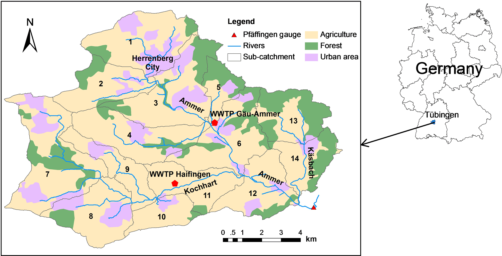
Figure 1Location of the Ammer catchment and its subcatchments, rivers, and land uses. The numbers show identifiers of 14 subcatchments that are characterized in more detail in Table 1. Two red regular pentagons represent two WWTPs in the study domain. The red triangular indicates the gauge at the catchment outlet.
Table 1Properties of the Ammer subcatchments.
∗ The agricultural land in the Ammer catchment is dominated by nonirrigated arable land (80.2 % of the total agricultural areas), the crop of which is mainly cereals with annual rotation, and complex cultivation land (e.g., vegetables, 17.5 %). The rest (2.3 %) is principally agricultural area with natural vegetation. Therefore, we summarize the three types of arable land and use the same parameterization to estimate soil erosion.
2.2 Data sources
Hourly precipitation and air-temperature data are the driving forces of the hydrological model. We use hourly precipitation data of the weather station Herrenberg, operated by the German weather service DWD (CDC, 2017), whereas air temperatures are taken from the weather station Bondorf of the agrometeorological service Baden-Württemberg (BwAm, 2016). The generation and transport of sediments behave differently for different land uses and topography. We use the digital elevation model with 10 m resolution and land-use map of the state topographic service of Baden-Württemberg and Federal Agency for Cartography and Geodesy (BKG, 2009; LGRB, 2011; UBA, 2009). The river-hydraulics model requires bathymetric profiles of the River Ammer and its main tributaries. We use 230 profiles at 100 m spacing, obtained from the environmental protection agency of Baden-Württemberg (LUBW, 2010).
Only one gauging station is installed in the main channel of the Ammer River at the outlet of the studied catchment in Pfäffingen (red triangle in Fig. 1); here, hourly discharge and turbidity measurements are available, which we used for model calibration and validation. The water levels and turbidity data were measured by online probes (UIT GmbH, Dresden, Germany). The hydrograph was converted to discharge time series by rating curves, whereas the suspended sediment concentrations are derived from continuous turbidity measurements (Rügner et al., 2013). The linear relationship between suspended-sediment concentrations and turbidity with a conversion factor of 2.02 (mg L−1 NTU−1) has been reported to be robust in the Ammer River (Rügner et al., 2013, 2014).
The simulation period covers the years 2013–2016. In this time, the maximum discharge reflected an event with a 2–10-year return period according to the long-time statistics of the gauging station (LUBW, http://www.hvz.baden-wuerttemberg.de/, last access: 21 June 2018).
3.1 Model structure and assumptions
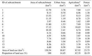
The integrated sediment-transport model consists of a catchment-scale hydrological model, a river-hydraulics model, a catchment sediment-generating model and a river sediment-transport model (Fig. 2). The catchment-scale hydrological model is used to estimate river discharge along the entire stream. The river-hydraulics model uses the discharge of the hydrological model and the river bathymetry to compute the river stage, cross-sectional area, velocity, and bottom shear stress, which are needed for the river-transport model. In this study we use HEC–RAS in quasi-steady-state mode. The catchment sediment-generating model is used for simulating particle accumulation in urban areas during dry weather periods, particle wash-off during storms, and erosion from rural areas during rain periods. The river sediment-transport model is used to simulate in-stream processes (advection, dispersion, and deposition, as well as bank and bed erosion). Wastewater treatment plants are treated as point inputs with constant discharge and sediment concentration during dry weather periods. Under low-flow conditions, when no soil erosion and urban particle wash-off occur and the suspended sediment concentrations in the streams are relatively small, we use a constant concentration to represent the sediment input under these conditions. Based on our prior knowledge of the Ammer catchment, soil erosion is very limited (the information supporting this statement will be discussed in Sect. 4.2), and thus a well-known approach and a simplified method are used to simulate particles from urban and rural areas, respectively. Mobilization of particles from different sources depends on different processes; e.g., input of urban particles depends on the build-up and wash-off processes and rural particles rely on soil erosion, whereas bed and bank erosion are substantially affected by river hydraulics. Considering these processes enables us to diagnose the importance of different sediment sources well.
Figure 2Integrated sediment transport model, consisting of a catchment-scale hydrological model, a river-hydraulic model, a sediment-generating model, and a river sediment-transport model.
3.2 Catchment-scale hydrological model
The catchment-scale hydrological model is based on the HBV model (Hydrologiska Byråns Vattenbalansavdelning) (Lindström et al., 1997). However, we have added a quick recharge component and an urban surface runoff component to explain the special behavior of discharge in the Ammer catchment (see Sect. 2.1). The main Ammer springs are fed by groundwater from the karstified middle-Triassic Muschelkalk formation. The measured hydrograph indicates a rapid increase of base flow in sporadic events. We explain this behavior with a model that contains three storages of water in the subsurface: soil moisture in the top soils, a subsurface storage in the deeper unsaturated zone, and groundwater in the karstic aquifer. In our conceptual model, we assume water storage in the deep unsaturated zone, which spills over when a threshold value is reached, causing quick groundwater recharge to occur that then leads to a rapid increase of base flow. An urban surface runoff component is used to obtain surface runoff depths in urban areas in order to simulate particle wash-off from urban land surface. Details of the hydrological model are given in Appendix A. The temporal resolution of the hydrological model is 1 h. We use the catchment-scale hydrological model to simulate discharge contributions from the 14 subcatchments shown in Fig. 1 (detailed information see Sect. 2.1).
3.3 River-hydraulics model
In order to better understand in-stream processes, we feed the discharge data of the hydrological model into the river-hydraulics model HEC–RAS (Brunner, 2016), which solves the one-dimensional Saint Venant equations. The HEC–RAS model simulates hourly quasi-steady flow using the hourly discharge of the 14 subcatchments simulated by the hydrological model as change-of-discharge input. The locations where the discharge from 14 subcatchments enters into the main channel are set to the corresponding cross sections. The upstream boundary condition was set to time series of flow and the downstream one to normal depth. We have 258 measured cross sections and we used the built-in interpolation algorithm in HEC-RAS to obtain the additional cross sections, which results in totally 385 cross sections for the entire river network. The distances between computed cross sections range from 10 to 100 m depending on the changes of river bathymetry. The model requires river profiles in cross sections along the river channel and yields the water-filled cross-sectional area, the water depth, flow velocity, and shear stress, among other factors, as model output, which are needed in the river sediment-transport model. The detailed settings of HEC–RAS can be found in the Supplement.
3.4 Sediment-generating model
The land use is classified into urban and rural areas as well as forested areas. Impervious surfaces such as roads and roofs are regarded as urban areas, while rural areas consist of pervious surfaces such as gardens, parks, and agricultural land. The sediment-generating processes are different for the two types of land use. Sediment generation in forested areas is considered to be negligible. The sediment-generating model is used to obtain hourly sediments of urban and rural particles from the 14 subcatchments.
3.4.1 Urban areas
We use the urban-area algorithm of SWMM, which performs well on particle build-up and wash-off for urban land use (Wicke et al., 2012; Gong et al., 2016), to describe sediment generation from urban areas. The corresponding processes are described below.
-
Particle accumulation. An exponential function is used to simulate particle accumulation during dry periods under the assumption that particles in the urban areas have a capacity that is governed by the accumulation process during dry periods.
in which M (g m−2) and Mmax (g m−2) represent the particle build-up at the current time and the maximum build-up (particle mass per unit area), respectively; k (s−1) is the rate constant for particle accumulation, and t (s) denotes time since the last wash-off event. The maximum build-up depends on the location because the particle production (such as traffic density, population density, and industry density) and cleaning frequency (removing urban particles) differ in different urban areas. In our model it is obtained as uniform value for the entire catchment by calibration. The particle accumulation is restarted at the beginning of every accumulation period considering remaining particles after the flush period.
-
Particle wash-off. A power function is used to simulate particle wash-off during rain periods. The particle wash-off quantity is a function of surface runoff and the initial buildup of the corresponding rain period.
in which rw (g m−2 s−1), q (m s−1), and csw (mg L−1) are the rate of wash-off, the surface runoff velocity, and the concentration of washed suspended sediment, respectively; kw (s m) and nw (–) represent a wash-off coefficient and a wash-off exponent.
3.4.2 Rural areas
In contrast to urban areas, the supply of suspended sediments from rural areas can be seen as “infinite” because they mainly originate from eroded soils. Soil erosion is assumed to linearly depend on shear stress, provided that the shear stress generated by surface runoff is larger than a critical shear stress. The sediment generation from rural areas is based on the study of Patil et al. (2012).
in which τ (N m−2) is the mean shear stress generated by the average depth of surface runoff Rsurface (m), tanθ (–) is the mean slope of the subcatchment, ρw (kg m−3) is the density of water, and g (m s−2) is the gravitational acceleration constant. The rural sediment load yh (kg m−2 s−1) is directly proportional to the difference between the mean shear stress τ and the critical rural shear stress τc (N m−2). Ch (s m−1) is a proportionality constant, csed (kg m−3) is the concentration of sediment generated in rural areas, and q (m s−1) is, like above, the surface runoff velocity. This is a simplified approach to estimate the average sediment delivery from rural areas to streams. It does not explicitly consider all processes on the hillslope scale. In particular, we do not consider the dependence of the coefficients on the crop type and time-dependent phenology of the crops. Instead, all rural areas are treated the same. We justify this strong simplification by an overall low sediment input from rural areas discussed further below. In catchments with larger sediment load from rural areas, distinctions should be made.
3.5 River sediment-transport model
We consider two types of sediment: suspended sediment in the aqueous phase (mobile component) and bed sediment (immobile component). Figure 3 shows a schematic of the river sediment-transport model, which considers advection, dispersion, deposition, bank erosion, bed erosion, and lateral input of suspended sediments. We use this model to calculate the average concentration of the mobile component and the mass of the immobile component for every computation cell (formed by two cross sections) every hour.
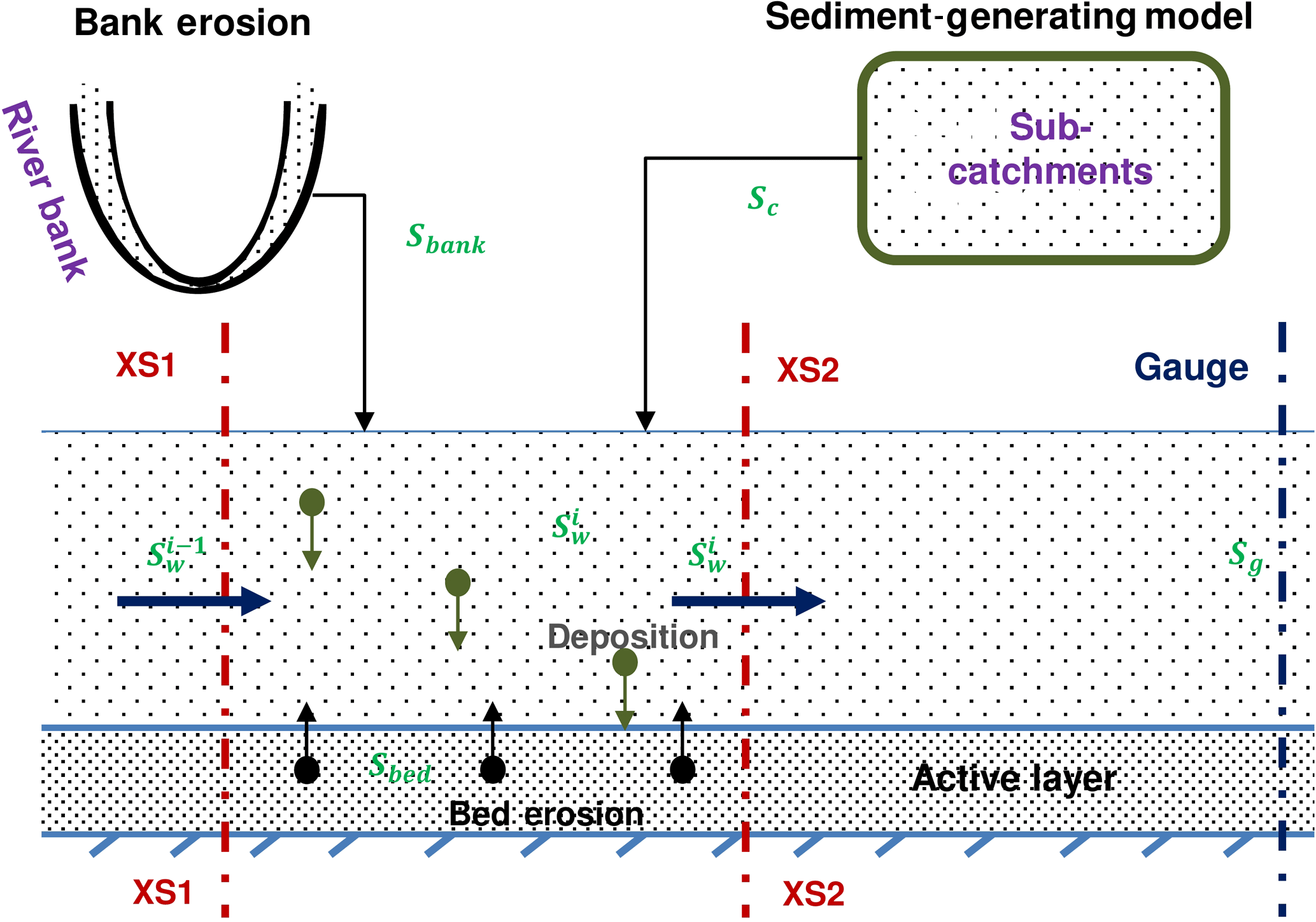
Figure 3In-stream processes of the river suspended-sediment transport model considering deposition, bed erosion, bank erosion, and input from the catchment. XS1 and XS2 are the two cross sections bounding a cell in a finite-volume scheme. Sc and Sbank are sediments from the catchment and bank erosion. Sbed indicates the bed sediment mass. stands for the concentration of suspended sediments in the ith cell. Sg is the suspended-sediment concentration at a river gauge.
-
Mobile component. We use a finite-volume discretization for suspended-sediment transport for the main channel, considering storage in the aqueous phase, advection, dispersion, bed and bank erosion, deposition, and lateral inputs (tributaries and WWTPs):
in which cw (mg L−1) is suspended-sediment concentration; V (m3) is the cell volume; Δx (m) is the cell length; Q (m3 s−1) and A (m2) are the flow rate and cross sectional area; D (m2 s−1) is the dispersion coefficient; (mg L−1) and (m3 s−1) represent the suspended-sediment concentration and flow rate of the ith lateral inflow; rd (mg L−1 s−1), rbank (g m−1 s−1), and rbed (g m−1 s−1) indicate the deposition, bed-erosion, and bank-erosion rates, respectively. For the advective term, we use upstream weighting, whereas the second derivative of concentration appearing in the dispersion term is evaluated by standard finite differences.
This model component requires the sediment concentrations in the lateral inputs (tributaries and WWTPs) as well as in the Ammer spring as boundary conditions. The lateral inputs are computed by the sediment-generating model. For the sediment input by the Ammer spring, we consider the turbidity of ∼3 NTU measured under base-flow conditions. Rügner et al. (2013) showed that the karst springs in the Ammer catchment contribute to turbidity, which is in agreement with many previous studies showing that karst systems can contribute suspended sediments (Bouchaoua et al., 2002; Meus et al., 2013). Thus, the turbidity under base-flow conditions is potentially generated by subsurface flow through the karst matrix. The karstic sediment flux was calculated by subsurface flow rates and constant suspended sediment concentrations.
-
Immobile component. For simplification, we account for one active layer only in the bed sediment per cell, and consider only the average grain size. Deposition of suspended sediments leads to a mass flux from the aqueous phase to the bed layer, whereas bed erosion causes a mass flux in the opposite direction:
in which Mbed (g m−1) is the sediment mass per unit channel length in the active layer on the river bed.
- a.
Deposition
The deposition rate rd of particles can be calculated by the following (Krone, 1962):
in which τb (N m−2) and τe (N m−2) represent the bottom shear stress of the river and the threshold shear stress of particle erosion (see below), y (m) denotes the water depth, and vs (m s−1) is the settling velocity.
- b.
Bed erosion
We consider two types of bed erosion, namely particle erosion and mass erosion, which correspond to two thresholds of the bottom shear stress. The bed erosion rate rbed can be calculated by the following (Partheniades, 1965):
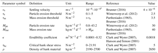
in which rbed (g m−1 s−1) is bed erosion rate; τm (N m−2) represents the mass erosion threshold, whereas Mpe (g m−1 s−1) and Mme (g m−1 s−1) are rate constants, denoting the specific rates of particle and mass erosion.
- c.
Bank erosion
In our model, the bank erosion rate rbank is calculated by the following:
in which τbank (N m−2) and τbc (N m−2) are the bank shear stress and critical shear stress for bank erosion. κ (m3 N−1 s−1) is the erodibility coefficient. ρ (kg m−3) is density of bank material. L (km) is length of the river bank.
- a.
3.6 Parameter estimation
For the estimation of parameters, we used the well-known Nash–Sutcliffe efficiency (NSE) as model performance criterion:
in which Oi and Mi are the ith observed and modeled values, is the mean of all observed values. An NSE value approaching unity indicates good agreement between model and data, whereas NSE values smaller than zero imply that the model performs worse than taking the mean of all observations. We obtained the best set of parameters by systematically scanning the parameter space.
The hydrological model was applied to 14 subcatchments. Each subcatchment has three types of land use: agricultural areas, forest, and urban areas. We used daily average discharge data of 2013–2014 and 2015–2016 for calibration and validation, respectively. We generated 1000 realizations of the 14 parameters by Latin hypercube sampling (LHS) and calculated the corresponding NSE value for each parameter set. If NSE was ≥ 0.55, the parameter set was regarded acceptable. In the same way, we used the accepted parameter sets for validation. Subsequently we calculated the 90 % confidence intervals and the NSE value for high flows (flow rate greater than the mean discharge) using the accepted parameter sets. Finally, we identified the best-fit parameter values.
For the calibration and validation of the sediment-generating and the river sediment-transport models, we performed a literature survey to identify a reference range of each parameter. We performed a manual calibration of the corresponding parameters within the given range, fitting the modeled and measured suspended sediment concentrations at the river gauge. Subsequently, we used the identified parameter set as base values in a local sensitivity analysis, the details of which are given in Table S1 of the Supplement. Within the given parameter variations, the manually calibrated parameter sets were confirmed as optimal. The parameters of the sediment-generating model and the river sediment-transport models are listed in Tables 2 and 3, respectively.
Table 2Parameters of the sediment-generating model.

a The range of k is calculated under the assumption that it takes 5–30 days to reach 90 % of the maximum buildup. b The range of Kw, 50–500, is sufficient for most urban runoff. c It is for the most of time, but depends on soil properties.
Table 3Parameters of the river sediment-transport model.
∗ This range is calculated for the suspended sediment with average diameter 1–50 µm.
4.1 Quality of model calibration and validation
The best-fit parameter set of the hydrological model resulted in NSE values of 0.63 and 0.59 for calibration and validation, respectively. Figure 4 shows the measured and simulated hydrographs for the calibration and validation periods with 90 % confidence intervals. It can be seen that the discharge was reproduced quite well, both in the general trend and the dynamics. The measured discharge data almost all fall within the 90 % confidence interval of the simulation. The NSE value for high flows (greater than the mean discharge, 1 m3 s−1) of the simulation period is 0.43, implying an acceptable fit of high flows. There are few events that cannot be reproduced by the model. These events occurred in the summer months and probably resulted from thunderstorms, which are very local and may be missed by precipitation measurements, so that the resulting flow peaks could not be predicted by the hydrological model.
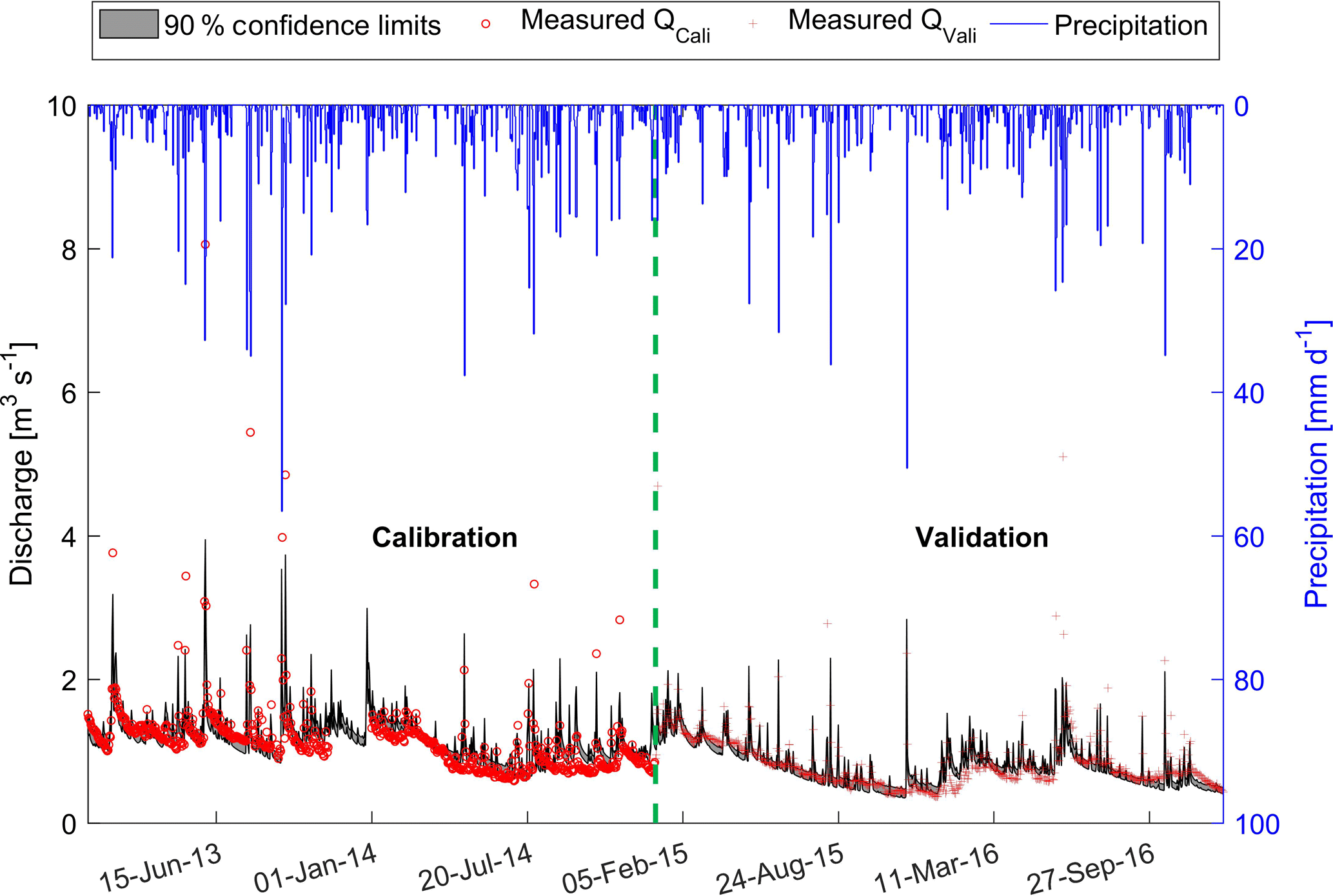
Figure 4Calibration (left, year 2013–2014) and validation (right, year 2015–2016) of hydrological model, QCali and QVali are measured discharges used for calibration and validation, respectively.
Figure 5 depicts measured suspended-sediment concentrations and the simulation results of the sediment-transport model during the calibration (year 2014) and validation (year 2016) periods. The corresponding NSE values are 0.46 and 0.32, respectively, which indicates an acceptable fit, albeit not as good as for the hydrograph. The integrated sediment transport model can capture the dynamics of the suspended sediment concentrations. In particular, the model captures the concentration peaks well. However, two events, one in the calibration and the other in the validation period, were not well fitted. These are events which were also not captured by the hydrological model, occurring in the summer months and due to thunderstorms.
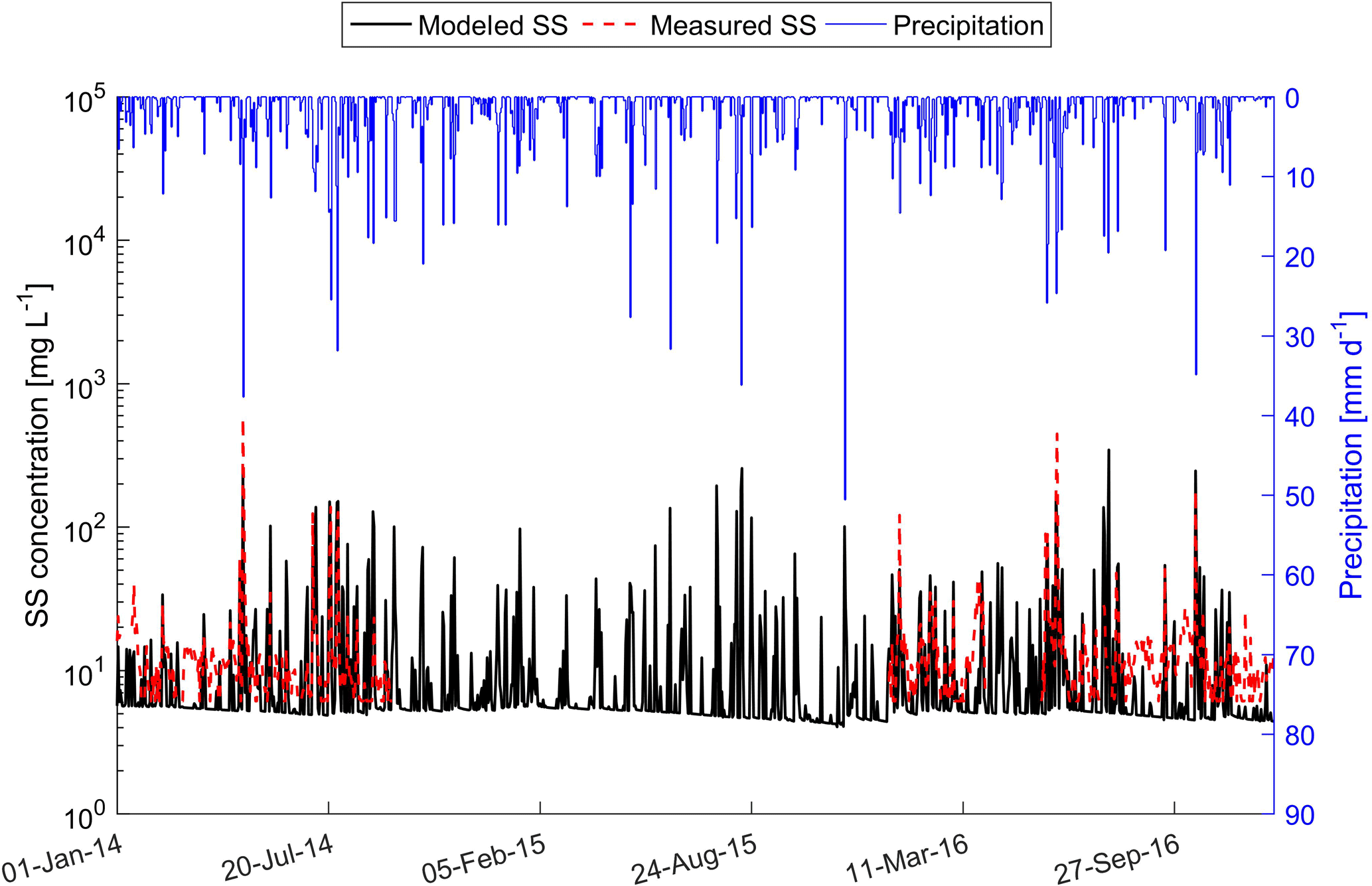
Figure 5Modeled and measured suspended sediment concentrations used for calibration (year 2014) and validation (year 2016) of the sediment transport model. A data gap exists for the year 2015.
4.2 Annual and monthly suspended sediment loads from different processes
After calibration and validation, the model results can be used to analyze the importance of different sediment sources. Figure 6 displays the modeled annual suspended-sediment loads from catchment and in-stream processes for the entire Ammer River network. The annual suspended-sediment load at the gauge ranges between 410 and 550 t yr−1. Equation (13) describes the overall mass balance of sediments in the entire catchment:
in which Loadgauge (t yr−1) indicates the suspended-sediment load at the river gauge. Loadurban (t yr−1), Loadrural (t yr−1), and Loadkarst (t yr−1) denote the suspended-sediment loads from urban areas generated by surface runoff and WWTP effluent, rural areas generated by soil erosion, and the karst system carried by subsurface flow, respectively. These three terms represent the catchment processes. Loadbde (t yr−1), Loadbke (t yr−1), Loaddep (t yr−1), and ΔS (t yr−1) are the suspended-sediment loads from bed erosion, bank erosion, deposition, and the change of sediment storage in the entire river channel, respectively. These four terms represent the in-stream processes.
In the Ammer catchment, urban particles (266–337 t yr−1) and the sediment input from the karst system (106–160 t yr−1) dominate the annual suspended sediment load, accounting for 59.1 and 24.9 %, respectively. Bed erosion, bank erosion, and rural sediment contribute much less, namely 6.2, 6.3, and 3.5 % of the total annual load, respectively. The contribution of rural runoff sediment in the Ammer catchment was very small, which may appear to be surprising at first. We have collected several independent lines of evidence that support these findings and included them in the Supplement:
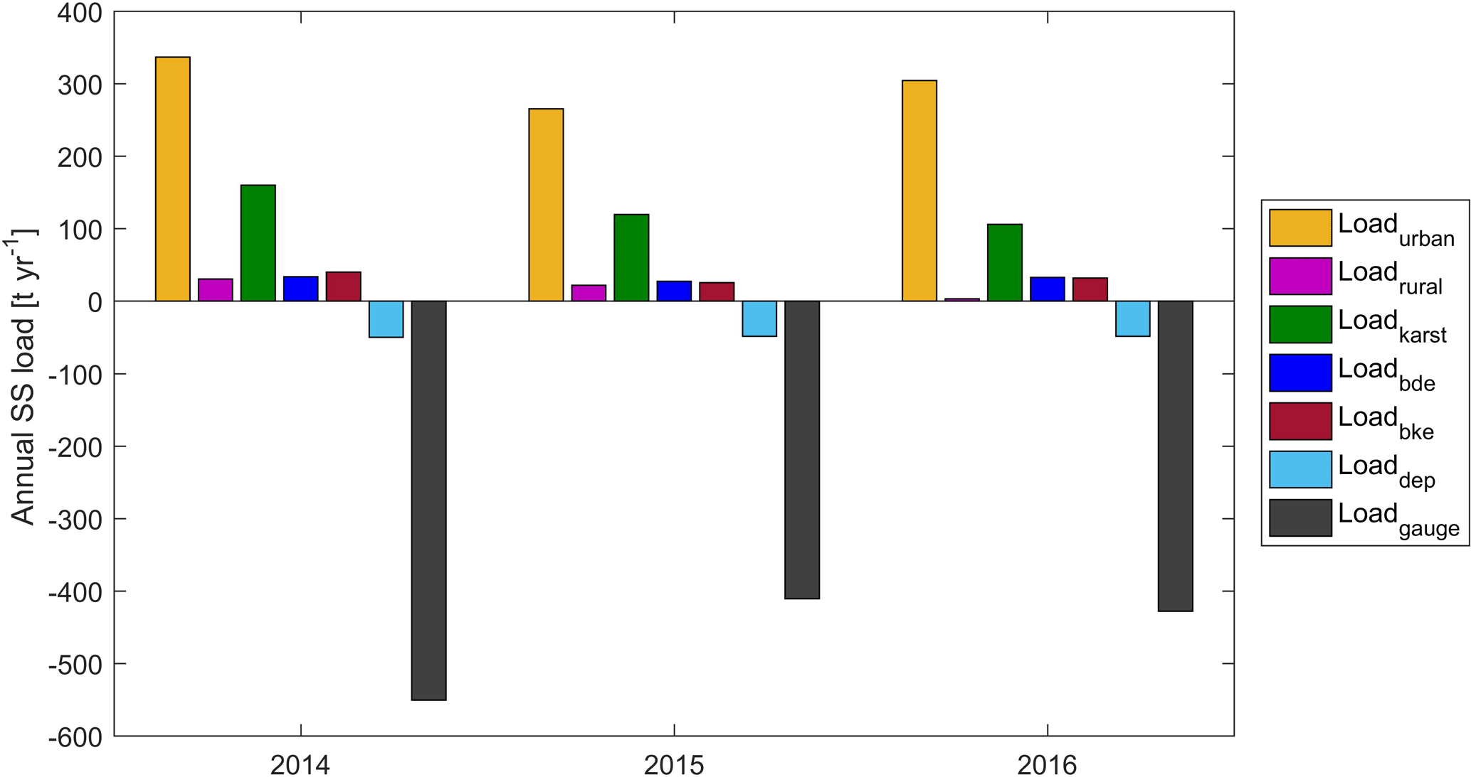
Figure 6Annual suspended sediment loads from different processes. Loadgauge is calculated by modeled discharge and suspended sediment concentrations at catchment outlet. Loadurban, Loadrural, and Loadkarst are calculated using the results of sediment-generating model. Loaddep, Loadbde, and Loadbke are the sum of deposition load, suspended sediments eroded from river bed and river bank of the entire river network for a whole year, respectively. In this figure, the positive values represent sediment input to the river channel, while negative values denote sediment output from the river channel.
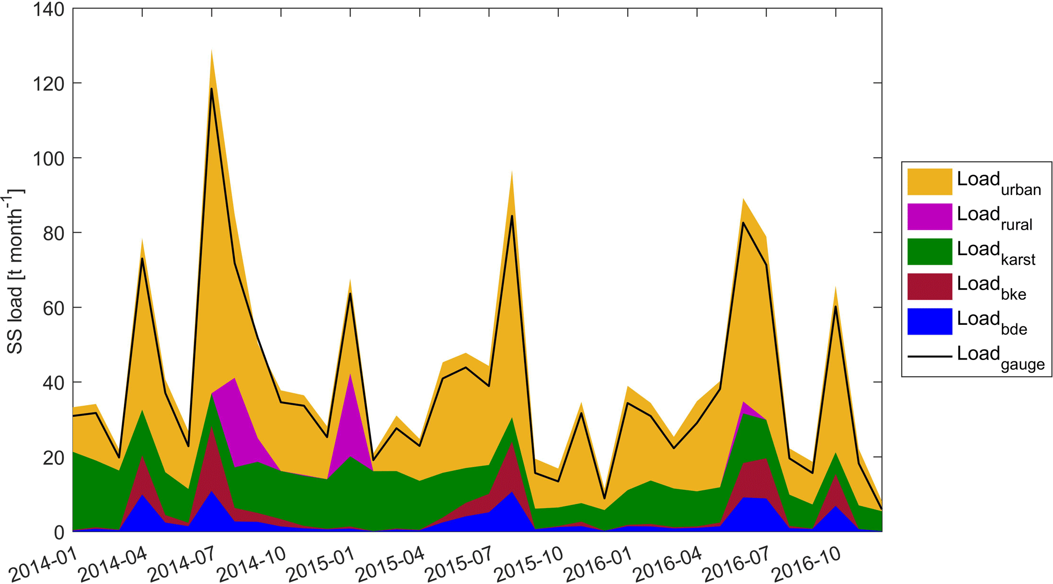
Figure 7Monthly mean suspended-sediment load from different processes, calculated using the model results of 2014–2016. Loadgauge, Loadurban, Loadrural, and Loadkarst are the monthly mean suspended-sediment load at the gauge and from urban areas, rural areas, and the karst system. Loadbke and Loadbde represent monthly mean suspended-sediment load from bank erosion and bed erosion for the entire river network, respectively. The area above the line of Loadgauge is the monthly mean deposition, Loaddep.
The suspended sediments of the Ammer River are strongly contaminated by polycyclic aromatic hydrocarbons and other persistent organic pollutants (Schwientek et al., 2013b). Table S2 and Eqs. (S1)–(S7) of the Supplement present an end-member-mixing analysis indicating a fraction of rural particles amounting to only 3 %.
The state geological survey of the state of Baden-Württemberg has developed a soil-erosion risk map shown Fig. S1, putting most of Ammer catchment into the class of lowest soil-erosion risk. This is so because the surface runoff from agricultural areas is small due to a comparably flat topography. The same agency associates most of the catchment with deep infiltration as the main discharge mechanism.
Schwientek et al. (2013a) found a lacking connection between soils and streams in the Ammer catchment. The catchment has a large water storage capacity due to the karst and the slopes of this catchment are mild. During the simulation period, the precipitation intensity was not large enough to exceed the maximum infiltration rates or to reach storage capacity of the subsurface. Compared with literature values of maximum infiltration rates (10–20 and 5–10 mm h−1 for loamy soil and clay loamy soil, respectively; http://www.fao.org/docrep/S8684E/s8684e0a.htm, last access: 21 June 2018), only a few events exceed 10 mm h−1 of the precipitation intensity during the simulation period. Thus, hardly any surface runoff occurred in the rural area, so that sediment generation and transport from rural areas to the river channel were small.
The comparably flat topography can be explained by the geological formation. The Muschelkalk limestone is a carbonate platform that is partially overlain by mudstones of the upper Triassic. Along the Ammer main stem, there is only a small stretch where the river is incised somewhat deeper into the limestone rock. The river lost its former headwater catchment in the early Pleistocene to river Nagold so that the currently existing small river has a too-wide valley given its discharge.
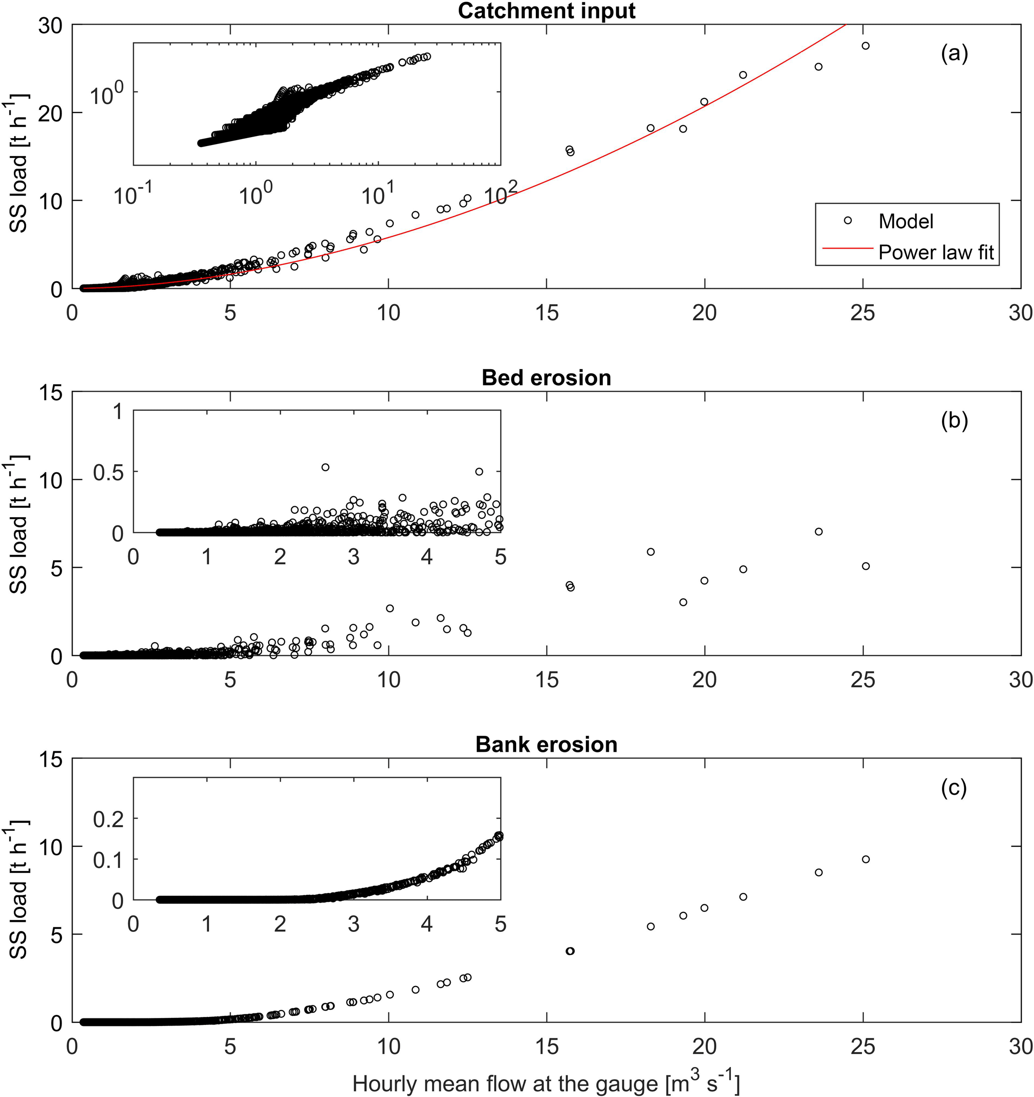
Figure 8Relationship between simulated hourly mean flow and hourly suspended-sediment loads from the catchment (a), bed erosion (b), and bank erosion (c), in which bed erosion and bank erosion are sums over all computation cells. Loads from the catchment are the sum of contributions from urban areas, nonurban areas, and the karst system.
As discussed above, we used a simplified approach to simulate the average sediment delivery from rural areas in our study because the contribution of rural areas to sediment delivery was so small. In particular, we did not distinguish between different crop types and seasons and estimated the average sediment load that reaches the streams instead. In other catchments, where the rural contributions to the sediment load are considerably higher, the description of soil erosion processes would require more differentiations.
To identify seasonal variations of suspended sediment loads originating from different processes, we used the model results of 2014–2016 to analyze the monthly mean suspended sediment loads from the urban areas, rural areas, the karst system, bed erosion, bank erosion, and deposition (Fig. 7). More suspended-sediment loads from urban areas and at the gauge can be observed in June and July (summer months). In summer months events with high rain intensity are more common than in winter months, which results in higher discharge peaks, more sediments generated in urban areas, and higher suspended-sediment loads at the gauge. Monthly suspended-sediment loads at the gauge have similar dynamics as the monthly urban particle contributions. The suspended-sediment load from the karst system is higher in winter months because the subsurface flow in the Ammer catchment is higher in winter months. Rural particles contribute to the overall particle flux only during a few months because annual precipitation and rainfall intensity were relatively small, so that surface runoff generated from rural areas was also low.
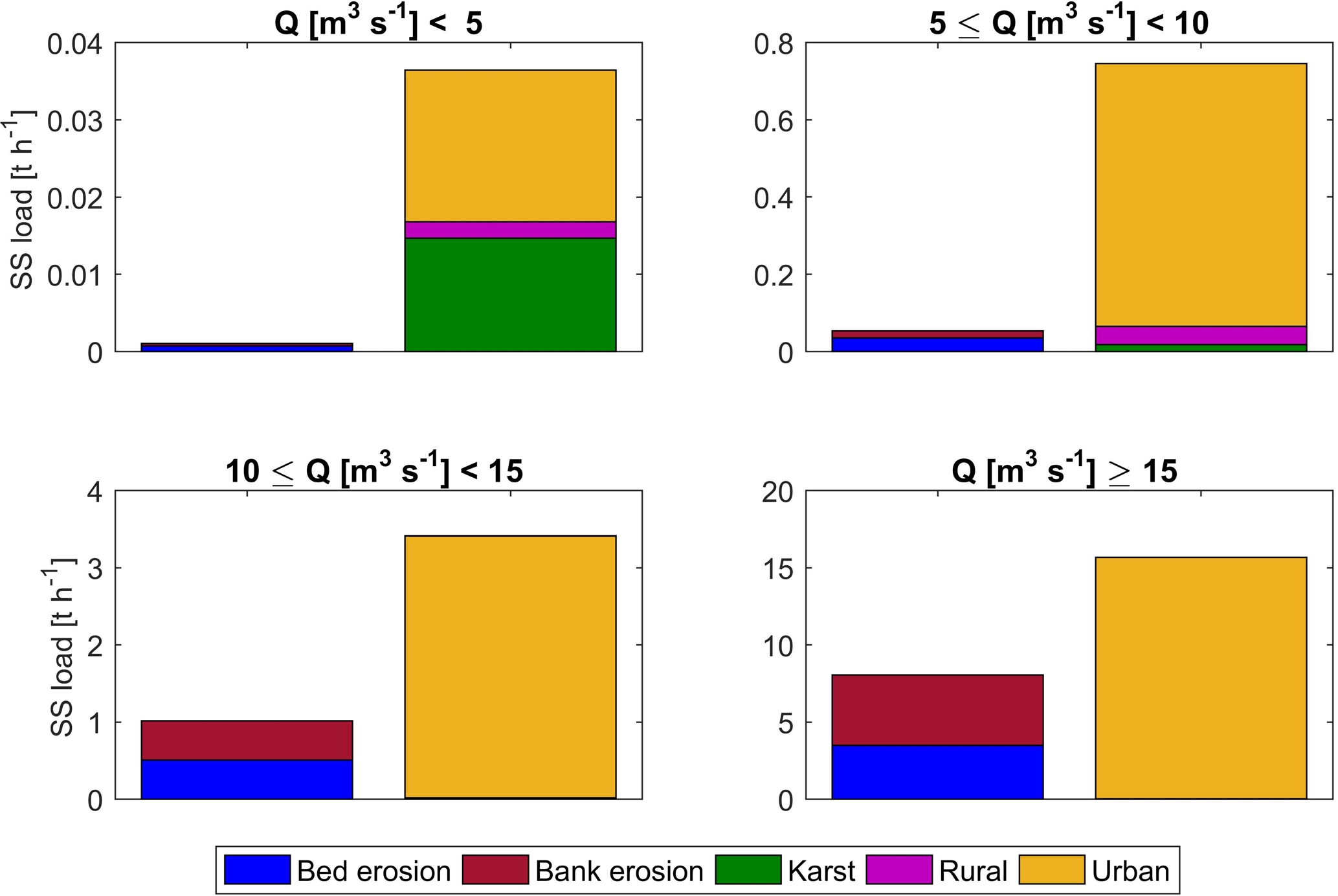
Figure 9Simulated suspended sediment load from bed erosion, bank erosion, the karst system, rural areas, and urban areas (including suspended sediment from WWTPs) under different flow regimes, the suspended sediment loads are the mean values for the specific flow regimes.
In the model simulation period, the seasonal patterns of bed erosion and bank erosion are obvious. High bed erosion and bank erosion occur from June to August due to increased bed shear occurring during big events. The area above the line of Loadgauge indicates net deposition, which shows small variations with a slight increase in July and August. The slight increase in summer is due to increased suspended-sediment concentrations during summer months. Comparing monthly mean bed erosion and deposition shows that bed erosion was greater than deposition in July, which indicates that accumulated bed sediment can be partly eroded in July.
Table 4Summary of suspended-sediment sources under different flow conditions.
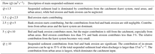
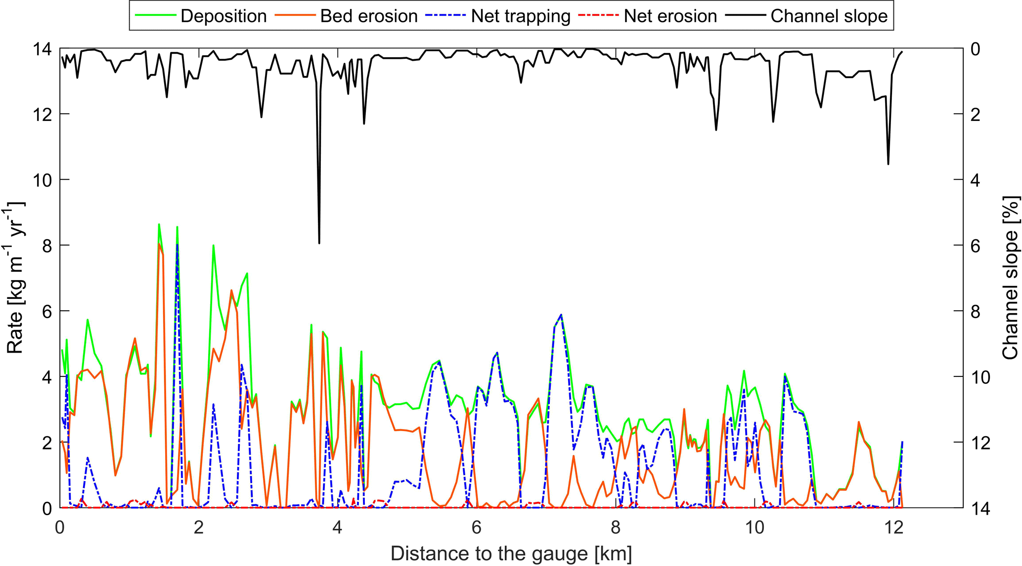
Figure 10The distribution of the annual mean deposition, bed erosion, net sediment trapping, net sediment erosion, and channel slope along the main channel of the Ammer River (flow direction from right to left). The blue and red dash–dotted lines highlight net sediment trapping and net erosion, respectively.
4.3 Suspended-sediment sources under different flow conditions
Figure 8 shows the relationship between hourly mean discharge and the simulated hourly suspended sediment loads from the catchment, bed erosion, and bank erosion. The hourly suspended-sediment load from the catchment monotonically increases with increasing hourly mean discharge by a power-law relationship (Fig. 8a), which is consistent with the particle wash-off rate being a power-law function of discharge. Bed erosion requires that the bed shear stress exceeds a critical value, so that bed erosion is almost 0 when hourly mean flow is smaller than 1.5 m3 s−1, namely 1.5 times mean discharge (Fig. 8b). For discharge larger than this threshold (1.5 m3 s−1), bed erosion increases approximately linearly with discharge. The simulated hourly bed-erosion loads for a given flow rate vary substantially because bed erosion is not only influenced by the shear stress, which directly depends on discharge, but also on the bed sediment storage, which depends on previous deposition and erosion events. Bank erosion occurs when the hourly mean flow rate is larger than 2.5 m3 s−1, i.e., 2.5 times mean discharge (Fig. 8c). The relationship between bank-erosion-related loads and discharge is more unique than that of bed-erosion loads because we assume an infinite source for bank erosion.
Figure 9 shows the suspended sediment loads from in-stream (bed erosion and bank erosion) and catchment processes (input from the karst system, urban areas, and rural areas) under different flow regimes. The fractions of suspended-sediment contributions from different processes change with flow regimes. The contributions of in-stream processes are negligible in the flow regime of discharge smaller than 5 m3 s−1. With the discharge increasing, the contributions of in-stream processes increase. The in-stream processes play significant roles in high-flow regimes, which contribute 23 and 34 % of total suspended sediment loads under flow regimes of 10≤Q (m3 s−1) < 15 and Q (m3 s−1) ≥15, respectively. The relative contribution of the karst system is high in the low-flow regime (Q < 5, in m3 s−1, while it can be neglected under high-flow regimes (Q > 10, in m3 s−1). With the increase in flow rates, the contribution of urban particles becomes dominant in terms of catchment processes, especially when discharge is larger than 10 m3 s−1.

Figure 11Monthly mean bed erosion along the channel of the Ammer River upstream of the gauge (flow direction from right to left).
From above observations, we can see that the sources of suspended sediments differ under different flow conditions in the following way (Table 4):
4.4 Hotspots and hot moments of bed erosion in the Ammer River
The annual mean rates of bed erosion and deposition (mass per unit length per year) along the main channel can be used to identify hotspots of bed erosion and net sediment trapping (Fig. 10). The rates of deposition and bed erosion vary substantially along the main stem, ranging from essentially zero to a maximum of 8.6 and 8.0 kg m yr−1, respectively. Bed erosion is higher in the river segment close to the gauge because the flow rate is higher due to the contributions of the tributaries. Bed erosion is rather low in the river segments within 5–6.5, 7–8, 8.5–9, and 10–11 km to the gauge, where the channel slope is very mild. The river sections with the steepest channel slope typically do not show the highest bed erosion because there is not enough sediment available for erosion, which is caused by insufficient deposition. Figure 10 also shows that when the channel slope is very mild, the deposition rate is very high, while the bed erosion rate is nearly zero. These are sections where net sediment trapping (blue dash–dotted line) was observed. With increasing channel slope, bed erosion rates increase and deposition rates decrease. In a small range of channel slopes, deposition rates equal to erosion rates, resulting in a local steady state. If the channel slope continues to increase, the erosion rate will be higher than the deposition rate, which results in net sediment erosion if the sediment storage in the channel is large enough (red dash–dotted line, very few in Fig. 10). Where the channel slope is very steep, both sediment deposition and erosion rates are very small.
Figure 11 shows monthly means of the bed erosion rates along the Ammer main stem, computed for the simulated years 2014 to 2016. Bed erosion is stronger in the summer months, especially in July, which is consistent with the monthly load of suspended sediments discussed in Sect. 4.2. The hot moments of bed erosion are the extreme events caused by summer thunderstorms. The downstream river segments close to the gauge show higher bed erosion rates than the sections further upstream because flow rates and thus bed shear stresses are higher even with identical channel slope.
Suspended sediment transport is of great importance for river morphology, water quality, and aquatic ecology. In this study, we have presented an integrated sediment-transport model, combining a conceptual hydrological model with a river-hydraulics model, a model of sediment generation, and a shear-stress-dependent sediment-transport model within the river, which enables us to investigate the major contributors to the suspended-sediment loads in different river sections under different flow conditions.
In the dominantly groundwater-fed Ammer catchment, annual suspended-sediment load is dominated by the contributions of urban particles and sediment input from the karst system. The contribution from rural areas is small because the topography is comparably flat and the infiltration capacity of the soils is high in this region, resulting in a very weak surface runoff from rural areas, and thus very few rural particles are generated and transported to the river channel. In-stream processes, i.e., bed erosion and bank erosion, play significant roles in high-flow conditions (Q > 10 m3 s−1). The flow rate governs the contributions of different processes to the suspended sediment loads. In particular, bed erosion and bank erosion take place when flow rates reach the corresponding thresholds, 1.5 and 2.5 times the mean discharge, respectively. The channel slope has significant effects on the deposition and bed erosion rates. Net sediment trapping was found in the river segments with very mild channel slopes in the Ammer River during the simulation period with events of a 2-year to 10-year return period. Finally, the river hydraulics model is necessary to differentiate sediment sources and sinks of in-stream processes, i.e., shear-stress-related deposition, bed erosion, and bank erosion.
The model and results of this study are useful and essential for further research on the fate and sediment-facilitated transport of hydrophobic pollutants like PAHs, and for the design of optimal sampling regimes to capture the different processes that drive particle dynamics. In addition, the analysis of deposition and bed erosion in the Ammer main stem provides information on the distribution of net sediment trapping within the channel, which would be a good indicator that channel dredging improves water quality.
The full code, as well as the supporting information related to this article, is provided in the Supplement.
The hydrological model in the integrated sediment transport model is composed of three storage zones in vertical direction with a quick recharge component and an urban surface runoff component. Detailed processes are shown below.
We applied this model to 14 subcatchments of the study domain. Each subcatchment includes three different land uses: urban area, agriculture, and forest. For urban areas, we consider effective urban areas such as roads and roofs and ineffective urban areas such as parks and gardens. We use the same parameters of agriculture for ineffective urban area.
The effective urban area is used for surface runoff component, the ratio is calculated by the following:
in which reff (–) is the ratio of effective urban area over total urban area, and Aeff (km2) and Aurb (km2) represent areas of effective urban area and total urban area, respectively.
The effective precipitation to the subsurface storage for agriculture, forest, and ineffective urban area is calculated below:
in which Pe (mm d−1) indicates effective precipitation, P (mm d−1) is precipitation, SM (mm) and FC (mm) are soil moisture and maximum soil storage capacity, respectively, and α (–) is a shape factor.
We use long-term monthly mean evapotranspiration to calculate the actual evapotranspiration with a temperature adjustment.
in which Let (mm) is a threshold for maximum evapotranspiration, and cet (–) is a factor to calculate Let. ETt (mm d−1) represents the maximum evapotranspiration at temperature T (∘C). ETm (mm d−1) and Tm (∘C) indicate long-term monthly mean evapotranspiration and long-term monthly mean temperature, respectively, and ct (∘C−1) is a temperature adjustment factor. ETa (mm d−1) represents actual evapotranspiration, which reaches maximum evapotranspiration when soil moisture is greater than the threshold for maximum evapotranspiration. Otherwise, it increases linearly with soil moisture.
The top storage layer, soil moisture, is calculated by the following:
in which (mm d−1) represents the change rate of soil moisture. It is used for agriculture and forest. The change rate of soil moisture for urban areas is , because we assume that precipitation in the effective urban areas will directly become urban surface runoff.
The surface runoff in the effective urban area, overflow and interflow are calculated by the following:
in which qeffurb (mm d−1) is surface runoff in the effective urban area, and qof (mm d−1) represents overflow when subsurface storage Sup (mm) is greater than an overflow threshold Lof (mm). It is used for agriculture, forest, and ineffective urban areas. The term qif (mm d−1) represents interflow, kif (d−1) is a rate constant, qbf (mm d−1) represents base flow, Sgw (mm) is groundwater storage, and kbf (d−1) is a base-flow recession coefficient.
The two equations below are used to calculate percolation and quick recharge.
in which qperc (mm d−1) represents percolation from soil moisture to subsurface storage; kperc (d−1) is a rate constant; qqr (mm d−1) represents quick recharge, which occurs when subsurface storage reaches a quick recharge threshold Lqr (mm); and kqr (d−1) is a rate constant.
The subsurface storage and groundwater storage are calculated by:
in which (mm d−1) is the change rate of subsurface storage. In the urban area, only precipitation in the ineffective area can partly become recharge to the subsurface storage. The term (mm d−1) represents the change rate of groundwater storage.

Figure A1The hydrological model for the Ammer catchment with three storage zones (soil moisture, subsurface storage, and groundwater storage), a quick groundwater recharge and an urban surface runoff component.
The supplement related to this article is available online at: https://doi.org/10.5194/hess-22-3903-2018-supplement.
YL, CZ, NBB, and OAC conceptualized the study. YL wrote the code with the help of OAC. MS provided and preprocessed the data of discharge and turbidity. YL prepared the paper and all co-authors were involved in reviewing the paper.
The authors declare that they have no conflict of interest.
This study was supported by the German Research Foundation (Deutsche
Forschungsgemeinschaft, DFG) within the Research Training Group “Integrated
Hydrosystem Modeling” (grant GRK 1829). Additional funding is granted by the
Collaborative Research Center SFB 1253 “CAMPOS – Catchments as Reactors”,
and by the EU FP7 Collaborative Project GLOBAQUA (grant agreement no.
603629).
Edited by: Christian Stamm
Reviewed by: two anonymous referees
Amalfitano, S., Corno, G., Eckert, E., Fazi, S., Ninio, S., Callieri, C., Grossart, H.-P., and Eckert, W.: Tracing particulate matter and associated microorganisms in freshwaters, Hydrobiologia, 800, 145–154, https://doi.org/10.1007/s10750-017-3260-x, 2017.
Bicknell, B. R., Imhoff, J. C., Kittle Jr., J. L., Jobes, T. H., and Donigian Jr., A. S.: HYDROLOGICAL SIMULATION PROGRAM – FORTRAN, Version 12, AQUA TERRA Consultants, California, US, 2001.
Bilotta, G. S. and Brazier, R. E.: Understanding the influence of suspended solids on water quality and aquatic biota, Water Res., 42, 2849–2861, https://doi.org/10.1016/j.watres.2008.03.018, 2008.
BKG: Spatial Data Access Act of 10 February 2009, Federal Law Gazette [BGBl.] Part I, p. 278,, Bundesamt für Kartographie und Geodäsie (BKG), 2009
Bones, E. J.: Predicting critical shear stress and soil erodibility classes using soil properties, Georgia Institute of Technology, 2014.
Bouchaoua, L., Manginb, A., and Chauve, P.: Turbidity mechanism of water from a karstic spring: example of the Ain Asserdoune spring (Beni Mellal Atlas, Morocco), J. Hydrol., 265, 34–42, 2002.
Bouteligier, R., Vaes, G., and Berlamont, J.: Sensitivity of urban drainage wash-off models: compatibility analysis of HydroWorks QM and MouseTrapusing CDF relationships, J. Hydroinform., 4, 235–243, 2002.
Brunner, G. W.: HEC-RAS, River Analysis System Hydraulic Reference Manual Version 5.0, Institute for Water Resources Hydrologic Engineering Center, Davis, CA US, 2016.
BwAm: Weather data at weather station Bondorf, Agrarmeteorologie Baden-Württenmberg (BwAm), 2016.
CDC: Historical hourly station observations of precipitation for Germany, version v005, DWD Climate Data Center (CDC), 2017.
Clark, L. A. and Wynn, T. M.: Methods for determining streambank critical shear stress and soil erodibility: Implications for erosion rate predictions, T. ASABE, 50, 95–106, 2007.
Dong, J., Xia, X., Wang, M., Lai, Y., Zhao, P., Dong, H., Zhao, Y., and Wen, J.: Effect of water–sediment regulation of the Xiaolangdi Reservoir on the concentrations, bioavailability, and fluxes of PAHs in the middle and lower reaches of the Yellow River, J. Hydrol., 527, 101–112, https://doi.org/10.1016/j.jhydrol.2015.04.052, 2015.
Dong, J., Xia, X., Wang, M., Xie, H., Wen, J., and Bao, Y.: Effect of recurrent sediment resuspension-deposition events on bioavailability of polycyclic aromatic hydrocarbons in aquatic environments, J. Hydrol., 540, 934–946, https://doi.org/10.1016/j.jhydrol.2016.07.009, 2016.
Ferro, V. and Porto, P.: Sediment Delivery Distributed (Sedd) Model, J. Hydrol. Eng., 5, 411–422, https://doi.org/10.1061/(Asce)1084-0699(2000)5:4(411), 2000.
Flanagan, D. C. and Nearing, M. A.: USDA – WATER EROSION PREDICTION PROJECT, USDA-ARS National Soil Erosion Research Laboratory, Indiana, US, 1995.
Gilley, J. E., Elliot, W. J., Laflen, J. M., and Simoanton, J. R.: Critical Shear Stress and Critical Flow Rates for Initiation of Rilling, J. Hydrol., 142, 251–271, 1993.
Gong, Y., Liang, X., Li, X., Li, J., Fang, X., and Song, R.: Influence of Rainfall Characteristics on Total Suspended Solids in Urban Runoff: A Case Study in Beijing, China, Water, 8, 278, 1–23, https://doi.org/10.3390/w8070278, 2016.
Grabowski, R. C., Droppo, I. G., and Wharton, G.: Erodibility of cohesive sediment: The importance of sediment properties, Earth-Sci. Rev., 105, 101–120, https://doi.org/10.1016/j.earscirev.2011.01.008, 2011.
Hanson, G. J. and Simon, A.: Erodibility of cohesive streambeds in the loess area of the midwestern USA, Hydrol. Process., 15, 23–38, 2001.
Haygarth, P. M., Bilotta, G. S., Bol, R., Brazier, R. E., Butler, P. J., Freer, J., Gimbert, L. J., Granger, S. J., Krueger, T., Macleod, C. J. A., Naden, P., Old, G., Quinton, J. N., Smith, B., and Worsfold, P.: Processes affecting transfer of sediment and colloids, with associated phosphorus, from intensively farmed grasslands: an overview of key issues, Hydrol. Process., 20, 4407–4413, https://doi.org/10.1002/hyp.6598, 2006.
Kaase, C. T. and Kupfer, J. A.: Sedimentation patterns across a Coastal Plain floodplain: The importance of hydrogeomorphic influences and cross-floodplain connectivity, Geomorphology, 269, 43–55, https://doi.org/10.1016/j.geomorph.2016.06.020, 2016.
Krone, R. B.: Flume studies of the transport of sediment in estuarial shoaling processes, Univ. of Calif., Berkeley, 1962.
Léonard, J. and Richard, G.: Estimation of runoff critical shear stress for soil erosion from soil shear strength, Catena, 57, 233–249, https://doi.org/10.1016/j.catena.2003.11.007, 2004.
LGRB: Bodenkarte von Baden-Württemberg 1 : 50 000, GeoLa – Integrierte Geowissenschaftliche Landesaufnahme, Regierungspräsidium Freiburg Landesamt für Geologie, Rohstoffe und Bergbau, 2011.
Lindström, G., Johansson, B., Persson, M., Gardelin, M., and Bergström, S.: Development and test of the distributed HBV-96 hydrological model, J. Hydrol., 201, 272–288, 1997.
LUBW: Erstellung von Hochwassergefahrenkarten des Landes Baden-Württemberg, LUBW (Landesanstalt für Umwelt, Messungen und Naturschutz, Karlsruhe), 2010.
Meus, P., Moureaux, P., Gailliez, S., Flament, J., Delloye, F., and Nix, P.: In situ monitoring of karst springs in Wallonia (southern Belgium), Environ. Earth Sci., 71, 533–541, https://doi.org/10.1007/s12665-013-2760-x, 2013.
Meyer, T. and Wania, F.: Organic contaminant amplification during snowmelt, Water Res., 42, 1847–1865, https://doi.org/10.1016/j.watres.2007.12.016, 2008.
Modugno, M., Gioia, A., Gorgoglione, A., Iacobellis, V., Forgia, G., Piccinni, A., and Ranieri, E.: Build-Up/Wash-Off Monitoring and Assessment for Sustainable Management of First Flush in an Urban Area, Sustainability, 7, 5050–5070, https://doi.org/10.3390/su7055050, 2015.
Morgan, R. P. C., Quinton, J. N., Smith, R. E., Govers, G., Poesen, J. W. A., Auerswald, K., Chisci, G., Torri, D., and Styczen, M. E.: The European Soil Erosion Model (EUROSEM): A dynamic approach for predicting sediment transport from fields and small catchments, Earth Surf. Proc. Land., 23, 527–544, https://doi.org/10.1002/(Sici)1096-9837(199806)23:6<527::Aid-Esp868>3.0.Co;2-5, 1998.
Mukherjee, D. P.: Dynamics of metal ions in suspended sediments in Hugli estuary, India and its importance towards sustainable monitoring program, J. Hydrol., 517, 762–776, https://doi.org/10.1016/j.jhydrol.2014.05.069, 2014.
Neitsch, S. L., Arnold, J. G., Kiniry, J. R., and Williams, J. R.: Soil and Water Assessment Tool, Theoretical Documentation Version 2009, Texas Water Resources Institute, Texas A&M University System, Texas, US, 2011.
Partheniades, E.: Erosion and Deposition of Cohesive Soils, J. Hydr. Eng. Div., 91, 105–139, 1965.
Patil, S., Sivapalan, M., Hassan, M. A., Ye, S., Harman, C. J., and Xu, X.: A network model for prediction and diagnosis of sediment dynamics at the watershed scale, J. Geophys. Res., 117, F00A04, https://doi.org/10.1029/2012jf002400, 2012.
Peraza-Castro, M., Sauvage, S., Sanchez-Perez, J. M., and Ruiz-Romera, E.: Effect of flood events on transport of suspended sediments, organic matter and particulate metals in a forest watershed in the Basque Country (Northern Spain), Sci. Total Environ., 569–570, 784–797, https://doi.org/10.1016/j.scitotenv.2016.06.203, 2016.
Piro, P. and Carbone, M.: A modelling approach to assessing variations of total suspended solids (tss) mass fluxes during storm events, Hydrol. Process., 28, 2419–2426, https://doi.org/10.1002/hyp.9809, 2014.
Romero, C. C., Stroosnijder, L., and Baigorria, G. A.: Interrill and rill erodibility in the northern Andean Highlands, Catena, 70, 105–113, https://doi.org/10.1016/j.catena.2006.07.005, 2007.
Quesada, S., Tena, A., Guillen, D., Ginebreda, A., Vericat, D., Martinez, E., Navarro-Ortega, A., Batalla, R. J., and Barcelo, D.: Dynamics of suspended sediment borne persistent organic pollutants in a large regulated Mediterranean river (Ebro, NE Spain), Sci. Total Environ., 473–474, 381–390, https://doi.org/10.1016/j.scitotenv.2013.11.040, 2014.
Quinton, J. N. and Catt, J. A.: Enrichment of Heavy Metals in Sediment Resulting from Soil Erosion on Agricultural Fields, Environ. Sci. Technol., 41, 3495–3500, 2007.
Rossman, L. A. and Huber, W. C.: Storm Water Management Model, Reference Manual, Volume III – Water Quality, US Environmental Protection Agency, Cincinnati, OH, US, 2016.
Rügner, H., Schwientek, M., Beckingham, B., Kuch, B., and Grathwohl, P.: Turbidity as a proxy for total suspended solids (TSS) and particle facilitated pollutant transport in catchments, Environ. Earth Sci., 69, 373–380, https://doi.org/10.1007/s12665-013-2307-1, 2013.
Rügner, H., Schwientek, M., Egner, M., and Grathwohl, P.: Monitoring of event-based mobilization of hydrophobic pollutants in rivers: calibration of turbidity as a proxy for particle facilitated transport in field and laboratory, Sci. Total Environ., 490, 191–198, https://doi.org/10.1016/j.scitotenv.2014.04.110, 2014.
Scanlon, T. M., Kiely, G., and Xie, Q.: A nested catchment approach for defining the hydrological controls on non-point phosphorus transport, J. Hydrol., 291, 218–231, https://doi.org/10.1016/j.jhydrol.2003.12.036, 2004.
Schwientek, M., Osenbrück, K., and Fleischer, M.: Investigating hydrological drivers of nitrate export dynamics in two agricultural catchments in Germany using high-frequency data series, Environ. Earth Sci., 69, 381–393, 10.1007/s12665-013-2322-2, 2013a.
Schwientek, M., Rugner, H., Beckingham, B., Kuch, B., and Grathwohl, P.: Integrated monitoring of particle associated transport of PAHs in contrasting catchments, Environ. Pollut., 172, 155–162, https://doi.org/10.1016/j.envpol.2012.09.004, 2013b.
Selle, B., Schwientek, M., and Lischeid, G.: Understanding processes governing water quality in catchments using principal component scores, J. Hydrol., 486, 31–38, https://doi.org/10.1016/j.jhydrol.2013.01.030, 2013.
Siddiqui, A. and Robert, A.: Thresholds of erosion and sediment movement in bedrock channels, Geomorphology, 118, 301–313, https://doi.org/10.1016/j.geomorph.2010.01.011, 2010.
Slaets, J. I. F., Schmitter, P., Hilger, T., Lamers, M., Piepho, H.-P., Vien, T. D., and Cadisch, G.: A turbidity-based method to continuously monitor sediment, carbon and nitrogen flows in mountainous watersheds, J. Hydrol., 513, 45–57, https://doi.org/10.1016/j.jhydrol.2014.03.034, 2014.
UBA: CORINE Land Cover (CLC2006), Umweltbundesamt (German Environmental Protection Agency) (DLR-DFD 2009), 2009.
Wicke, D., Cochrane, T. A., and O'Sullivan, A.: Build-up dynamics of heavy metals deposited on impermeable urban surfaces, J. Environ. Manage., 113, 347–354, https://doi.org/10.1016/j.jenvman.2012.09.005, 2012.
Winterwerp, J. C., van Kesteren, W. G. M., van Prooijen, B., and Jacobs, W.: A conceptual framework for shear flow-induced erosion of soft cohesive sediment beds, J. Geophys. Res.-Oceans, 117, C10020, https://doi.org/10.1029/2012jc008072, 2012.
Wischmeier, H. and Smith, D. D.: Predicting rainfall erosion losses, USDA Science and Education Administration, 1978.
Zhang, M. and Yu, G.: Critical conditions of incipient motion of cohesive sediments, Water Resour. Res., 53, 7798–7815, https://doi.org/10.1002/2017WR021066, 2017.
Zhang, Y., Xiao, W., and Jiao, N.: Linking biochemical properties of particles to particle-attached and free-living bacterial community structure along the particle density gradient from freshwater to open ocean, J. Geophys. Res.-Biogeo., 121, 2261–2274, https://doi.org/10.1002/2016jg003390, 2016.