the Creative Commons Attribution 3.0 License.
the Creative Commons Attribution 3.0 License.
Scale effect challenges in urban hydrology highlighted with a distributed hydrological model
Abdellah Ichiba
Auguste Gires
Ioulia Tchiguirinskaia
Daniel Schertzer
Philippe Bompard
Marie-Claire Ten Veldhuis
Hydrological models are extensively used in urban water management, development and evaluation of future scenarios and research activities. There is a growing interest in the development of fully distributed and grid-based models. However, some complex questions related to scale effects are not yet fully understood and still remain open issues in urban hydrology. In this paper we propose a two-step investigation framework to illustrate the extent of scale effects in urban hydrology. First, fractal tools are used to highlight the scale dependence observed within distributed data input into urban hydrological models. Then an intensive multi-scale modelling work is carried out to understand scale effects on hydrological model performance. Investigations are conducted using a fully distributed and physically based model, Multi-Hydro, developed at Ecole des Ponts ParisTech. The model is implemented at 17 spatial resolutions ranging from 100 to 5 m. Results clearly exhibit scale effect challenges in urban hydrology modelling. The applicability of fractal concepts highlights the scale dependence observed within distributed data. Patterns of geophysical data change when the size of the observation pixel changes. The multi-scale modelling investigation confirms scale effects on hydrological model performance. Results are analysed over three ranges of scales identified in the fractal analysis and confirmed through modelling. This work also discusses some remaining issues in urban hydrology modelling related to the availability of high-quality data at high resolutions, and model numerical instabilities as well as the computation time requirements. The main findings of this paper enable a replacement of traditional methods of “model calibration” by innovative methods of “model resolution alteration” based on the spatial data variability and scaling of flows in urban hydrology.
- Article
(11640 KB) - Full-text XML
- BibTeX
- EndNote


Urban environments are very complex systems due to their intrinsic extreme variability over a wide range of spatio-temporal scales, and the interaction between human activities and natural processes. A notable illustration is the ongoing urbanization process that changes land cover and strongly influences the hydrological behaviour of urban catchments. Urban hydrological models were developed over the years and used to simulate the portion of the water cycle in urban environments (Refsgaard and Knudsen, 1996; Tech University of Darmstadt and Ostrowski, 2002; Salvadore et al., 2015; Hromadka, 1987; Daniel et al., 2011; Elliott and Trowsdale, 2007; Sarma et al., 1973; Blöschl and Sivapalan, 1995). They can be classified according to either the nature of the employed algorithms (empirical, conceptual or physically based; Salvadore et al., 2015), or their spatial resolution and how they represent the complexity of urban hydrology processes (lumped, semi-distributed and fully-distributed models).
Lumped (Kleidorfer et al., 2009) and semi-distributed (Insa-Valor, 1999) models are conceptual ones and rely on a simplified representation of urban catchment's heterogeneity. Indeed the whole catchment is considered as a single unit with homogeneous features for the lumped ones, while a catchment is divided into a limited number of homogeneous sub-catchments for the semi-distributed models. These two approaches were widely developed and used for modelling applications because they require limited amount of data for their implementation, and exhibit fast computation time. They often rely on a calibration step that '“forces” the model to represent the observed data. However, these models give output information at the sub-catchment scale, which is too coarse for meeting urban water managers' requirements in their need to understand some very local flooding problems or to evaluate management strategies at very small scales. Hence, the need has arisen to change the spatial resolution of hydrological models, and several works in the literature have investigated this approach for semi-distributed models (Park et al., 2008; Stephenson, 1989). It appears that the aggregation and disaggregation of sub-catchments changes the model output, which reflects a “scale effect issue”, and that the complex calibration step must be performed again to obtain performance similar to the previous configuration.
The influence of catchment scale on hydrological response is more pronounced for fully distributed (Ichiba, 2016) and gridded-based models, because of their modelling approach that usually consists in representing the high heterogeneity of urban catchment in a gridded format. The choice of an appropriate spatial resolution is always critical and the obtained model performance strongly depends on the chosen implementation scale (Ichiba, 2016). The appropriate spatial resolution is obviously linked to the quality and resolution of data available as well as the modelling goal (Dehotin and Braud, 2008). A more accurate representation of the land cover heterogeneity is obtained using a high-resolution grid (small pixel size). However, given current computational capabilities and data availability, high-resolution modelling is feasible only for small areas. Therefore, it is important for modellers to understand the effects of spatial resolution in urban hydrological simulations.
Scale effects and scaling in urban hydrology have been investigated by researchers – for example Gires et al. (2013); Park et al. (2008); Stephenson (1989); Elliott et al. (2009); Wood et al. (1988); Zhang and Montgomery (1994). This topic was also reviewed by Blöschl and Sivapalan (1995). Ostrowski (2002) discussed temporal and spatial scaling issues in the context of urban storm water modelling. Dehotin and Braud (2008) proposed a spatial discretization methodology applied for distributed hydrological models to get an efficient representation of land cover heterogeneity. Ghosh and Hellweger (2012) investigated the effects of spatial resolution on predictions of peak flow and total outflow volume in an urban catchment. Zhang and Montgomery (1994) analysed the Digital Elevation Model (DEM) grid size and land cover representation. They found that the effect of grid size on the model performance is not linear; a 10 m grid size provides a substantial improvement over 30 and 90 m data, whereas 2 or 4 m data provide only marginal additional improvement. Wood et al. (1988) investigated the effects of scale in urban hydrology by trying to identify a threshold scale called “Representative Elementary Area (REA)”. The REA is strongly influenced by the topography.
Fractal tools will be used in this work to characterize scale effects in environmental data. They are widely used in several science domains including geology, medicine, meteorology and finance (Niu et al., 2016; West, 2012; Goldberger and West, 1987; Nonnenmacher et al., 2013; Turcotte and Huang, 1995; Yanshi and Kaixuan, 2002; Turcotte, 1989). In hydrology, the fractal dimension concept has been used in many studies in the past for various purposes, ranging from catchment geometrical characterization to flow analysis (Mesev et al., 1995; Wu et al., 2013; Thibault and Crews, 1995; Frankhauser, 1998; Wu and He, 2009; Sagar, 2004; Jiang et al., 2012; Gires et al., 2013; Radziejewski and Kundzewicz, 1997), but has seldom been used in urban hydrology (Gires et al., 2017).
This work was motivated by the fact that on the one hand the inputs of the hydrological models exhibit scale-invariant features while on the other hand distributed models are implemented at a single resolution. Hence the question we seek to investigate in this paper is “at which resolution should we implement the model?” – bearing in mind practical constraints such as missing data at high resolution or longer computation time. The main goal of the paper is to investigate the existence and try to identify the appropriate resolution (or a range of resolution) for a Multi-Hydro model (Sect. 3) implementation over a peri-urban area close to Paris (Sect. 4). We first use fractal tools to analyse the features of the model's inputs and then we perform multi-scale modelling work. Methodology is presented in Sect. 4 and results are discussed in Sect. 5.
Multi-Hydro (Fig. 1, Multi-Hydro, 2015; Giangola-Murzyn, 2013; Ichiba, 2016; El Tabach et al., 2009) is a fully distributed and physically based model developed at Ecole des Ponts ParisTech which has been used by several authors (Ichiba, 2016; Giangola-Murzyn, 2013; Versini et al., 2016; Gires et al., 2014). It is an interacting core between four open source software packages, each of them representing a portion of the water cycle in urban environments. Multi-Hydro involves a modelling approach that consists in rasterizing the urban domain at a specific spatial resolution chosen by the user. A unique land use class for which hydrological and physical properties are specified is then assigned to each pixel.
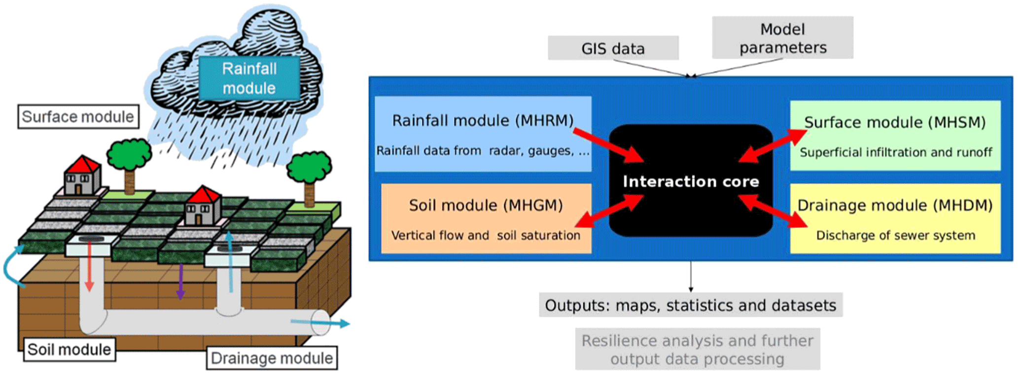
Figure 1The Multi-Hydro model is an interacting core between four modules, each of them representing a portion of the water cycle in urban environments. © (Giangola-Murzyn, 2013).
The modelling approach involved in Multi-Hydro model relies on solving physical equations that describe the catchment behaviour. Seven processes are generally simulated; (1) precipitation, (2) interception and storage, (3) infiltration, (4) overland flow, (5) sewer flow, (6) infiltration into the subsurface zone and (7) sewer overflow.
The four modules that make up the core of Multi-Hydro are presented in Fig. 1:
-
The surface component (MHSC) is based on the existing TREX model (Two-dimensional Runoff, Erosion, and Export model) developed by Colorado State University and used in Multi-Hydro only for rainfall–runoff modelling (Velleux et al., 2008). The surface module computes interception, storage and infiltration occurring at each pixel according to the properties of its land cover class. The overland flow can occur after exceeding the depression storage threshold, and it is governed by equations ensuring the conservation of mass (continuity) and momentum. This flow depends on the surface properties as well as the elevation, and is computed using the diffusive wave approximation of Saint-Venant equations (England et al., 2007; Velleux et al., 2008).
-
The rainfall module was developed at Ecole des Ponts ParisTech. It is used to manage different types of rainfall data (rain gauges, radar data,…) and to process them in the correct input format needed for the Multi-Hydro model. The module also performs some data analysis and can be used for radar data downscaling. The downscaling and data analysis carried out relies on the multifractal framework (Lovejoy and Schertzer, 1990; Schertzer and Lovejoy, 1987) and has been used in an urban context by Gires et al. (2012).
-
The Drainage module (MHDC) is based on the 1-D SWMM (James et al., 2010) model (Storm Water Management Model) developed by the US Environmental Protection Agency. It is widely used for urban drainage and modelling purposes. The flow in the sewer network is given by a numerical solution of Saint-Venant equations. This module requires a detailed description of the sewer network (nodes, pipes characteristics, gullies, outlet…).
-
The infiltration module relies on the VS2DT model developed by the US Geological Survey. It is used to simulate the infiltration into the unsaturated subsurface zone (Healy, 1990; Lappala et al., 1987). This module uses the infiltration depth calculated by the surface module as input, and simulates a 2D infiltration (vertical and 1-D horizontal) into the subsurface. This module was not used here because the analysis of the subsurface infiltration was not one of the objectives of this work.
The four modules are connected via the Multi-Hydro core, which groups together a set of codes allowing interaction, retro-action (feedback) and data exchange between these modules. In this case study, these interactions are performed after each time loop of 5 min. More precisely, the surface module outputs are used as inputs for the soil and the drainage modules, and in the same way the sewer overflow is taken into account in the overland depth for the next step. Multi-Hydro produces a large set of outputs that describe the catchment response. For example, overland water depth maps are available at each time step as well as overland discharge flow maps and velocity profiles at any point of the catchment. Saturation profile of the subsurface zone and sewer flows are also computed. The model also provides a detailed volume balance at each time step.
Multi-Hydro is highly demanding on data quality and resolution. Distributed data (usually available in GIS format) describing the topography and land use over the catchment must be collected at a high resolution. Precise information about all the components of the sewer network are also necessary for the drainage module. Such information is usually available for urban areas and can be obtained from the local authority in charge of the water management. Details about all pipes (geometry, length, diameter as well as inlet and outlet nodes) should be carefully validated, as well as all the system nodes (coordinates and elevation). The subsurface structure should be described as well if there is a need to simulate the infiltration through the unsaturated zone. The rasterization of the urban domain is the first step of Multi-Hydro implementation. During this process a unique class of land use is attributed to each individual pixel. This attribution can be done following at least two methodologies, illustrated in Fig. 2. The first one is based on a priority order defined by the user to attribute land use class. The second method is based on a majority rule, which means that each pixel will be affected by the majority class of land observed within it, with an exception of the gully class which remains a priority regardless of the method applied, to ensure the connection between the surface and the drainage system.
The possibility to implement other rules was investigated in the framework of Ichiba (2016), but the model formulation allows only one land use class (characterized by a few parameters such as the conductivity) per pixel. This means that implementing other approaches (such as a fractional approach) would require to a great increase in the number of classes as well as the development of a multifractal spatial characterization of key parameters such as conductivity. Those are possible motivating future investigation paths but they are outside the scope of the current study. Hence it was chosen to limit the study to two rules for affecting pixels' class, while keeping the number of classes reasonable.
The two rules considered here were tested and compared by Ichiba (2016). The main findings are reported in Sect. 5 (see Figs. 12 and 13) and indicate that considering the majority rule methodology leads to a better representation of the catchment heterogeneity. Consequently, the majority rule was used here during the rasterization step to attribute a unique land cover class to each pixel.

Figure 2Two attribution methodologies are implemented in Multi-Hydro and can be used during the rasterization phase. The first one is based on a priority order defined by the user to attribute land use class, whereas the second methodology is based on a majority rule. In both methodologies, the gully class has priority, to ensure the connection between the surface and the drainage modules.
Multi-Hydro has already been implemented in several locations for different purposes: in the cities of Villecresnes (France) and Manchester (UK) for flood mitigation by using barriers and retention basins (Giangola-Murzyn, 2013), in Sucy (France) for retention basin management (Ichiba, 2016), in Sevran (France) to study the impact of small-scale rainfall variability in urban areas (Gires et al., 2014), and in Villepinte and Champs-sur-Marne (France) for quantifying the impact of large-scale implementation of blue and green infrastructures on storm water management (Versini et al., 2016).
3.1 Sucy-en-Brie catchment
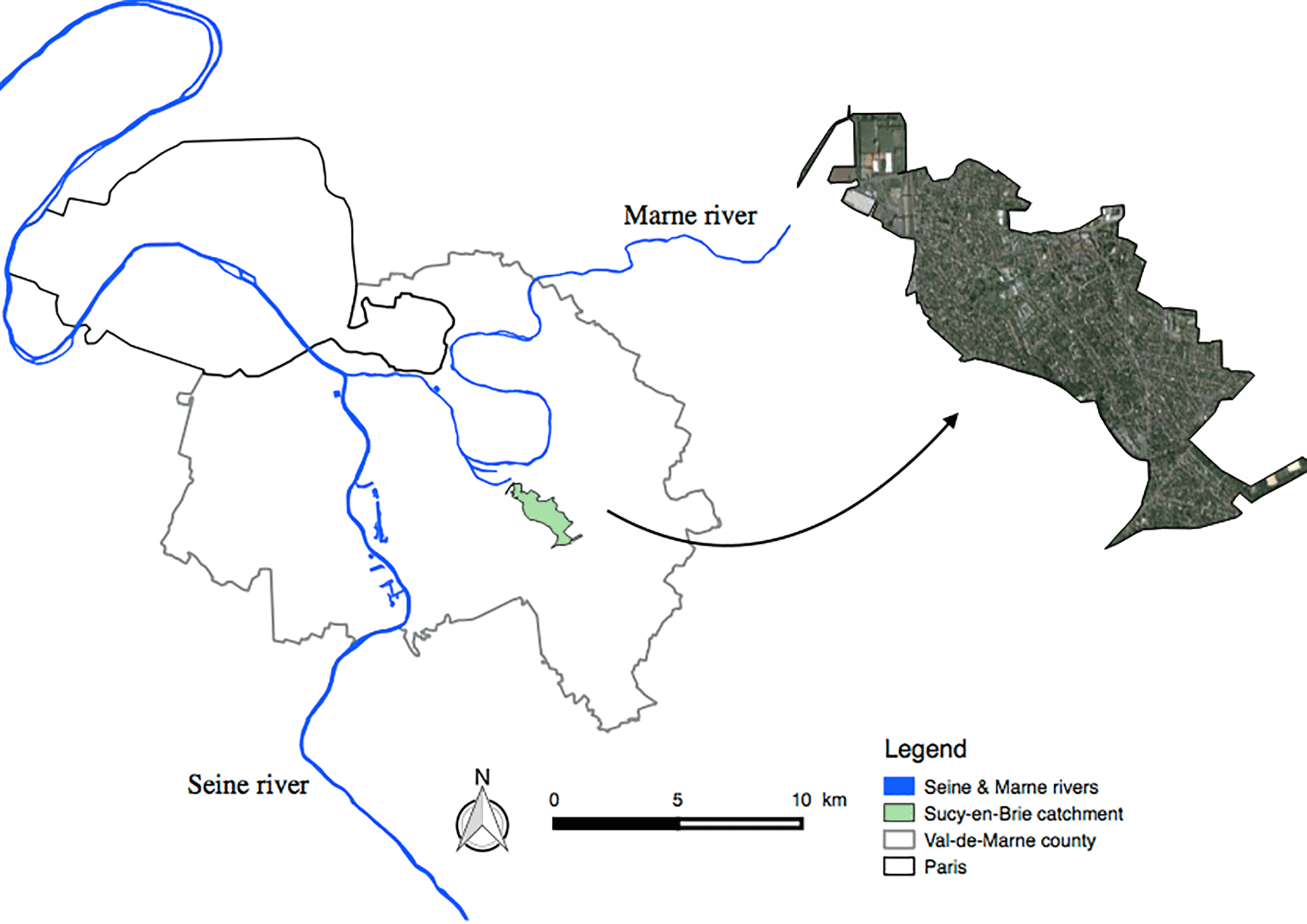
The case study presented in this paper is a 2.45 km2 urban catchment located southeast of Paris, in Val-de-Marne County, which is part of the Île-de-France region (Fig. 3). The city is connected to Paris via a train at the Sucy-Bonneuil station (30 min travel time to the centre of Paris). Known historically as an agriculture area, the city is now highly urbanized with an imperviousness coefficient around 35 %. The city is bounded at the north by the Marne river (one of the two main rivers in the Paris region). The area has suffered in the past from several flooding events as a consequence of (1) the very steep slope (34 m km−1) that increases water speed and causes overflows in the downstream portion of the storm water network and (2) the increase of impervious areas combined with a soil structure that limits infiltration to the subsurface. The drainage system in this area is a separated one (i.e. there are separate networks for waste water and storm water). The storm water system is routed to the Marne River.
3.2 Distributed data
Spatially distributed data are used in this study to set up the Multi-Hydro model. The data were made available by various public institutions in the framework of research collaborations with Ecole des Ponts ParisTech.
-
Topography: the Digital Elevation Model (DEM) of the catchment was obtained from the IGN (French National Institute of Forest and Geographic Information). The spatial resolution of the data is 25 m with a 1 m resolution in height, which is far from meeting the needs of the studies carried out in this work. Linear interpolation was implemented to obtain data at a better resolution (between 5 and 10 m).
-
Land cover: Fig. 4 shows distributed data (available in GIS format) describing the land cover. The data were obtained from the DSEA 94 of Val-de-Marne County (Direction des Services de l'Environnement et de l'Assainissement). Its quality is high, with a precision of up to 50 cm, but we had to deal with one land use class named ”Other” in the original data. This class corresponds to unknown information and introduces missing data. A comparison with satellite images was done and the majority of missing data was filled with urban grass.
-
Sucy-en-Brie subsurface structure: the subsurface structure was elaborated using data obtained from the BRGM database (Office of Geological and Mining Research) from soil investigations done before construction works and archived in the BRGM database. The data indicate that a layer of clay mixed in some places with sand dominates the majority of the catchment subsurface. Downstream, near the river, there is a layer of sandy soil which is much more permeable. Physical parameters characterizing soil, which are needed for modelling, were obtained from the literature (Lappala et al., 1987) and no measurements were done to verify or to estimate these parameters.
-
Sucy-en-Brie storm runoff system: the sewer system in this catchment (Fig. 5) is a separate one. The storm water system is routed downstream to the Marne river. The DSEA 94 of Val-de-Marne County is the service in charge of the control and the management of the whole system. Data describing the sewer system in this area are very detailed, consisting of 2030 nodes and 1015 elements of pipes representing a total length of 25 km. The average slope is around 0.052 m m−1.
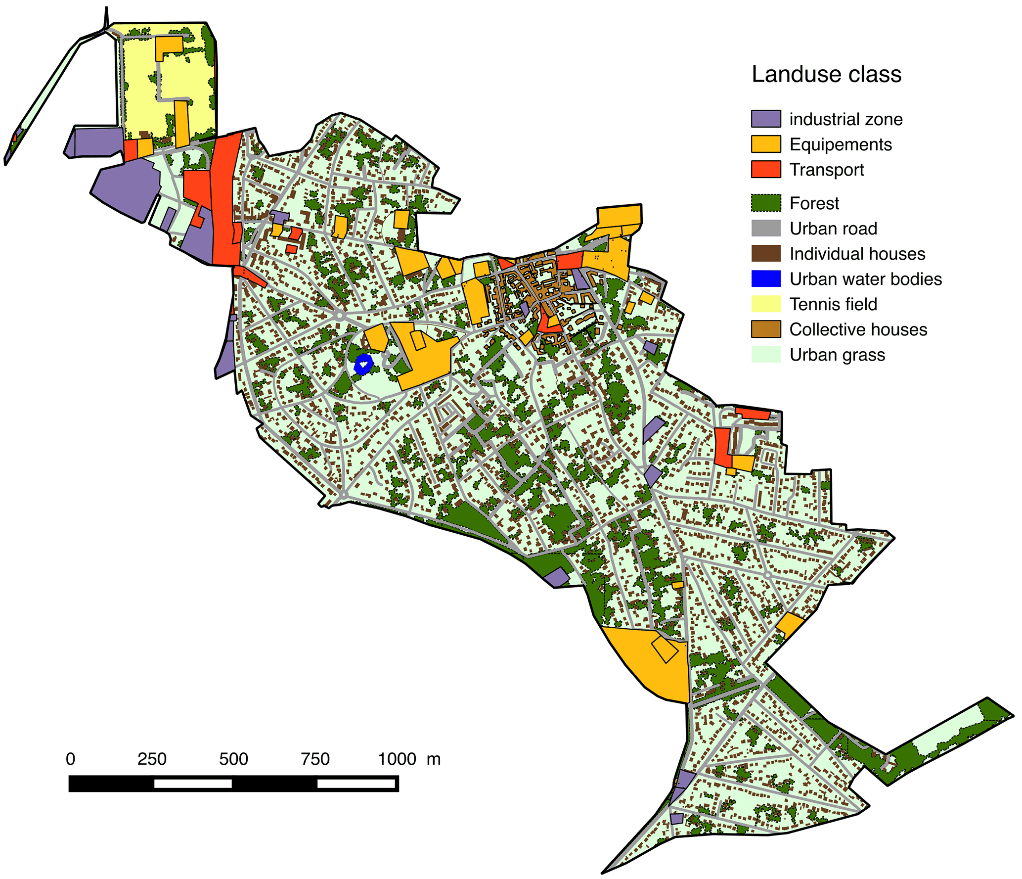
Figure 4The land cover data available for Sucy-en-Brie catchment and used to implement the Multi-Hydro model.
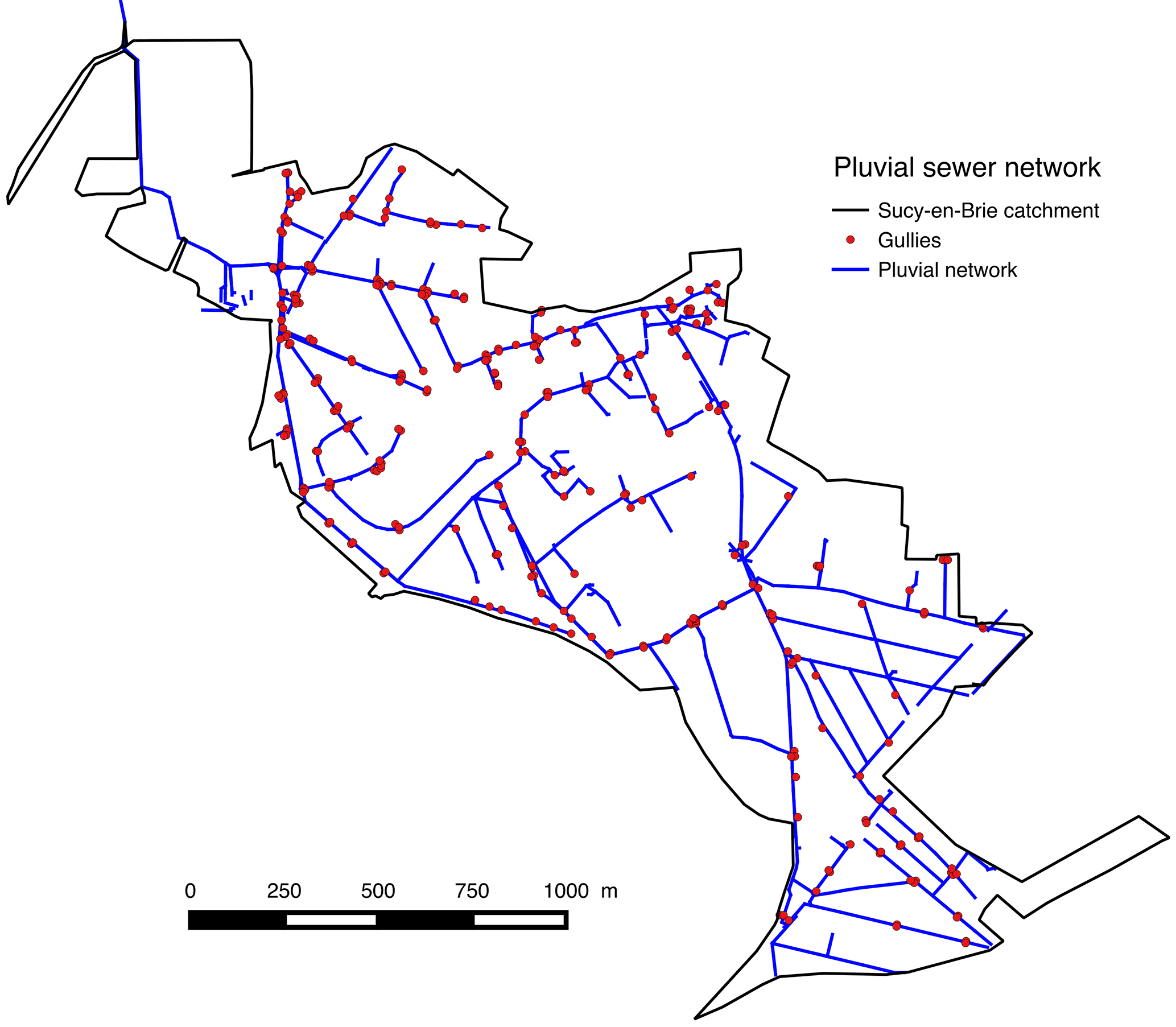
Figure 5The storm water system of Sucy-en-Brie catchment which is used to implement the Multi-Hydro model.
3.3 Rainfall and flow measurements data
Rainfall data are provided by the General Council of Val-de-Marne County. The data come from a 0.2 mm resolution tipping bucket rain gauge located at the centre of the catchment. The data were processed and validated by the DSEA 94 and provided with a 5 min resolution. Eight rainfall events (Fig. 6) that occurred between 2010 and 2014 were selected. Their main characteristics are summarized in Table 1. The corresponding flow measurement data were available, also at 5 min resolution – coming from a flow sensor located at the outlet of the catchment. The choice was made in this work to use uniform rainfall information in order to focus on the sensitivity of the Multi-Hydro model to land use variability and to avoid the effect of rainfall spatial variability.
Table 1Main characteristics of the eight rainfall events selected to perform the scale dependence investigations. Imax is the maximum rainfall intensity recorded in mm h−1 over 5 min.
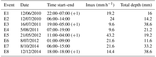
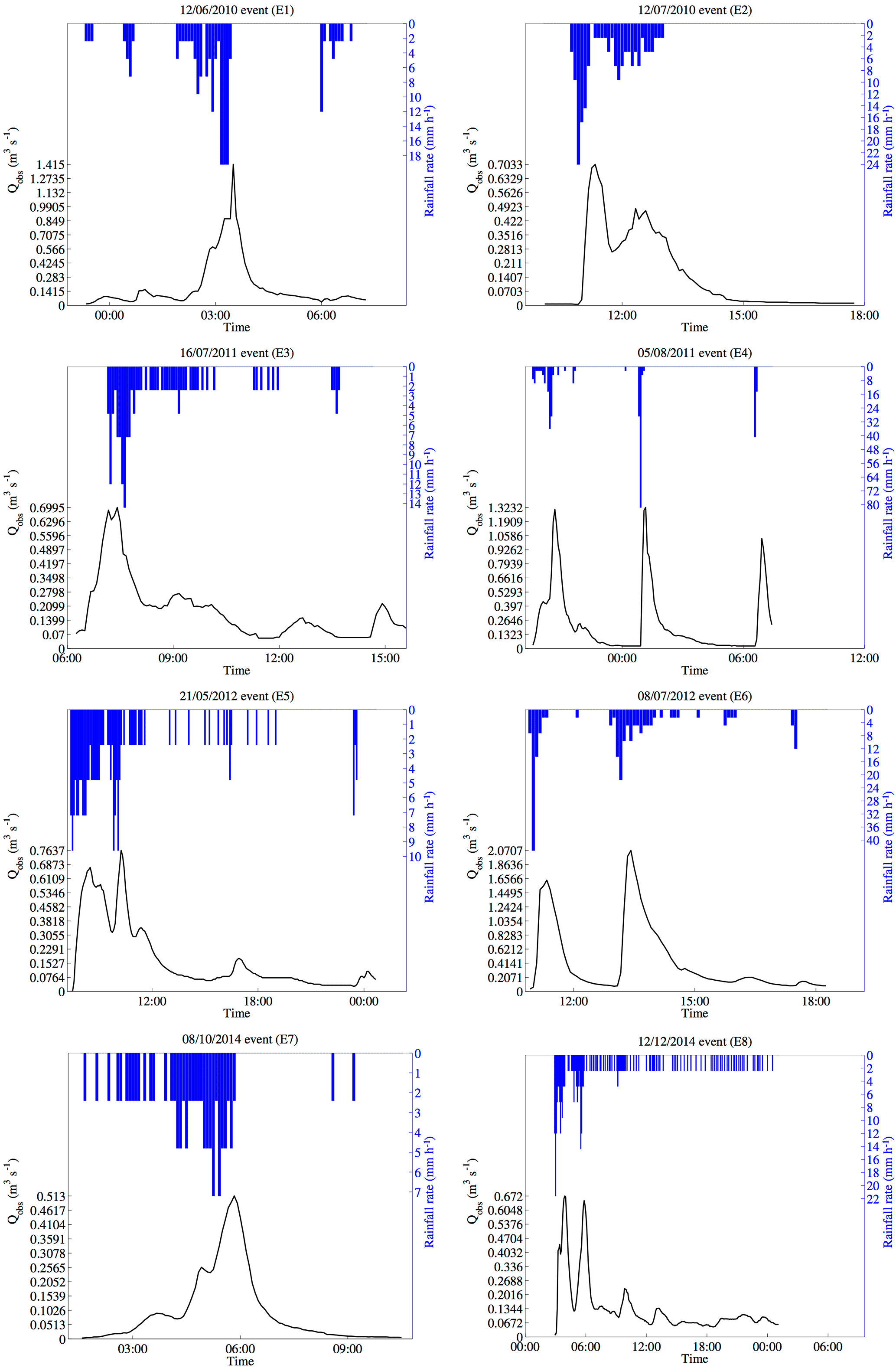
Figure 6Rainfall data and the corresponding flow measurement available for the eight rainfall events selected to perform the multi-scale modelling investigation.
4.1 Part 1: analysis of the scaling of urban catchment
The first step of this work is to investigate and identify the scale dependence observed within the distributed GIS information (presented in Sect. 3.2) used as input for hydrological models. The analysis relies on the fractal dimension concept.
Fractal geometry was formally introduced by Mandelbrot (1983) and is used to describe geometrical sets that exhibit a great level of complexity, i.e. they are too irregular to be easily described with the help of basic Euclidean concepts but they can be described with the help of simple and iterative processes. Fractal sets exhibit scale invariance, which means that similar structure will be observed at any scale. The concept of fractal dimension is used to characterize them. The fractal dimension Df is the exponent of the power-law relation between the resolution λ, which is defined as the ratio between the outer scale l0 and the observation scale l (), and the number of non-overlapping pixels Nλ,A needed to cover the set (A) at a given resolution:
Hence Df is the asymptotic slope of Nλ,A vs. λ in a log-log plot. It has a limit behaviour, meaning that mathematically the fractal dimension is defined as follows:
Figure 7 shows an example of how fractal analysis is practically implemented in urban hydrology to analyse a portion of the sewer system. Several pixel sizes are used to cover the sewer network starting from 2 m pixels and multiplying their size by 2 at each step. The number of pixels Nλ needed at a given resolution λ to cover the storm water system is computed and plotted in a log-log plot as a function of the resolution λ (blue points). Figure 7 shows the linear behaviour retrieved over two separate ranges of scales. This means that the concept of fractal dimension can be used to characterize the sewer network, but two regimes must be taken into account. In this work, the structure of the urban storm water system and the distribution of impervious land use will be analysed using fractal tools.
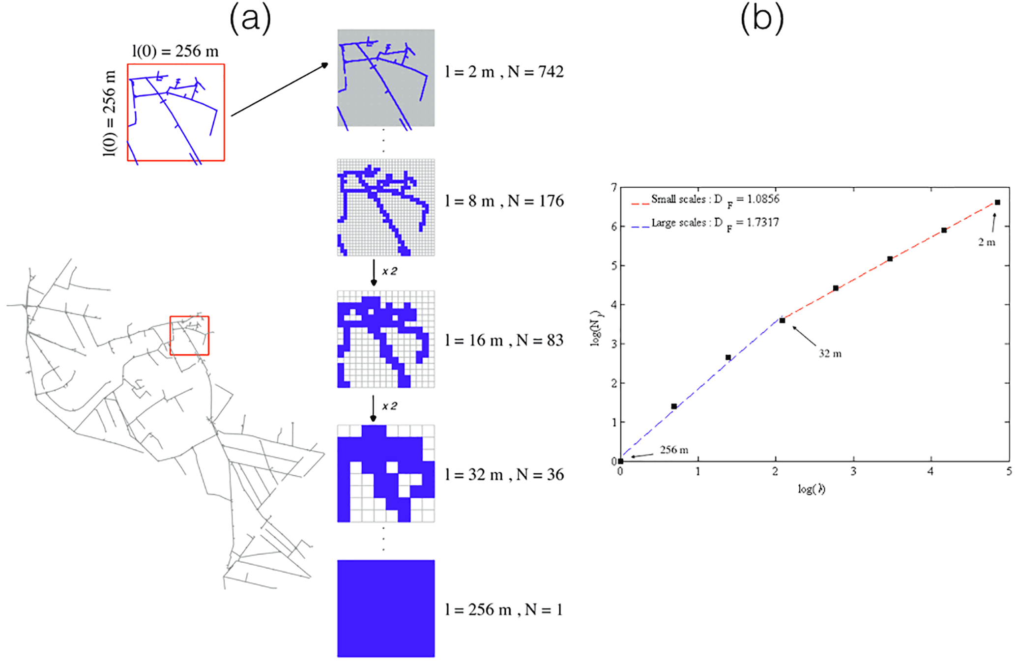
Figure 7Example of fractal analysis of a portion of the sewer network (256 m size). (a) Nλ is plotted as function of λ in a log-log plot. (b) A scaling behaviour is retrieved over two separate ranges of scales with a break around 32 m.
4.2 Part 2: scale effects on fully distributed models outputs
To address the effects of spatial resolution on Multi-Hydro performance, the model was implemented at 17 spatial scales ranging from 100 to 5 m and intensive modelling work was carried out. Figure 8 shows how the chosen grid size influences the way that land cover heterogeneity is represented in the model. These scale effects will be analysed with respect to real flow measurements from various points of view according to the performance indicators chosen:
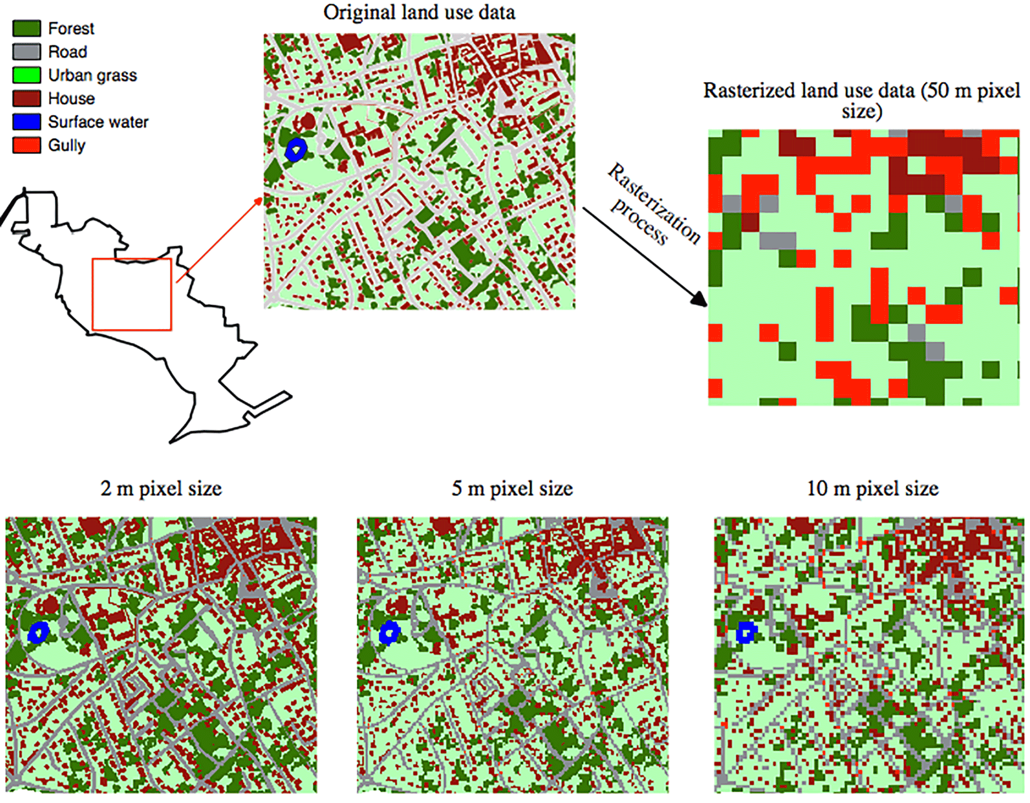
Figure 8Scale effect observed on the catchment land cover. The grid size strongly affects the way land cover heterogeneity is represented in the model.
-
Correlation coefficient r: The correlation coefficient r (Eq. 3) measures the strength and the direction of the linear relationship between the modelled flow Qmod and the observed one Qobs. It is computed as follows:
where cov(Qmod,Qobs) refers to the covariance of the variables Qmod and Qobs, and σmod and σobs are their respective standard deviations.
The r value ranges from −1 to +1. A positive value of r indicates that the two time series describe the same dynamic (they increase and decrease at the same moment). Generally, a correlation greater than 0.8 is described as strong, whereas a correlation smaller than 0.5 is described as weak.
-
Nash–Sutcliffe efficiency NSE: The NSE coefficient (Eq. 4) is the most commonly used indicator to quantify performance of urban hydrological models. NSE measures how well the model outputs reproduce the observation outputs in comparison with a model that only uses the mean of the observed data. The NSE coefficient is computed as follows:
where and are respectively the observed and modelled flow at time step t, is the mean of observed flow and n is the length of the time series.
NSE ranges from −∞ to +1. A value of 1 indicates a perfect model, while a value of zero indicates performance no better than simply using the mean. A negative value corresponds to performance worse than using just the mean. The pros and cons of the NSE coefficient have been discussed in the literature, and many attempts have been made to improve it (Gupta et al., 2009).
-
The coefficient of regression β: The β (Eq. 5) is computed as follows:
where cov(Qmod,Qobs) is the covariance between Qmod and Qobs, and var(Qobs) is the variance of the observed flow Qobs.
The β is used here to distinguish spatial scales for which the model overestimates and those for which the model underestimates the observed flow. The β values range between −∞ and +∞ and a value of β=1 indicates an ideal match between the observed and simulated flows. If β<1, then the model is underestimating the observed flow, otherwise it is overestimating the observed flow.
-
Peak flow relative error δr: A special focus is given to peak flows. The relative error observed at the peak flow δr (Eq. 6) is used to address effects of scale changes on the modelled peak flow. δr is estimated as follows:
where and refer respectively to the maximum modelled flow and the maximum observed one.
In total, 136 simulations (17 spatial resolutions, 8 rainfall events) were run and results were analysed with the help of these statistics. The analysis will help to identify spatial resolutions for which the model exhibits good performance with respect to available flow measurements.
5.1 Fractal analysis of distributed data
5.1.1 Fractal dimension of urban sewer network
Two areas have been selected to perform the fractal analysis for the storm water system. The purpose of this selection is to minimize the effect of no data pixels by considering two well-covered square areas whose size is a power of 2. Figure 9 shows the 2 m pixel size original data available and the two selected zones. The small and great area are respectively of size 512 m ( m) and 1024 m (=210 m).
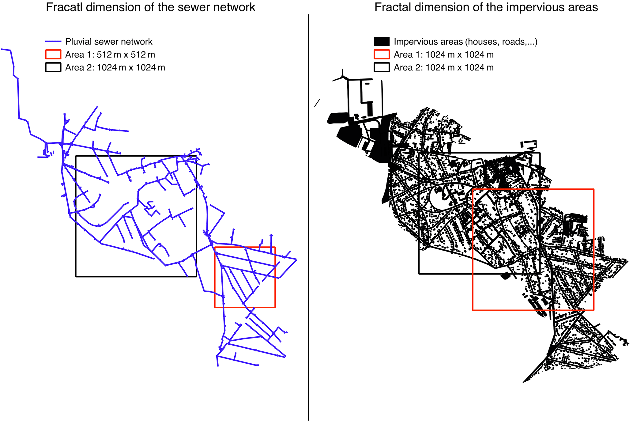
Figure 9The original 2 m pixel size data used to perform the fractal analysis of the storm water sewer system and impervious areas; two well-covered areas were selected.
Figure 10 displays results obtained when plotting in a log-log plot the number of pixels Nλ needed at a given resolution λ to cover the storm runoff system as a function of λ. Results show a clear agreement to the relation defined in Eq. (1) over two distinct ranges of scales separated by a break at ≈ 64 m. For small scales (2–64 m), the fractal dimension Df is almost equal to 1, simply reflecting the linear behaviour of the sewer pipes structure observed across this range scales. For large scales l≥ 64 m the fractal dimensions Df found of 1.82 and 1.88 are close to the dimension of the embedding space of 2. This means that over this range of scales, the structure of the pluvial networks fills most of the space. These results confirm similar conclusions of a multi-catchment work performed in the framework of the RainGain project about fractal analysis of environmental data of 10 pilot sites located in Europe (Gires et al., 2017). The break at 64 m is related, according to this study, to the typical distance between two roads in urban areas.
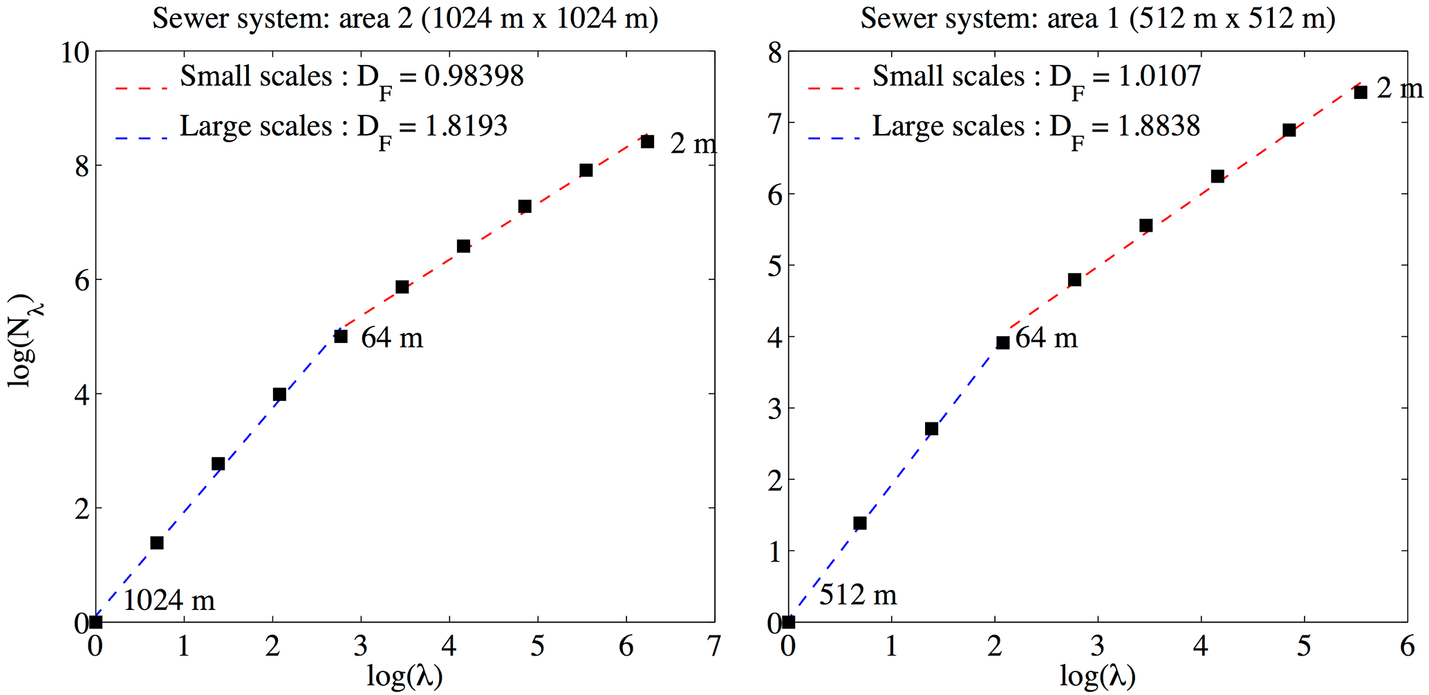
Figure 10Fractal analysis of the sewer system structure. Two ranges of scale are identified in both areas; Df is equal to 1 at small scales (2–64 m) and 1.8 for large scales l≥ 64 m.
5.1.2 Fractal dimension of impervious data
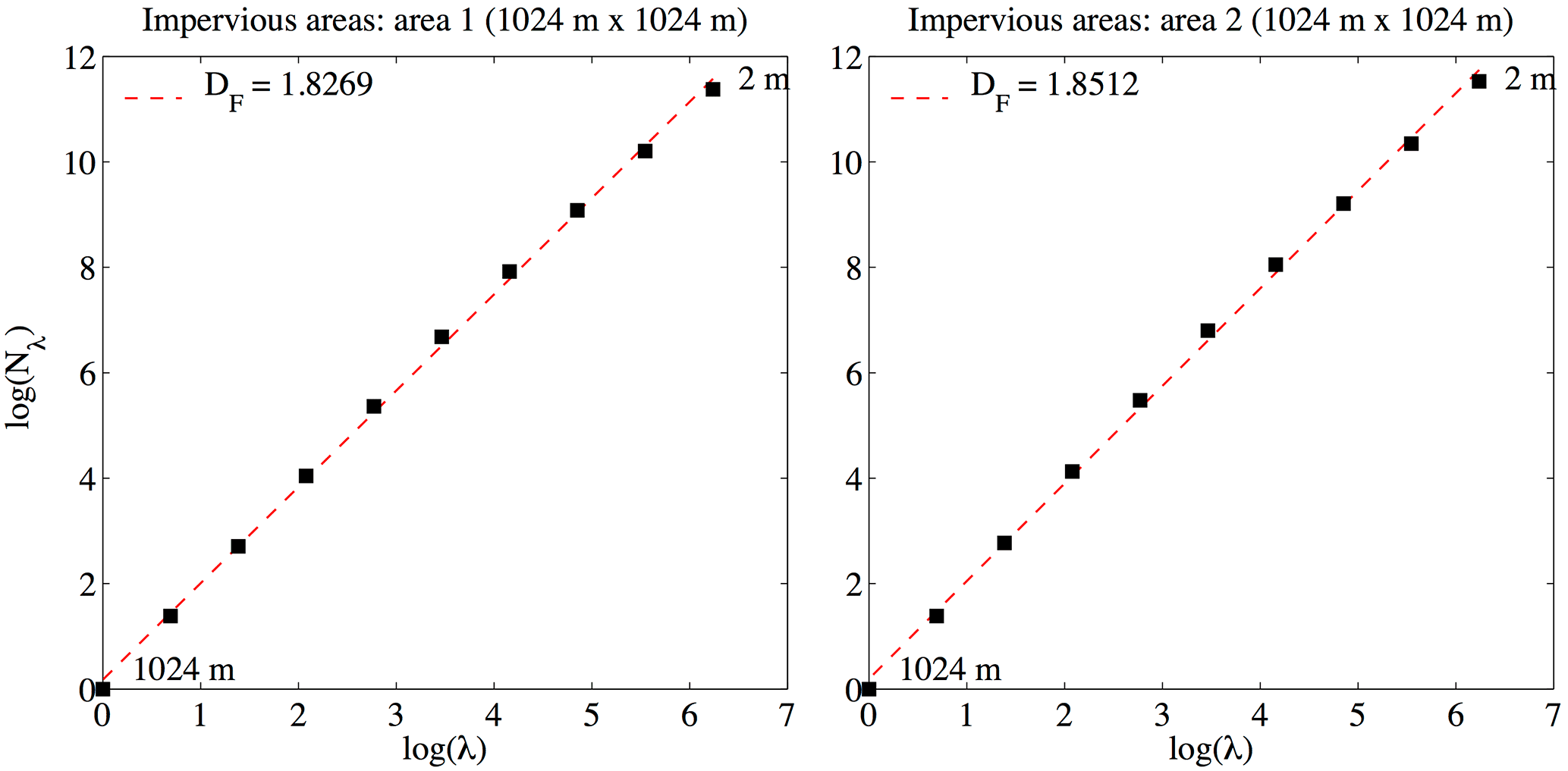
Figure 11Fractal analysis of the impervious data. One unique scaling regime is identified across the whole range of available scales (2–1024 m); Df is greater than 1.8 for both areas.
For impervious data (Fig. 9), two 1024 m size square areas were selected to perform the fractal analysis. Figure 11 shows the obtained results. Both areas exhibit a clear and unique scaling regime across the whole range of available scales (2–1024 m). This shows the high scale dependence of urban catchment patterns and demonstrate how important it is to well represent urban catchment heterogeneity when using gridded models. This scale dependence has significant consequences on a hydrological model performance, as we will show. The fractal dimension Df computed is 1.82 for Area 1 and 1.85 for Area 2, which is similar to the values retrieved for the large scales of sewer systems found in other European cities (Gires et al., 2017).
5.1.3 Effect on the urban catchment behaviour
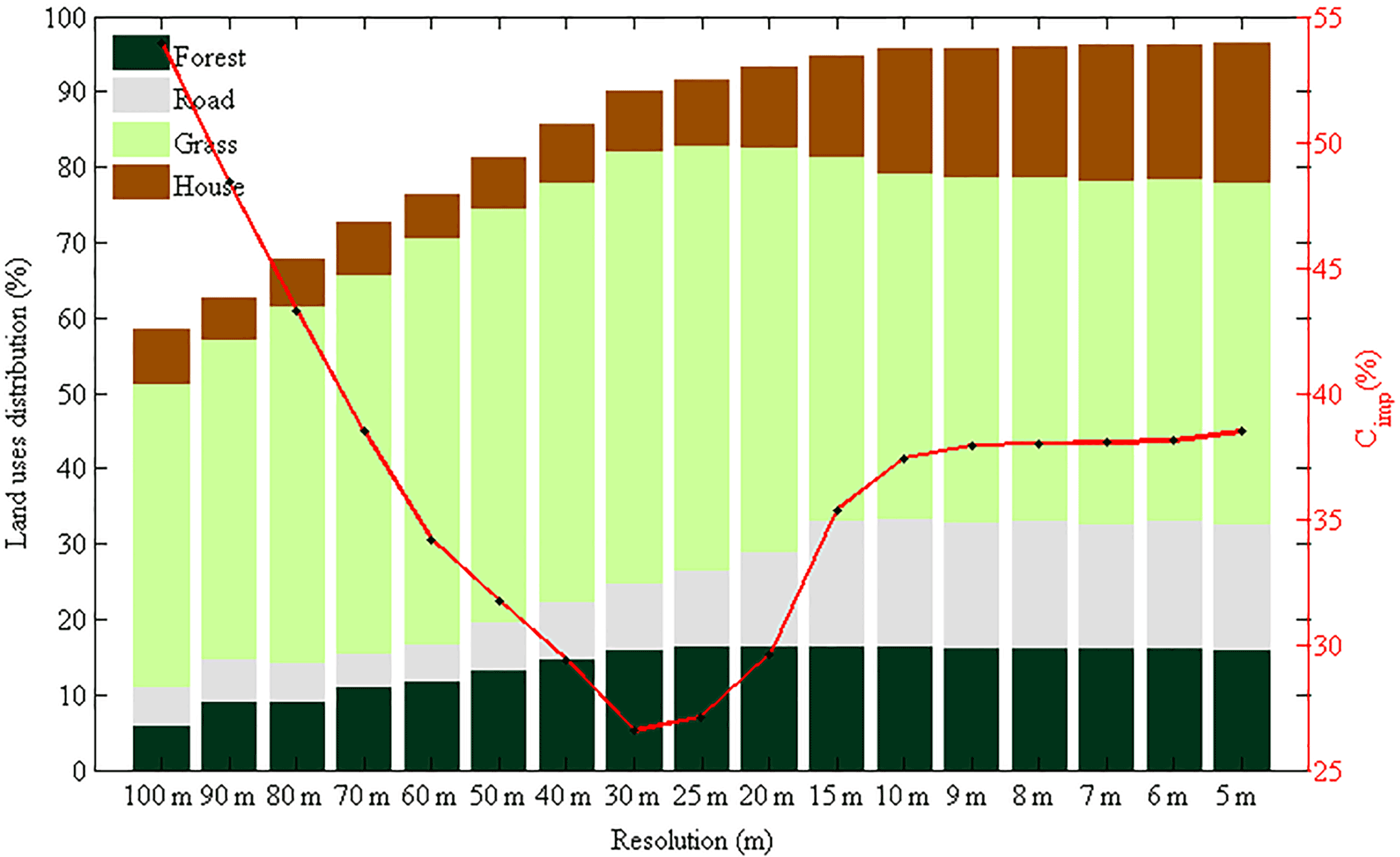
Previous results show that the urban catchment configuration considered in grid-based models highly depends on the scale at which the model is implemented. In fact, spatial patterns observed in the land cover strongly evolve with the observation scale. Figures 13 and 12 display, for the two land cover pixel attribution methodologies, the distribution of the four main land cover classes (forest, road, grass and house) considered in the Multi-Hydro model, as well as the imperviousness coefficient Cimp – defined as the ratio between impervious surface (gully, roads, houses) and the total surface – as a function of the model spatial scale. The imperviousness coefficient is actually not a parameter of the modelling formulation. It is simply a quantity used to gain some insight into the inputs of the model and how its overall features change with resolution. It refers here to the areas directly participating in the rapid runoff. Results with priority rule are in Fig. 12 and those obtained with the majority rule in Fig. 13.
Both figures demonstrate that the scale dependence highlighted here is mainly due to the rasterization methodology performed in the Multi-Hydro model during the implementation phase, which assigns a unique land cover to each pixel. At very small scales both methodologies will basically lead to the same catchment representation, whereas results obtained at intermediate scales are different. To illustrate these differences, let us consider the case of pixels of size 100 m. In an urban environment it is very likely that such a pixel will intersect a road. Then, with the priority rule, since “road” pixels have a high level of priority, this will make the portion of pixels affected by road land cover class greater. This portion decreases as the pixel size decreases. On the other hand, with the majority rule (Fig. 13), the portion of road pixels is smaller because the roads will usually not occupy the greater portion of such pixel.
The variation of the imperviousness coefficient Cimp (red line) provides an insight into the model behaviour across scales. It is continuously decreasing in the first configuration (Fig. 12), whereas in the second (Fig. 13), the behaviour is different. The high values of the Cimp coefficient at large scales are due to the fact that most of the priority land cover classes (gully, road and houses) are impermeable.
When applying the priority rule (Fig. 12), the imperviousness coefficient Cimp is still very high even at high resolution (5 m pixels), meaning that the user must perform hydrological simulations at much finer resolutions, which is challenging in urban hydrology modelling considering the quality of available GIS data, as well as computation time. On the other hand, Fig. 13 shows that the majority rule methodology is more suitable to take into account urban catchment heterogeneity at coarser resolutions. The land cover distribution is more coherent than with the previous methodology. In this case, three ranges of scales can be identified: (i) large scales (100–30 m) at which the imperviousness coefficient decreases significantly from 55 % observed at 100 m to its minimum value of 27 % at 30 m – this is due to a great redistribution of land cover classes; (ii) medium scales (30–10 m), at which the imperviousness coefficient increases from 27 to 37 % estimated at 10 m; (iii) small scales (10–5 m), at which we observe what can be considered as the final configuration of the catchment, i.e. the most accurate, and closer to the reality on the ground. Across small scales the imperviousness coefficient remains stable around 38 %, which suggests that the model response will be stable across this range of scales.
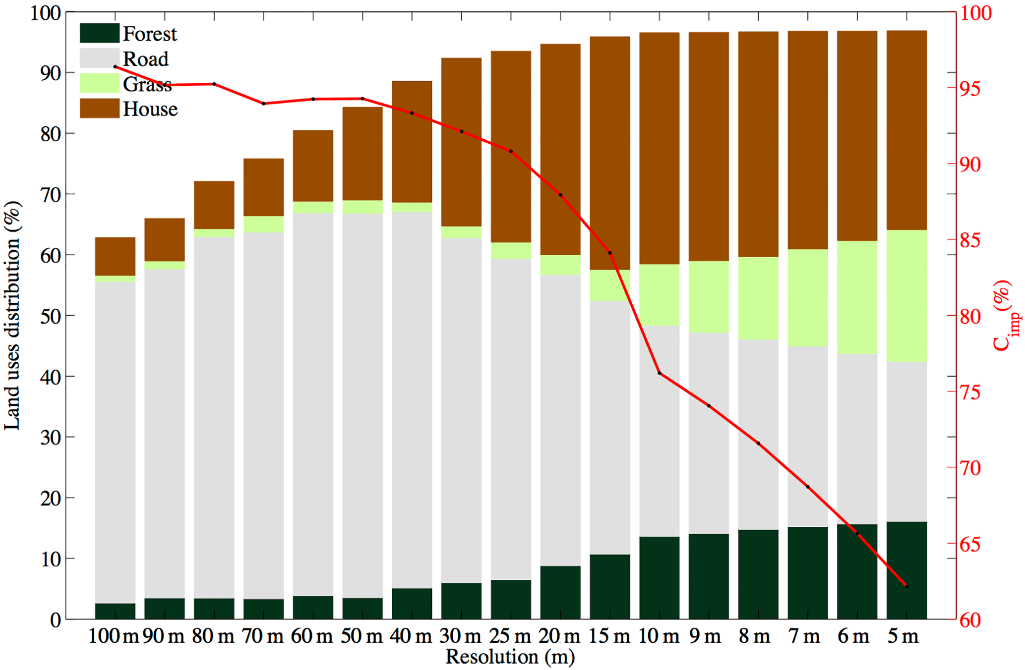
Figure 12Scale dependence observed in the overall distribution of land cover classes and the imperviousness coefficient Cimp with priority rule as explained in Fig. 2. The priority order was set as follows: gully, road, forest, house, grass.
5.2 Scale effects on Multi-Hydro model outputs
For each of the eight selected rainfall events, 17 simulations were carried out and the corresponding simulated flow time series were retrieved at the outlet pipe, where effects are typically smoothed compared to more upstream pipes.
Figure 14 represents all simulated flows Qs obtained with the Multi-Hydro model at the 17 spatial scales involved. These results show the high sensitivity of the outputs to the spatial scale of the model.
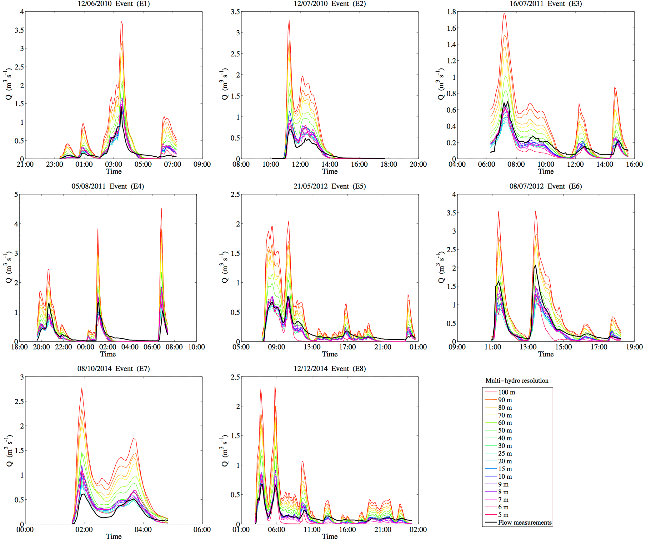
Figure 14Multi-scale modelling outputs compared with observed flow, showing the high sensitivity of Multi-Hydro response to the spatial resolution of the model.
5.2.1 Hydrodynamic evaluation
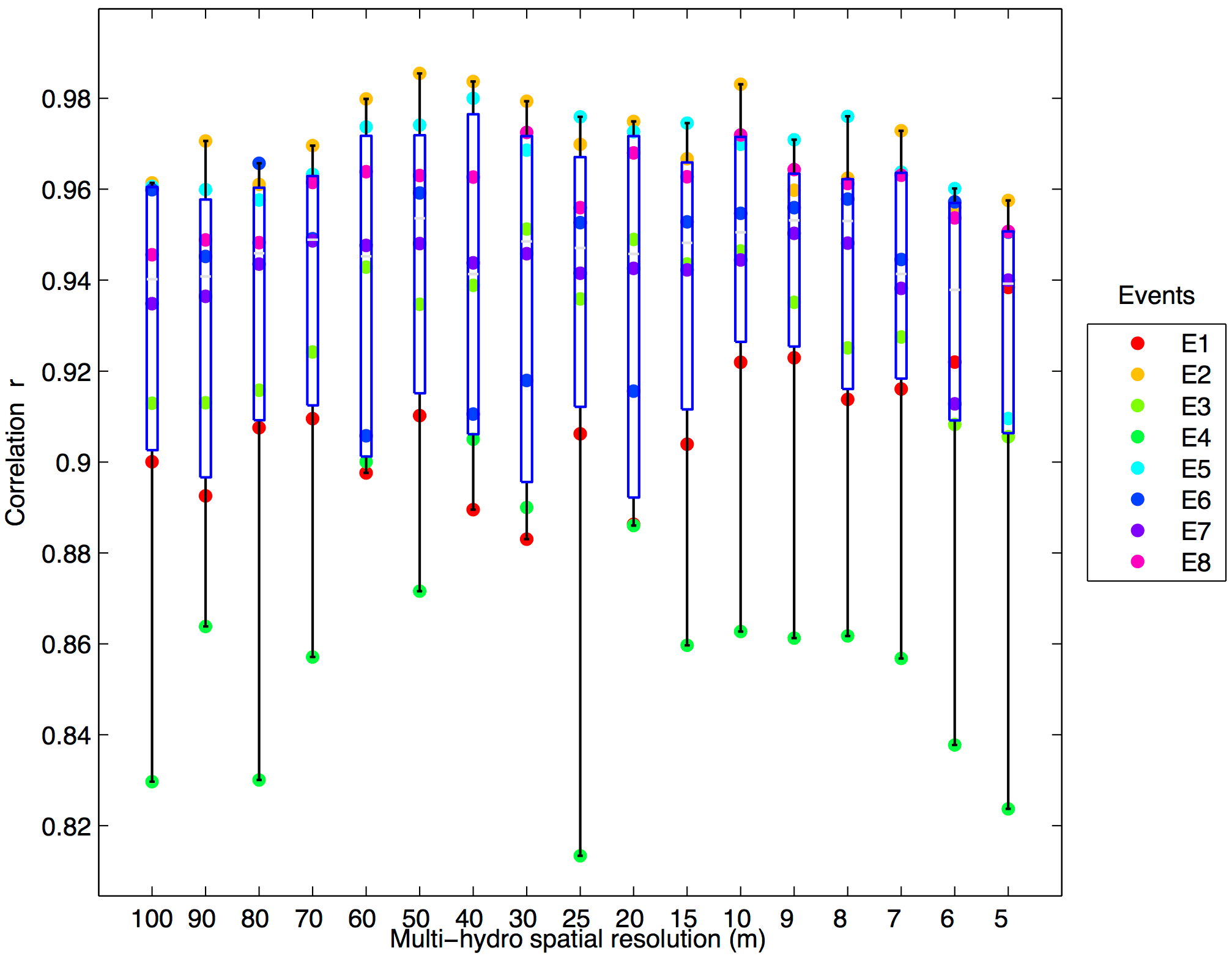
Figure 15Results of model hydrodynamic evaluation; the correlation coefficient r was retrieved for each modelling output with respect to real measurements.
The hydrodynamic evaluation aims to quantify the ability of the model to reproduce the flow dynamic observed in the measurements. It is based here on the estimation of the correlation coefficient r between modelled and observed data. The box plots are obtained from the computation of eight samples corresponding to the eight rainfall events. All the results obtained are plotted and no information was removed. The boxes corresponding to the 20 and 80 % quantiles were added only for indicative purpose. From Fig. 15, one can notice the high capacity of the Multi-Hydro model to reproduce the observed flow dynamic at any spatial scale. In fact, r values range between 0.85 and 0.98, with an average between 0.94 and 0.98, indicating high correlation between modelled and observed data. This trend was also noticed from visual inspection of modelling outputs and observed data (Fig. 14). This demonstrates the ability of this physically based model to reproduce correctly the observed flow dynamic, and also the rather good quality of the rainfall data, bearing in mind that the spatial variability is not taken into account. It also indicates that the physical parameters characterizing the behaviour of each land cover class, which were selected from their somewhat representative range and used for the implementation of the model, yield acceptable results whatever the chosen implementation scale. This suggests an alternative approach to the classical model calibration. Indeed, instead of tuning the parameters to force the model to reproduce the simulated flow, one can simply change the implementation scale to one enabling a proper representation of the catchment's land cover variability. As an illustration, the overestimation of the volume visible with coarse pixels is in fact mainly due to an overestimation of impervious areas observed with such pixel size. The next section will provide hints on how to select the appropriate modelling scale.
5.2.2 Performance evaluation
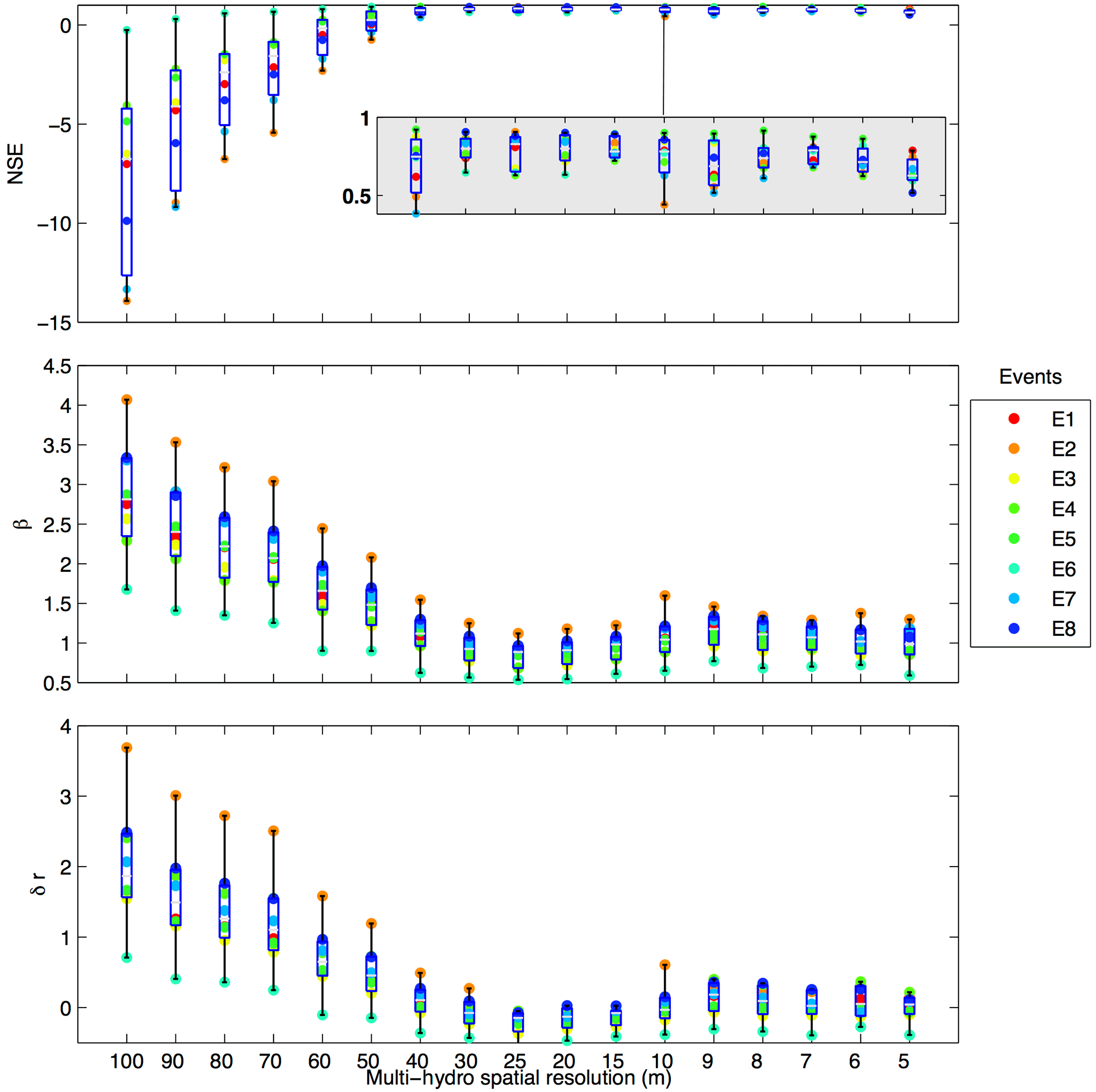
Figure 16Performance indicators NSE, β and δr estimated from Multi-Hydro modelling output obtained at the 17 spatial scales with respect to observed data.
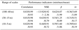
The multi-scale performance evaluation of Multi-Hydro model output is performed using the three statistical indicators presented in Sect. 4.2: NSE, the coefficient of regression β and the relative error at the peak flow δr. Obtained results are summarized in Fig. 16. Note the high scale dependence of the obtained model performance, which was not the case for the dynamic evaluation. In fact, all indicators reveal a similar trend of higher performance at small scales and lower performance at large scales. Model performance is indeed improved as the model resolution increases. From these results, the three ranges of scale previously identified with the help of the fractal analysis (Fig. 12) are also found in Fig. 16. Consequently, performance evaluation will be analysed at these three ranges of scale. Basic statistics (minimum, maximum and mean) of performance indicators Correlation, NSE, β and δr calculated for the three ranges of scales (100–40 m), (30–15 m) and (10–5 m) are displayed in Table 2.
Table 2Min/max/mean of performance indicators (Correlation, NSE, β and δr) calculated at three ranges of scale: (100–40 m), (30–15 m) and (10–5 m).
-
At large scales (100–40 m): the imperviousness coefficient Cimp of the catchment is very high, ranging from 45 % at 100 m to 30 % at 40 m. The modelled flow obtained at this range of scales exhibits similar dynamic as observed flow; however, performance indicators are bad. NSE values range from −13.92 observed at 100 m scale to 0.92 observed at 40 m scale. The β indicator suggests that the model is highly overestimating observed flow, with values ranging from 4.07 observed at 100 m scale to a minimum value of 0.62 noticed at 40 m, and an average around 2. This follows a trend similar to Cimp. In terms of the peak flow analysis, the relative error indicator (δr) shows clear overestimation of the peak flow at this range of scales, up to 369 %.
All statistic indicators suggest very weak performance of the model at large scales (100–40 m). In fact, the catchment behaviour at this range of scales is consistent with the high imperviousness coefficient observed, which means that infiltration is limited and water is in the majority of cases rapidly routed to the sewer system.
-
At medium scales (30–15 m): the model shows its best performance. NSE values range from 0.63 to 0.91, with an average around 0.79. The β indicator takes values between 0.54 and 1.25, and its mean is around 0.89, suggesting a good fit between modelled and observed data. The relative error indicator (δr) ranges from −0.31 to 0.51 with a mean value around 0.17, meaning that the model still overestimates the peak flow by 17 % on average.
-
At small scales (10–5 m): at this range of scales, the model performance remains high but potential trends with regards to scale are unclear. In fact, Table 2 indicates that NSE values range between 0.44 and 0.91 with a mean value around 0.72, demonstrating good performance of the Multi-Hydro model. The β indicator takes values between 0.59 and 1.6, with a mean around 1.06. The relative error indicator (δr) ranges from −0.39 to 0.61, with a mean value around 0.19. Slight fluctuations of the model performance are observed at this range of scales; the trend observed in statistics as a function of pixel size for large and medium scales (the improvement of all statistics as the pixel size decreases) is no longer valid at small scales, where fluctuations of statistics are noticed (they increase at 10 and 9 m before decreasing at 7 m). These fluctuations highlight some specific issues at this range of scales, which influence the model performance. This point will be discussed further in the next section.
5.2.3 Specific modelling issues at small scales
It is also important to discuss in this paper the performance of the model in a more global framework, especially by taking into consideration some serious problems that one may face when performing high-resolution modelling. In fact, as shown in Fig. 16, the model performance indeed increases with decreasing spatial scale of the model. This is due to a better representation of the catchment complexity, notably its scaling behaviour and the small-scale heterogeneity. However, three ranges of scales were clearly identified from previous results. At large scales (100–40 m), the model shows a fast computation time (up to only few minutes on a standard laptop) but lower performance (the model reproduces the same flow dynamic, but the volume is overestimated by up to 234 %). At medium scales (30–15 m), the model exhibits high performance (Table 2) and fast computation time. At small scales (10–5 m) the urban catchment configuration remains unchanged (the imperviousness coefficient remains around 37 %, compared to the medium scale); however, model performance at this range of scales is unclear and some fluctuations are noticed. Such fluctuations are in fact related to some non-trivial problems that only take place at small scales and should be considered when implementing urban storm models:
-
Quality of distributed data: urban hydrological models in general and fully distributed ones in particular are highly demanding with respect to the distributed data needed for their implementation. A detailed description of the land cover is essential as well as distributed topography data. Such data are usually available and can be provided by specialized services. However, quality is a big issue, especially when used to perform high-resolution modelling. Two main issues are highlighted here:
-
The spatial resolution of the topography data: the topography is the main driving force for surface water movements and the accuracy of these data has a lot of influence on grid-based models outputs. In our case, the topography data were available at 25 m resolution and interpolation was performed to obtain distributed data at small scales. However, the quality of obtained data below the 25 pixel grid is not fully reliable. The problem is even more striking for small scales down to 2 m (not included in this work, but details can be found in Ichiba, 2016), where the movements of water in the surface are very limited because the elevation gradient becomes very low.
-
Land cover description: the land cover is also of extreme importance in urban hydrology and specifically for fully distributed models. In fact, physical properties defined for each pixel depend exclusively on its land cover. Such data are usually available especially after huge improvements noticed in the availability of satellite images and new technologies used in this field. However, one commonly faced issue is the proportion of unknown data, indicating unidentified land cover. This is not related to the data resolution, but depends on the processing procedure of satellite and areal images obtained. In the case of Sucy-en-Brie catchment, land cover data were available at very good resolution (25 cm), but the proportion of unidentified data was about 20 % and was filled in most cases by grass. At large scales, the problem associated with “no data” pixels has limited influence, because large pixels usually include a large portion of well-identified land cover classes, like roads and houses. But at small scales, the catchment behaviour will be affected by the land cover attributed to these “no data” pixels, and the model response will not be the same if the unidentified areas are filled by grass or by impervious soil.
-
-
Numerical instabilities: fluctuation of the model performance noticed at small scales can also be the consequence of numerical instabilities. In fact, the numerical scheme used in the Multi-Hydro model for the surface modelling calculations is sensitive to small-scale variation, which affects the model response. Further works should be conducted to better quantify these instabilities.
-
Computation time: it is important in urban hydrology to consider the computation time needed for a model to simulate a given rainfall period. It is in fact one of the first criteria considered by urban water managers for the choice of urban storm models. Fast computation time is even crucial in the case of models used in real-time management processes. For fully distributed models, the computation time depends on two factors; the size of the catchment and the resolution of the model. For the case of Sucy-en-Brie catchment, the Multi-Hydro model shows fast computation time at large scales up to 10 m (a few minutes on a standard laptop), and huge computation time is needed at very small scales (5–2 m) (several hours). This is due to the numerical scheme, the modelling approach and the great number and size of the model outputs saved for research needs. Improvements should be implemented in the model structure in order to enhance the model performance from this point of view.
-
Mismatch between rainfall input resolution and model resolution: in this study, uniform rainfall input (rain gauge data) was applied to the catchment in all model simulations. Numerous authors have shown that model performance is strongly dependent on rainfall input resolution (Rafieeinasab et al., 2015; Ochoa-Rodriguez et al., 2015; Gires et al., 2015; Ichiba, 2016). Nevertheless, the aim of this study was to investigate the sensitivity of model performance to model resolution independently of rainfall resolution; therefore uniform rainfall was purposely input to the model. Future studies will look into the combined effects of rainfall and model resolution, based on the high-resolution rainfall data increasingly available.
-
Interactions between spatial and temporal resolution: In this study, a constant time resolution of 5 min was used for rainfall input, flow data and model simulations. Previous studies have shown that a dependence exists between spatial and temporal resolution of rainfall inputs and model simulation results (Rafieeinasab et al., 2015; Ochoa-Rodriguez et al., 2015; Gires et al., 2015; Ichiba, 2016). Both rainfall phenomena and hydrological processes exhibit scale dependence, both with respect to their spatial and temporal resolution. Previous studies have suggested that a fixed relationship could exist between spatial and temporal resolution and that the spatial resolution of rainfall input and model simulation cannot be changed independently of the temporal resolution. Future studies are planned to investigate this relationship and the implications it has for hydrological model simulations.
This work was motivated by the fact that on the one hand the inputs of the hydrological models exhibit scale-invariant features while on the other hand distributed models are implemented at a single resolution. Hence the question we tried to investigate in this paper is “at which resolution should we implement the model?” – bearing in mind practical constraints such as missing data at high resolution or longer computation time. The main goal of the paper is to investigate the existence and try to identify the appropriate resolution (or a range of resolutions) for Multi-Hydro implementation.
In the first part of the paper, fractal tools were used to characterize the scale dependence observed within distributed data (available in commonly used GIS formats) used to configure urban storm models. Both the structure of the sewer network and the distribution of impervious areas were analysed. Then multi-scale modelling investigations were carried out using the fully distributed model to analyse the effect of this scale dependence on the model performance.
The model was implemented at 17 spatial resolutions ranging from 100 to 5 m. The case study area is a 2.45 km2 urban catchment located southeast of Paris, in Val-de-Marne County.
Results coming from this work confirm the scale dependence of the obtained model outputs. In fact, model performance indeed increases with decreasing spatial scales. This is due to a better representation of the catchment small-scale heterogeneity and scaling behaviour, notably for the impervious areas which are immediately active during a rainfall event. At large scales (100–40 m), the model shows a fast computation time (only a few minutes) and also reproduces well the overall flow dynamic, but the flow volumes remain largely overestimated. At small scales (10–5 m) the urban catchment configuration, including the overall imperviousness, becomes scale independent, without any further improvement, and one can notice a possible decline of the model performance. The small fluctuations of the model performance at this range of scales are in fact related to specific issues taking place at high resolution: mainly data problems, such as GIS data quality and missing information, as well as model numerical instabilities, without ignoring the computation time constraints essential for urban hydrology applications.
Over the remaining medium range of scales (30–15 m) for our case study, the model exhibits high performance and fast computation time since the increase in data resolution creates sufficient spatial variability among the grid-based parameters of the model. Such variability becomes somewhat representative (i.e. up to the selected precision) for the geophysical variability of the studied urban catchment.
Due to a tremendous increase in number of data pixels for grid-based models, one easily understands the difficulty of applying the classical methods for model parameter calibration. Analysis performed here demonstrates that forcing the model to give a better performance by changing its parameters is simply not reasonable for grid-based models because of their strong scale dependence. In turn, such scaling dependence induces an alternative to the classical model calibration. As we have demonstrated here, a better consideration of such scale dependence makes it possible to define an optimum range of scales – over which the model performs much better with respect to the measurements. This can be seen as a proposed alternative to the classical parameter calibration of grid-based models.
GIS data as well as all rainfall and flow measurements were made available by the CG94 as part of a collaboration agreement that prevents the publication of these data. The Multi-Hydro model is available upon request from the HMCo Lab (http://hmco.enpc.fr).
The authors declare that they have no conflict of interest.
The authors acknowledge both the European project INTERREG RainGain
(http://www.raingain.eu) and the ANRT association
(http://www.anrt.asso.fr) for their financial support of this work. The
first author thanks the DSEA94 (Direction des Services de
l'Environnement et de l'Assainissement) for providing data sets used in this
work. A partial financial support of the Chair “Hydrology for resilient
cities” endowed by Veolia is gratefully acknowledged.
Edited by: Nadia Ursino
Reviewed by: Jamal
Alikhani and one anonymous referee
Blöschl, G. and Sivapalan, M.: Scale issues in hydrological modelling: A review, Hydrol. Process., 9, 251–290, 1995. a, b
Daniel, E. B., Camp, J. V., LeBoeuf, E. J., Penrod, J. R., Dobbins, J. P., and Abkowitz, M. D.: Watershed modeling and its applications: A state-of-the-art review, Open Hydrology Journal, 5, 26–50, 2011. a
Dehotin, J. and Braud, I.: Which spatial discretization for distributed hydrological models? Proposition of a methodology and illustration for medium to large-scale catchments, Hydrol. Earth Syst. Sci., 12, 769–796, https://doi.org/10.5194/hess-12-769-2008, 2008. a, b
El Tabach, E., Tchiguirinskaia, I., and Mahmood, O., and Schertzer: Multi-Hydro: a spatially distributed numerical model to assess and manage runoff processes in peri- urban watersheds, in: Proceedings Final conference of the COST Action C22 Urban Flood Management, Paris, France, 26 November 2009. a
Elliott, A. H. and Trowsdale, S. A.: A review of models for low impact urban stormwater drainage, Environ. Modell. Softw., 22, 394–405, 2007. a
Elliott, A. H., Trowsdale, S. A., and Wadhwa, S.: Effect of Aggregation of On-Site Storm-Water Control Devices in an Urban Catchment Model, J. Hydrol. Eng., 14, 975–983, 2009. a
England, Jr., J. F., Velleux, M. L., and Julien, P. Y.: Two-dimensional simulations of extreme floods on a large watershed, J. Hydrol., 347, 229–241, 2007. a
Frankhauser, P.: The Fractal Approach. A New Tool for the Spatial Analysis of Urban Agglomerations, Population: An English Selection, 10, 205–240, 1998. a
Ghosh, I. and Hellweger, F. L.: Effects of Spatial Resolution in Urban Hydrologic Simulations, J. Hydrol. Eng., 17, 129–137, 2012. a
Giangola-Murzyn, A.: Modélisation et paramétrisation hydrologique de la ville, résilience aux inondations, PhD thesis, Université Paris-Est, 2013. a, b, c, d
Gires, A., Onof, C., Maksimovic, C., Schertzer, D., Tchiguirinskaia, I., and Simoes, N.: Quantifying the impact of small scale unmeasured rainfall variability on urban runoff through multifractal downscaling: A case study, J. Hydrol., 442–443, 117–128, 2012. a
Gires, A., Tchiguirinskaia, I., Schertzer, D., and Lovejoy, S.: Multifractal analysis of a semi-distributed urban hydrological model, Urban Water J., 10, 195–208, 2013. a, b
Gires, A., Giangola-Murzyn, A., Abbes, J.-B., Tchiguirinskaia, I., Schertzer, D., and Lovejoy, S.: Impacts of small scale rainfall variability in urban areas: a case study with 1D and 1D/2D hydrological models in a multifractal framework, Urban Water J., 12, 607–617, 2014. a, b
Gires, A., Giangola-Murzyn, A., Abbes, J.-B., Tchiguirinskaia, I., Schertzer, D., and Lovejoy, S.: Impacts of small scale rainfall variability in urban areas: a case study with 1D and 1D/2D hydrological models in a multifractal framework, Urban Water J., 12, 607–617, 2015. a, b
Gires, A., Tchiguirinskaia, I., Schertzer, D., Ochoa-Rodriguez, S., Willems, P., Ichiba, A., Wang, L.-P., Pina, R., Van Assel, J., Bruni, G., Murla Tuyls, D., and ten Veldhuis, M.-C.: Fractal analysis of urban catchments and their representation in semi-distributed models: imperviousness and sewer system, Hydrol. Earth Syst. Sci., 21, 2361–2375, https://doi.org/10.5194/hess-21-2361-2017, 2017. a, b, c
Goldberger, A. L. and West, B. J.: Fractals in physiology and medicine, Yale J. Biol. Med., 60, 421–435, 1987. a
Gupta, H. V., Kling, H., Yilmaz, K. K., and Martinez, G. F.: Decomposition of the mean squared error and NSE performance criteria: Implications for improving hydrological modelling, J. Hydrol., 377, 80–91, 2009. a
Healy, R. W.: Simulation of solute transport in variably saturated porous media with supplemental information on modifications to the US Geological Survey's computer program VS2D, Department of the Interior, US Geological Survey, 1990. a
Hromadka II, T. V.: The state-of-the-art in hydrologic models, Environ. Softw., 2, 29–36, https://doi.org/10.1016/0266-9838(87)90026-8, 1987. a
Ichiba, A.: X-band radar data and predictive management in urban hydrology, Ph.D. thesis, Universite Paris-Est, 2016. a, b, c, d, e, f, g, h, i, j
Insa-Valor, S.: Canoe: logiciel d'hydrologie urbaine, conception et evaluation de reseaux d'assainissement, simulation des pluies, des ecoulements et de la qualite des eaux, Manuel de l'utilisateur, 1999. a
James, W., Rossman, L. A., and James, W. R. C.: User's guide to SWMM 5:[based on original USEPA SWMM documentation], 2010. a
Jiang, S., Shiguo, J., and Desheng, L.: Box-Counting Dimension of Fractal Urban Form, International Journal of Artificial Life Research, 3, 41–63, 2012. a
Kleidorfer, M., Deletic, A., Fletcher, T. D., and Rauch, W.: Impact of input data uncertainties on urban stormwater model parameters, Water Sci. Technol., 60, 1545–1554, https://doi.org/10.2166/wst.2009.493, 2009. a
Lappala, E. G., Healy, R. W., and Weeks, E. P.: Documentation of computer program VS2D to solve the equations of fluid flow in variably saturated porous media, Department of the Interior, US Geological Survey, 1987. a, b
Lovejoy, S. and Schertzer, D.: Multifractals, universality classes and satellite and radar measurements of cloud and rain fields, J. Geophys. Res., 95, 2021–2034, 1990. a
Mandelbrot, B. B.: The fractal geometry of nature, vol. 173, Macmillan, 1983. a
Mesev, T. V., Longley, P. A., Batty, M., and Xie, Y.: Morphology from Imagery: Detecting and Measuring the Density of Urban Land Use, Environ. Plann. A, 27, 759–780, 1995. a
Multi-Hydro: Official number: IDDN.FR.001.340017.000.S.C.2015.
0000.31235,
Agence de Protection des Programmes (French Agency for software protection),
2015. a
Niu, H., Wang, J., and Lu, Y.: Fluctuation behaviors of financial return volatility duration, Physica A, 448, 30–40, 2016. a
Nonnenmacher, T. F., Losa, G. A., and Weibel, E. R.: Fractals in Biology and Medicine, Birkhäuser, Basel, 2013. a
Ochoa-Rodriguez, S., Wang, L.-P., Gires, A., Pina, R. D., Reinoso-Rondinel, R., Bruni, G., Ichiba, A., Gaitan, S., Cristiano, E., van Assel, J., Kroll, S., Murlà-Tuyls, D., Tisserand, B., Schertzer, D., Tchiguirinskaia, I., Onof, C., Willems, P., and ten Veldhuis, M.-C.: Impact of spatial and temporal resolution of rainfall inputs on urban hydrodynamic modelling outputs: A multi-catchment investigation, J. Hydrol., 531, 389–407, https://doi.org/.10.1016/j.jhydrol.2015.05.035, 2015. a, b
Ostrowski, M. W.: Modeling urban hydrological processes and management scenarios at different temporal and spatial scales, Best Modeling Practices for Urban Water Systems, Monograph, 10, 27–40, 2002. a
Park, S. Y., Lee, K. W., Park, I. H., and Ha, S. R.: Effect of the aggregation level of surface runoff fields and sewer network for a SWMM simulation, Desalination, 226, 328–337, 2008. a, b
Radziejewski, M. and Kundzewicz, Z. W.: Fractal analysis of flow of the river Warta, J. Hydrol., 200, 280–294, 1997. a
Rafieeinasab, A., Norouzi, A., Kim, S., Habibi, H., Nazari, B., Seo, D.-J., Lee, H., Cosgrove, B., and Cui, Z.: Toward high-resolution flash flood prediction in large urban areas – Analysis of sensitivity to spatiotemporal resolution of rainfall input and hydrologic modeling, Journal of Hydrology, 531, Part 2, 370–388, https://doi.org/10.1016/j.jhydrol.2015.08.045, 2015. a, b
Refsgaard, J. C. and Knudsen, J.: Operational Validation and Intercomparison of Different Types of Hydrological Models, Water Resour. Res., 32, 2189–2202, 1996. a
Sagar, B. S. D.: Fractal dimension of non-network space of a catchment basin, Geophys. Res. Lett., 31, L12502, https://doi.org/10.1029/2004GL019749, 2004. a
Salvadore, E., Bronders, J., and Batelaan, O.: Hydrological modelling of urbanized catchments: A review and future directions, Part 1, J. Hydrol., 529, 62–81, 2015. a, b
Sarma, P. B. S., Delleur, J. W., and Rao, A. R.: Comparison of rainfall-runoff models for urban areas, J. Hydrol., 18, 329–347, 1973. a
Schertzer, D. and Lovejoy, S.: Physical modeling and analysis of rain and clouds by anisotropic scaling multiplicative processes, J. Geophys. Res.-Atmos., 92, 9693–9714, 1987. a
Stephenson, D.: Selection of Stormwater Model Parameters, J. Environ. Eng., 115, 210–220, 1989. a, b
Tech University of Darmstadt and Ostrowski, M.: Modeling Urban Hydrological Processes and Management Scenarios at Different Temporal and Spatial Scales, JWMM, 2002. a
Thibault, S. and Crews, J.: The morphology and growth of urban technical networks: a fractal approach, flux, 19, 17–30, 1995. a
Turcotte, D. L.: Fractals in Geology and Geophysics, in: Fractals in Geophysics, edited by: Scholz, C. H. and Mandelbrot, B. B., Pure and Applied Geophysics, Birkhäuser, Basel, 171–176, 1989. a
Turcotte, D. L. and Huang, J.: Fractal Distributions in Geology, Scale Invariance, and Deterministic Chaos, in: Fractals in the Earth Sciences, edited by: Barton, C. C. and La Pointe, P. R., 1–40, Springer US, 1995. a
Velleux, M. L., England, Jr., J. F., and Julien, P. Y.: TREX: spatially distributed model to assess watershed contaminant transport and fate, Sci. Total Environ., 404, 113–128, 2008. a, b
Versini, P.-A., Gires, A., Tchinguirinskaia, I., and Schertzer, D.: Toward an operational tool to simulate green roof hydrological impact at the basin scale: a new version of the distributed rainfall–runoff model Multi-Hydro, Water Sci. Technol., 74, 1845–1854, 2016. a, b
West, B. J.: Fractal Physiology and Chaos in Medicine, World Scientific, 2012. a
Wood, E. F., Sivapalan, M., Beven, K., and Band, L.: Effects of spatial variability and scale with implications to hydrologic modeling, J. Hydrol., 102, 29–47, 1988. a, b
Wu, H., Sun, Y., Shi, W., Chen, X., and Fu, D.: Examining the Satellite-Detected Urban Land Use Spatial Patterns Using Multidimensional Fractal Dimension Indices, Remote Sens., 5, 5152–5172, 2013. a
Wu, J. and He, C.: Experimental and modeling investigation of sewage solids sedimentation based on particle size distribution and fractal dimension, Int. J. Environ. Sci. Technol., 7, 37–46, 2009. a
Yanshi, X. and Kaixuan, T.: Fractal research on fracture structures and application in geology, Geology-Geochemistry, 30, 71–77, 2002. a
Zhang, W. and Montgomery, D. R.: Digital elevation model grid size, landscape representation, and hydrologic simulations, Water Resour. Res., 30, 1019–1028, 1994. a, b