the Creative Commons Attribution 4.0 License.
the Creative Commons Attribution 4.0 License.
 | 13 Jun 2018
On the appropriate definition of soil profile configuration and initial conditions for land surface–hydrology models in cold regions
Gonzalo Sapriza-Azuri
Pablo Gamazo
Saman Razavi
Howard S. Wheater
Arctic and subarctic regions are amongst the most susceptible regions on Earth to global warming and climate change. Understanding and predicting the impact of climate change in these regions require a proper process representation of the interactions between climate, carbon cycle, and hydrology in Earth system models. This study focuses on land surface models (LSMs) that represent the lower boundary condition of general circulation models (GCMs) and regional climate models (RCMs), which simulate climate change evolution at the global and regional scales, respectively. LSMs typically utilize a standard soil configuration with a depth of no more than 4 m, whereas for cold, permafrost regions, field experiments show that attention to deep soil profiles is needed to understand and close the water and energy balances, which are tightly coupled through the phase change. To address this gap, we design and run a series of model experiments with a one-dimensional LSM, called CLASS (Canadian Land Surface Scheme), as embedded in the MESH (Modélisation Environmentale Communautaire – Surface and Hydrology) modelling system, to (1) characterize the effect of soil profile depth under different climate conditions and in the presence of parameter uncertainty; (2) assess the effect of including or excluding the geothermal flux in the LSM at the bottom of the soil column; and (3) develop a methodology for temperature profile initialization in permafrost regions, where the system has an extended memory, by the use of paleo-records and bootstrapping. Our study area is in Norman Wells, Northwest Territories of Canada, where measurements of soil temperature profiles and historical reconstructed climate data are available. Our results demonstrate a dominant role for parameter uncertainty, that is often neglected in LSMs. Considering such high sensitivity to parameter values and dependency on the climate condition, we show that a minimum depth of 20 m is essential to adequately represent the temperature dynamics. We further show that our proposed initialization procedure is effective and robust to uncertainty in paleo-climate reconstructions and that more than 300 years of reconstructed climate time series are needed for proper model initialization.
- Article
(4484 KB) - Full-text XML
- BibTeX
- EndNote


Arctic and subarctic regions are amongst the most susceptible on Earth to climate change (IPCC, 2013; Hinzman et al., 2005). For example, shrub expansion into the tundra regions (Sturm et al., 2001), permafrost thaw (Connon et al., 2014; Rowland et al., 2010), and glacier retreat (Marshall, 2014) are some of the current manifestations of climate change. All these changes are triggered by the interaction of climate, the carbon cycle, and hydrology in response to global warming (Schuur et al., 2015). These effects are expected to be exacerbated due to global warming trends in the coming years (IPCC, 2013; Slater and Lawrence, 2013; Lawrence and Slater, 2005). Therefore, being able to evaluate and assess the impact of climate change in cold regions is a primary concern for the scientific community, stakeholders, and First Nations communities in northern regions. The significance of this problem in Canada has led to the creation of the Changing Cold Regions Network (DeBeer et al., 2015; http://www.ccrnetwork.ca, last access: 5 September 2017), which aims to provide improved science and modelling to address these concerns.
Earth system models are essential tools for evaluating the impacts of climate change. At global and regional scales, general circulation models (GCMs) and regional climate models (RCMs) are used to simulate climate change evolution. Land surface models (LSMs) are used with GCMs and RCMs (coupled or offline) to represent the hydrological processes associated with the lower boundary condition of the atmosphere. These models typically represent the coupled energy and water balance in the soil, based on numerical solution of the Richards equation and using a relatively coarse vertical discretization.
In general, a standard soil configuration with a depth of no more than 4 m is used in all LSMs that are commonly implemented in GCMs and RCMs (see for example the comparison made by Slater and Lawrence, 2013, for the soil configuration depth (SCD) in LSMs implemented in some GCMs). The typical boundary conditions to solve the energy and water balance in the soil column are (1) the exchanges with atmosphere at the top, (2) no lateral exchange of water or energy with the surrounding grids (only vertical fluxes), and (3) no heat flux at the bottom of the soil.
For moderate climate conditions and at the spatial scales on which these models are commonly applied, the above depth and boundary conditions are commonly deemed to be sufficient to capture the intra-annual variability in the energy and water balance. However, for cold regions, where the energy balance is closely related to the water balance through the phase change (Woo, 2012), deeper soil configurations and more representative boundary conditions are needed. A deeper soil profile in a model can result in a more accurate process representation as it allows the heat signal to propagate to deeper soil layers and hence avoids erroneous near-surface states and fluxes, such as overheating or over-freezing during summer and winter, respectively (e.g, Lawrence et al., 2008; Stevens et al., 2007). An alternative to modelling a deeper soil profile is the incorporation of a rigorous lower boundary condition that adaptively changes with time and includes a geothermal heat flux (Hayashi et al., 2007). Developing and incorporating a dynamic lower boundary condition is, however, impractical in most cases due to lack of adequate data; in addition, the geothermal heat flux is usually ignored in LSMs, as its effects on temperature dynamics within the upper 20–30 m of soil are considered negligible on century timescales (Nicolsky et al., 2007).
The aforementioned challenges and shortcomings have been recognized by the climate, permafrost, and hydrology community. For climate models, Slater and Lawrence (2013), Alexeev et al. (2007), Nicolsky et al. (2007), and Stevens et al. (2007) have disputed the validity of GCM future projections due to the shallow soil profile depth in LSMs for the reasons stated above. There have been studies of how the spatial distribution of permafrost is improved by including deeper soil configurations in an LSM. For example, Paquin and Sushama (2015) considered a 65 m deep soil configuration for the arctic region with a spin-up period of 200 years through recycling the 1970–1999 period in the Canadian RCM, which uses Canadian Land Surface Scheme (CLASS) (Verseghy, 1991) as the LSM, and showed an improved spatial distribution of permafrost. Zhang et al. (2003, 2006, 2008) used a thermal soil model that includes soil water balance and showed the importance of considering deep soil configurations. In the context of LSMs, Troy et al. (2012) simulated river basins in northern Eurasia using a 50 m soil configuration with a spin-up of 500 years by recycling the 1901–2001 period 5 times. Decharme et al. (2013), who applied the ISBA model to the whole of France, concluded that an 18 m depth was needed to properly simulate the energy and water balance.
In addition, deeper soil/rock configurations possess extended system memories, and, as such, particular care should be taken to properly define the initial conditions for the subsurface system. The presence of significant non-stationarity in climate and hydrology further complicates the process of model initialization, as it leads to significant changes to the statistical properties and envelope of variability of forcings (Razavi et al., 2015). Due to such non-stationarity, it may be inadvisable to initialize a model by recycling the (typically short) historical records (i.e., repeating the simulation over the same period multiple times and using the final model state of one run as the initial state of the next run), as implemented in Troy et al. (2012) or Paquin and Sushama (2015); such practice, in particular, may result in serious misrepresentation of soil processes, because the significant warming trend in the historical records of cold regions leads to unrealistically warmer soil states after each cycle. Together, these reasons highlight the pressing need for multi-century-long hydroclimatic records to include past non-stationarity that may affect the present state and flux variables. Proxy records such as tree rings can provide a vehicle to reconstruct long hydroclimatic time series, typically at annual to multi-year timescales (Razavi et al., 2016).
The sensitivity of LSMs to initial conditions and the initialization methods has been the focus of several studies (e.g., Yang et al., 1995; Rodell et al., 2005; Shrestha and Houser, 2010). However, most of these works have focused on relatively shallow soil profiles located in areas other than cold regions. An exception is the work of Ednie et al. (2008) that illustrated the need for a suitable model initialization procedure to properly simulate soil thermal profiles in permafrost regions and applied a simplified thermal model of soil by using reconstructed past climate variables.
Despite significant advances, as briefly outlined above, the appropriate soil configuration depth in land surface modelling of cold regions remains an open question. This question is further complicated by the fact that parameter uncertainty is typically ignored in LSMs, and parameter values are usually collected from look-up tables based on land cover and soil maps (Mendoza et al., 2015). Related to this, there have been some previous efforts for “sensitivity analysis” of model outputs to parameters (Razavi and Gupta, 2015) but these have been mainly limited to comparisons of different cover types (e.g., Paquin and Sushama, 2015; Yang et al., 1995) with some few exceptions (e.g., Bastidas et al., 2006).
In this paper, we focus on the three interrelated aspects of LSMs, namely soil depth, parameter uncertainty, and initializations, together to address the above question. Unlike the previous studies that focus on each aspect in isolation, this study looks at their joint and individual effects. We set up a series of systematic modelling experiments with the following three objectives to (1) identify the appropriate SCD for a given LSM and location in the presence of uncertainty in model parameter values and climate conditions, (2) assess the significance of including or excluding geothermal flux as the lower boundary condition in an LSM, and (3) develop an initialization procedure for LSMs in cold regions based on paleo-reconstructions of climate variables and statistical bootstrapping.
To advance our understanding and modelling capability of soil moisture and energy dynamics in permafrost regions, we developed two series of numerical experiments for a study area located in the Northwest Territories, Canada, where observations of soil temperature at several depths and historical reconstructed climate data are available.
2.1 Study area and data
The experimental test case is located at Norman Wells, in the Mackenzie Valley, Northwest Territories, Canada (Fig. 1). Based on the Permafrost Map of Canada (Geological Survey of Canada, 2000), the area is located in a zone of extensive discontinuous permafrost. The land cover is characterized by moss lichen groundcover, ericaceous shrubs, and black spruce and tamarack trees (Smith et al., 2004). The subsurface is formed by ice-rich silt clays. The climate of the region is subarctic, according to the Köppen climate classification (Peel et al., 2007), with an average annual mean daily temperature of −5 ∘C and average annual precipitation of 295 mm yr−1.
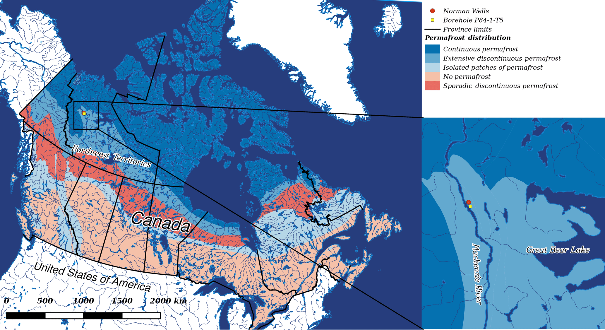
Figure 1Permafrost Map of Canada and location of the area of study. Temperature soil profiles are available at the borehole P84-1-T5 (yellow dot).
This area is selected due to the availability of both soil temperature at several depths down to 20 m (Smith et al., 2004) and dendroclimatic reconstructions of summer air temperature (Szeicz and MacDonald, 1995). These data will be used to test the proposed methodology to define the SCD and the initialization approach.
2.1.1 Soil temperature profiles
Annual soil temperature profiles are available based on the maximum and minimum daily average of soil temperature at several borehole locations in the Mackenzie Valley, administrated by the Geological Survey of Canada (Smith et al., 2004). Figure 2 shows the temperature profiles for the borehole 84-1-T5 selected for our analysis. The soil temperatures were measured at the following depths (in metres) for the period 1985–2001: . The active layer thickness, defined as the soil depth that encapsulates the seasonal freeze-and-thaw cycle (Woo, 2012), was also reported and varied from 1.5 m at the beginning of the period of record (1985) up to 3.0 m to the end of the period (2000), showing an increasing trend in the active layer thickness over time.
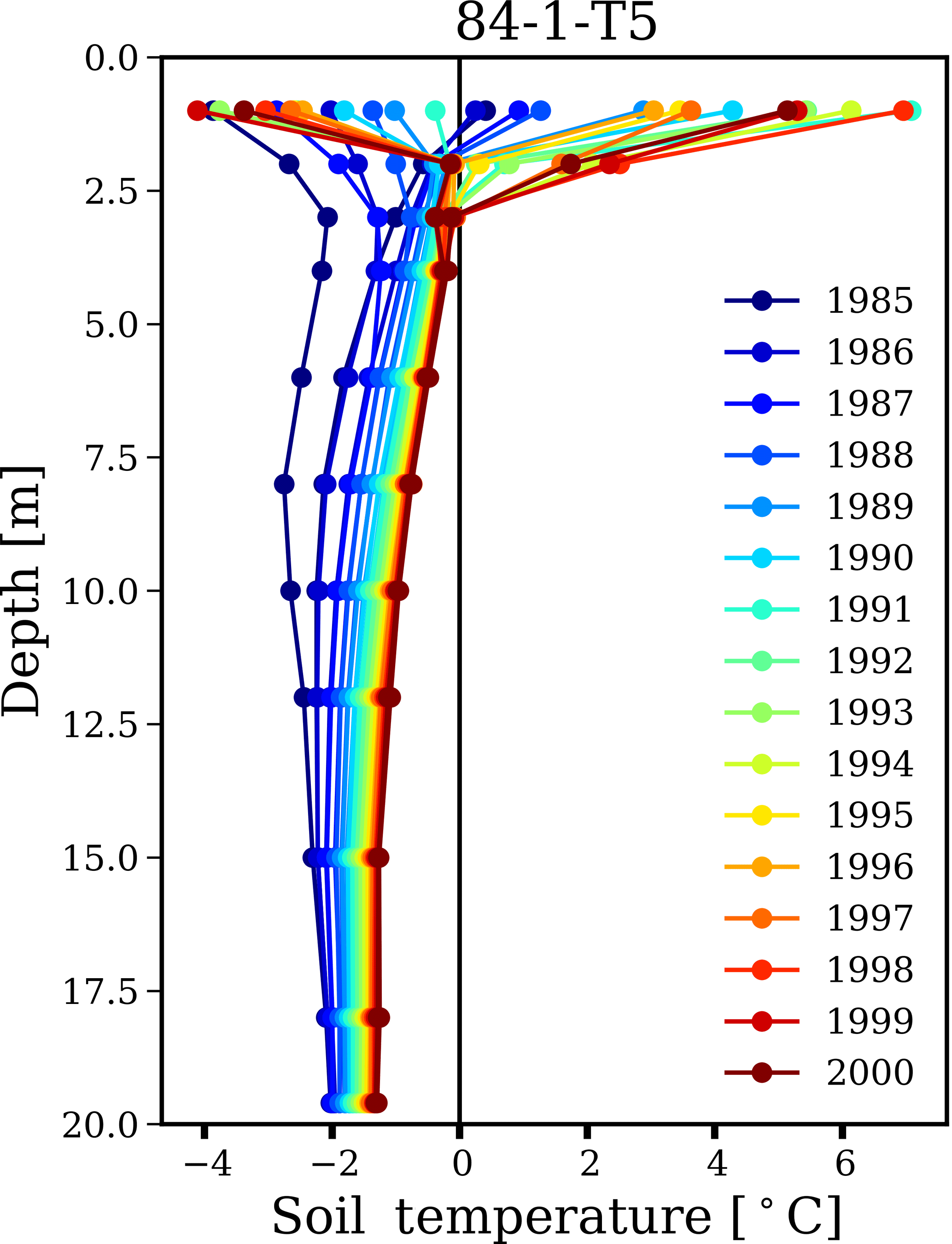
Figure 2Permafrost Annual maximum and minimum soil temperature profiles for the borehole 84-1-T5 located in Normal Wells. Each colour represent an individual year (1985–2000).
2.1.2 Reconstructed summer air temperature
Szeicz and MacDonald (1995) generated proxy climate records of average summer (June–July) air temperature based on tree rings for the period 1638–1988 in northwestern Canada near to Norman Wells (Fig. 3). These proxy data have been previously used by other authors (Ednie et al., 2008; Esper et al., 2002). For example, Ednie et al. (2008) showed that the linear trend of proxy summer air temperature can be used as an approximation of the linear trend of the mean annual air temperature for the region. Following this approach, we generate a stochastic climate time series (Sect. 2.5.1) that follows the historical reconstructions of mean annual air temperature based on the proxy data of Szeicz and MacDonald (1995).
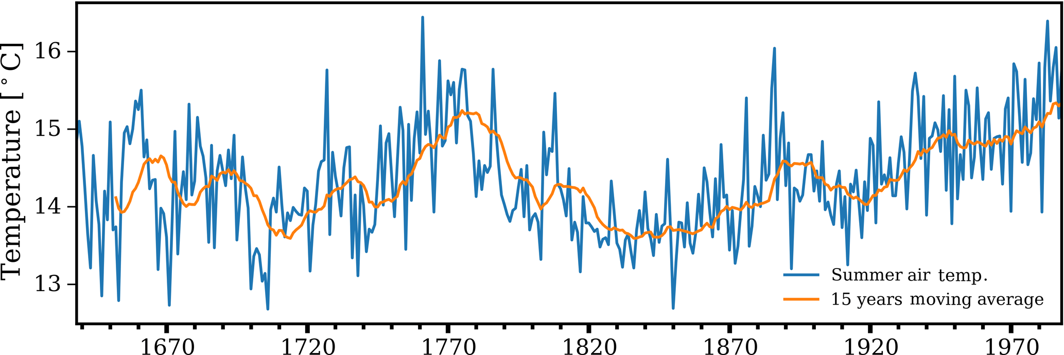
Figure 3Reconstructed summer (June–July) air temperature based on tree rings for the period 1638–1988 along with its 15-year moving average.
2.2 Design of experiments
The methodology and experiments were designed to be carried out in two stages. In the first stage, we focus on the characterization of the adequate soil profile depth for land surface–hydrologic modelling in the permafrost regions, in relation to climate condition and model parameterization. For this purpose, we run a 1-D model under a variety of soil profile, parameter, climate configurations, and lower boundary conditions. This stage is referred to as “Experiment 1” in this paper.
In the second stage, “Experiment 2”, we propose a method to handle the presence of non-stationarity in climate and hydrology, in order to include effects of past non-stationarity on the present state and flux variables. This method utilizes paleo-climate reconstructions to generate long, synthetic time series of climate variables for model initialization.
2.3 The 1-D model
The core of the experiments is a 1-D model implemented in MESH, Environment and Climate Change Canada's community model (Pietronero et al., 2007). This integrates the CLASS LSM (Verseghy et al., 1993; Verseghy, 1991), which solves coupled energy and water balance equations for vegetation, snow and soil and their exchange of heat and moisture with the atmosphere, and WATROF (Soulis et al., 2000) or PDMROF (Mekonnen et al., 2014) to solve the horizontal flow processes for basin-scale integration. MESH discretizes the spatial domain based on regular grid cells and each individual cell is then subdivided in grouped response units (GRUs) based on land cover and/or soil types. MESH has been commonly used to simulate land surface–hydrology processes in many cold regions (e.g., Yassin et al., 2017; Haghnegahdar et al., 2017). The 1-D CLASS model is implemented here at one grid cell, and a unique GRU was used. The upper boundary condition of the model is formed by atmospheric forcings. At the lower boundary condition, in terms of heat, we include two cases: no heat flux and geothermal flux (only in Experiment 1) and, in terms of mass, we assume the water flux that reaches the bottom of the soil profile drains to generate base flow. The climate forcings needed are temperature, precipitation, shortwave radiation, longwave radiation, specific humidity, wind velocity, and atmospheric pressure.
2.4 Experiment 1
A schematic representation of the modelling experiment is illustrated in Fig. 4. Several 1-D model set-ups were implemented by a combination of (1) various SCDs, (2) several climate conditions selected to spin up the model, (3) different values for the parameters that control hydrological processes (water and energy balance), and (4) the inclusion or exclusion of the geothermal flux as the lower boundary condition.
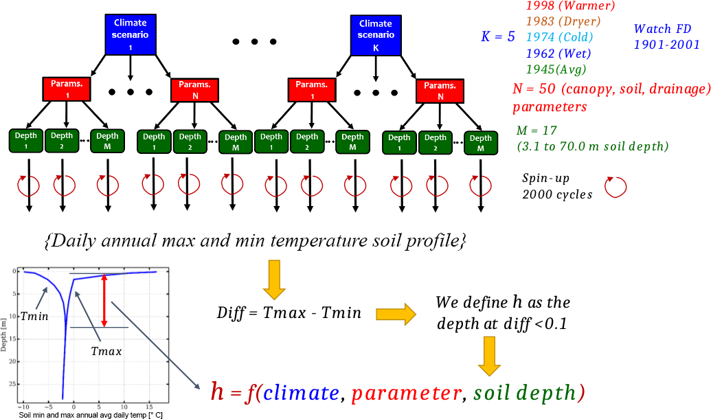
Figure 4Schematic representation of the model experiment for Experiment 1. The model set-ups are defined as combinations of 5 different climate conditions, 50 randomly selected sets of parameter values within their uncertainty ranges, and 17 different soil configurations. Each model is then run in a spin-up mode for 2000 cycles. The last year of spin-up is taken to compute the daily annual maximum and minimum soil temperature profiles and their difference is computed. The depth at which this difference becomes less than 0.1 is referred to as the “non-oscillation depth” or hT-non-oscillation.
2.4.1 Variable soil depth configuration
For this experiment, a series of 1-D models with incremental numbers of soil layers (corresponding to different total soil depths) are defined. The soil configurations of the 1-D models are illustrated in Fig. 5, as well as the range from the standard CLASS configuration of three layers with a 4.1 m depth to 20 layers corresponding to a depth of 71.59 m. The thickness of each layer is increased exponentially for deeper soil layers. A total of 17 different soil configurations are tested.

Figure 5The variable soil configuration profiles defined for the 1-D model: number of soil layers, depth of each layer, and total depth. Each colour represents a group of layers that are assigned the same parameter values. Panel (a) shows all the configurations and panel (b) shows a zoom-in window of the previous panel for the first few layers. The first soil configuration (three layers) represents the standard CLASS soil model configuration.
2.4.2 Climate conditions
To account for the effect of climate conditions, years 1998 (warm), 1983 (dry), 1974 (cold), 1962 (wet), and 1945 (average) (Table 1) are used with every model configuration. Each model was run five times (for the 5 years) over 2000-year-long sequences, each of which comprised 2000 back-to-back repetitions of 1 of the above years. These five climate conditions are defined based on temperature and precipitation obtained from the WATCH FD (WCH-FD) gridded data base of climate forcing (Weedon et al., 2011) for the period 1901–2001 at the location of our study area. We do not use the historical sequence of years 1901–2001 to avoid overheating effects that could be introduced due to the warming trend of the last century.
2.4.3 Parameter uncertainty
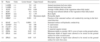
Three groups of parameters representing canopy, soil, and drainage processes are perturbed within their ranges of uncertainty to analyze their influence on SCD. Table 2 describes all the parameters considered along with their lower and upper bounds of variation. Monte Carlo sampling with a uniform distribution is applied to generate a collection of 50 samples for each parameter. The range of the canopy parameter values used represents different vegetation covers that are present in the area based on the look-up table from the CLASS user manual (Versegey, 2009). To set a consistent parametrization scheme for the soil texture across the models with different numbers of layers, we grouped layers and assigned the same values to the parameters of the layers in each group. These groups are represented with different colours in Fig. 5.
Table 1Climate conditions of the 5 representative years used in this study.
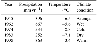
Table 2List, description, and ranges of model parameters perturbed in this study. The values of soil texture parameters SAND, CLAY, and ORG (denoted by *) sampled such that they sum to 100 %.
2.4.4 Lower boundary conditions: the geothermal flux
To assess the effect of the lower boundary condition on the energy balance and soil temperature profile, an analysis was made to compare two scenarios: (1) no heat flow at the bottom of the lowest soil layer and (2) a constant geothermal flow (called ggeo flux in CLASS). The comparative analysis was carried out for the average climatic condition (year 1945). All the 17 different soil configurations and 50 sets of parameter values were tested, resulting in a total of 850 model configurations to be run for scenario 2 above. For this scenario, the geothermal heat flow was set to be 0.083 W m−2, based on measurements made in a borehole in Norman Wells (Garland and Lennox, 1962).
2.4.5 Non-oscillation depth
In Experiment 1, we ran a total of = 5100 model combinations. In each of these model set-ups, a 2000-year model run was performed. All the models were set with the same initial conditions and constant temperature and liquid/ice saturation soil profiles. The soil thermal profile was defined at −3.0 ∘C and all the soil water was defined as ice content. We assume that after the spin-up a quasi-equilibrium between the climate conditions and the ground thermal state was reached. The last cycle, a complete 1-year simulation, was used to compute the annual soil temperature profiles based on the maximum (maxTsp) and minimum (minTsp) daily average of soil temperature (Fig. 4). Next, we computed the difference between maxTsp and minTsp and defined a depth (h) at which this difference was less than 0.1 ∘C. We named this depth h as the “non-oscillation depth” of annual soil temperature. Therefore, h, which is a function of climate condition, parameter values, and simulated soil depth, represents the depth at which the soil thermal response remains invariant over seasons. In other words, the non-oscillation depth indicates the depth at which the SCD no longer has a significant effect on the energy balance computed by the model.
2.5 Experiment 2
To be able to simulate the hydrology using LSMs in cold regions in the last century (period of record) and in the future, it is necessary to correctly set the initial conditions of the models. When the SCD of the model is considered to be shallow (no more than 4 m), the initialization can be easily carried out with a relatively short spin-up period (Yang et al., 1995). However, with deeper SCDs, the memory of the system is longer, and it remembers the past climate regimes and trends. Therefore, it is necessary to run the model over an extended period of time to diminish the effect of uncertainty in initial conditions on model predictions. This is a major challenge, however, as the typical length of periods of records (say ∼ 100 years) is not sufficient.
2.5.1 Methodology of reconstruction
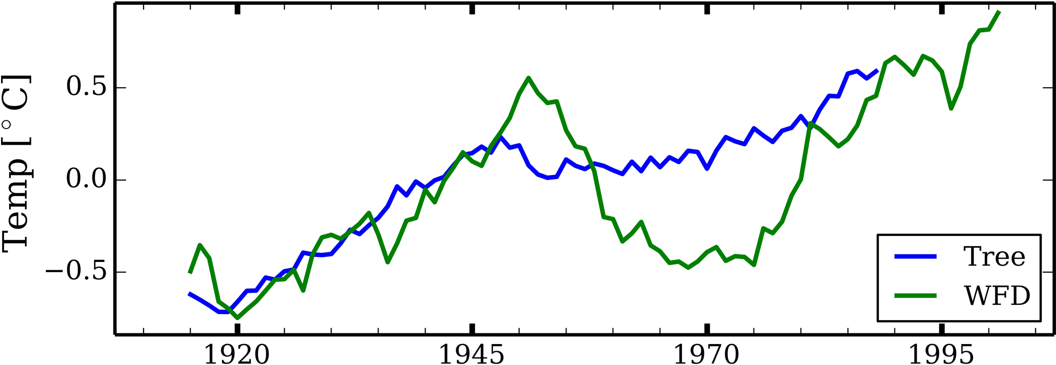
Figure 6Trend comparison of the annual average air temperature data (15-year moving average) based on WCH-FD and tree-ring-based reconstructions.
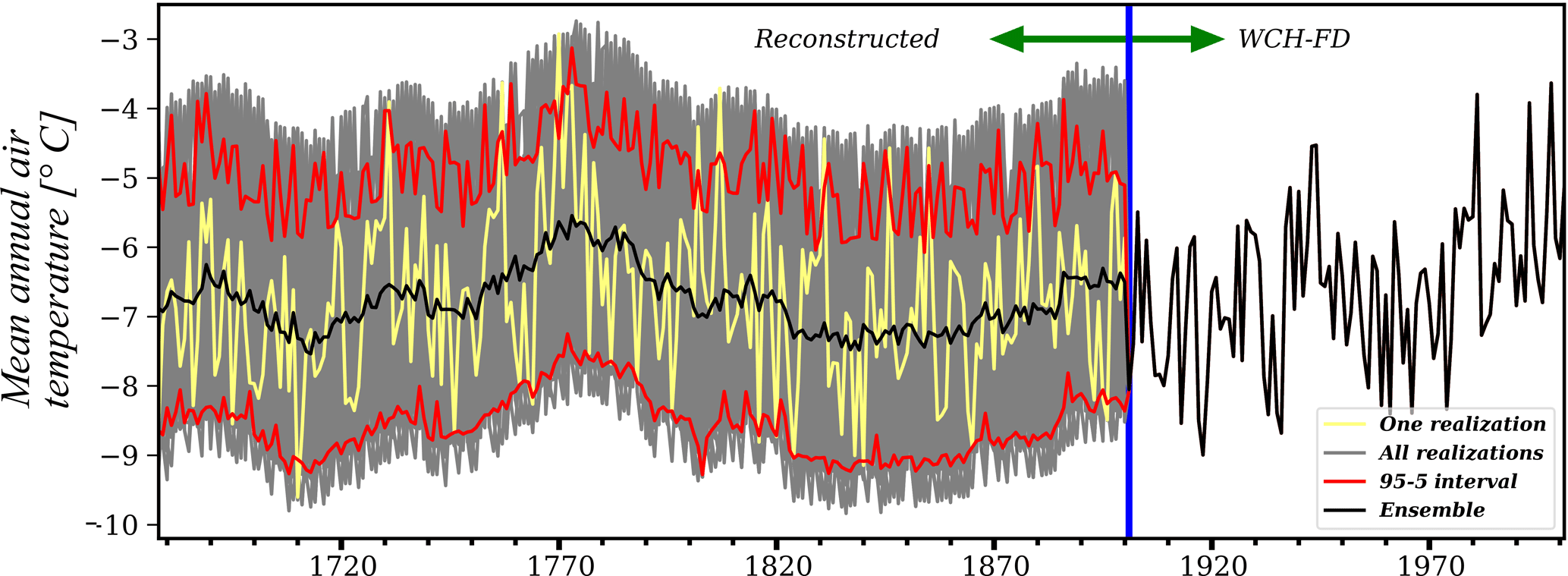
Figure 7Combined air temperature time series generated using the block-bootstrapping technique and WCH-FD. The time series is divided in two periods. From 1678–1900 the temperature and the other six climate variables were generated using the block-bootstrapping technique with a block of 5 years assembled on tree-ring-based reconstructions. The 100 realizations (grey lines), the 5–95 % confidence interval (red lines), and the average of the ensemble (black line) are shown. In the second period (1901–2000) the climate variables are used directly from the WCH-FD database.
To overcome the above challenge, we stochastically generated past climate variables, back to year 1678 based on proxy data of reconstructed summer air temperature described in Sect. 2.1.2. To this end, we applied a block-bootstrapping technique (Razavi et al., 2015; Politis and Romano 1994).
The stochastic time series of climate variables were generated as follows:
-
First, we assumed that the reconstructed summer air temperature by Szeicz and MacDonald (1995) can be used as proxy data to derive the past trends in air temperature. The historical temperature trend back to 1678 (THtrend) was estimated by first computing the moving average with a window of 15 years and then subtracting the moving average from the annual time series. Figure 6 compares both temperature trends (15-year moving average) obtained from WCH-FD data and tree rings for the same period, showing a reasonable agreement, with a Pearson correlation coefficient of 0.66. The existing discrepancy may be in part due to a lack of consideration of longer-term variability (longer than annual) in the reconstruction of the time series, an issue explained in Razavi et al. (2016).
-
Then, we decomposed the WCH-FD temperature time series (6-hourly time resolution) for the period 1901–2001 into its trend (based on the 15-year moving average) and its seasonality component (Tseas).
-
Next, we applied the block-bootstrapping technique with a block size of 5 years to Tseas. We sampled 45 blocks of 5 years so as to generate a time series long enough to cover the 1678–1901 period.
-
To finish the reconstruction of the 6-hourly temperature data, we added Tseas to the THtrend from step (1).
-
The other six climate variables needed by MESH to run were precipitation, shortwave and longwave radiation, specific humidity, wind, and atmospheric pressure. They were generated by applying the block-bootstrapping technique with the same time indexes of the temperature blocks (step 3). In this way, we maintained the interdependence between all the climate variables.
-
Finally, we generated 100 realizations of the climate variables for the period 1678–1901. The complete climate time series of 1678–2000 was finally obtained by combining the generated ones and the WCH-FD data for 1901–2000. Figure 7 shows the mean annual temperature of these 6-hourly time series generated with the methodology presented.
2.5.2 Evaluation procedure
We used the 100 realizations of the climate variables of Sect. 2.5 to run the models with the 50 parameter sets and 17 SCDs used before. For the initial conditions, we used the stabilized model outputs obtained from the 2000 cycles for year 1945 (average with respect to temperature and precipitation). Finally, the simulated soil temperature profiles obtained were compared with the observed data (see Sect. 2.1.1) by computing the root mean squared error (RMSE). To evaluate the model performance in reproducing the observations (1985–2000), individual maximum and minimum soil temperature profiles of simulated and observed data were used to compute RMSE for each individual year. Then all the values of RMSE obtained, one for each year, were averaged to obtain the overall RMSE of the corresponding simulation.
3.1 Soil configuration depth
Using the experiments proposed in Experiment 1, we explored the combined and individual effects of climate, parameters, and SCD on the non-oscillation depth of the soil temperature profile. Figures 8, 9, and 10 summarize these analyses as 2-D histograms: SCD, hT-non-oscillation (Fig. 8); years, hT-non-oscillation (Fig. 9); and parameter sample group, hT-non-oscillation (Fig. 10). Notably, Fig. 8 shows that for SCDs less than 15 m, there is a high probability that the hT-non-oscillation condition is never reached, regardless of the parameter values and the climate conditions (year). For SCDs greater than 20 m, the hT-non-oscillation condition is always reached, with this condition occurring at a higher frequency at a depth between 13 and 16 m.

Figure 8The 2-D histogram of SCD and hT-non-oscillation depth. Counts are normalized by the number of simulations per SCD. The thick black line separates the frequency of reaching and not reaching the hT-non-oscillation conditions; bins to the left of this line are for simulations that never reached the hT-non-oscillation condition.
The variability observed in hT-non-oscillation depth for each SCD is, in general, mainly explained by the variation in parameter values rather than the year selected (i.e., climate condition) for spinning up the model (Figs. 9 and 10).
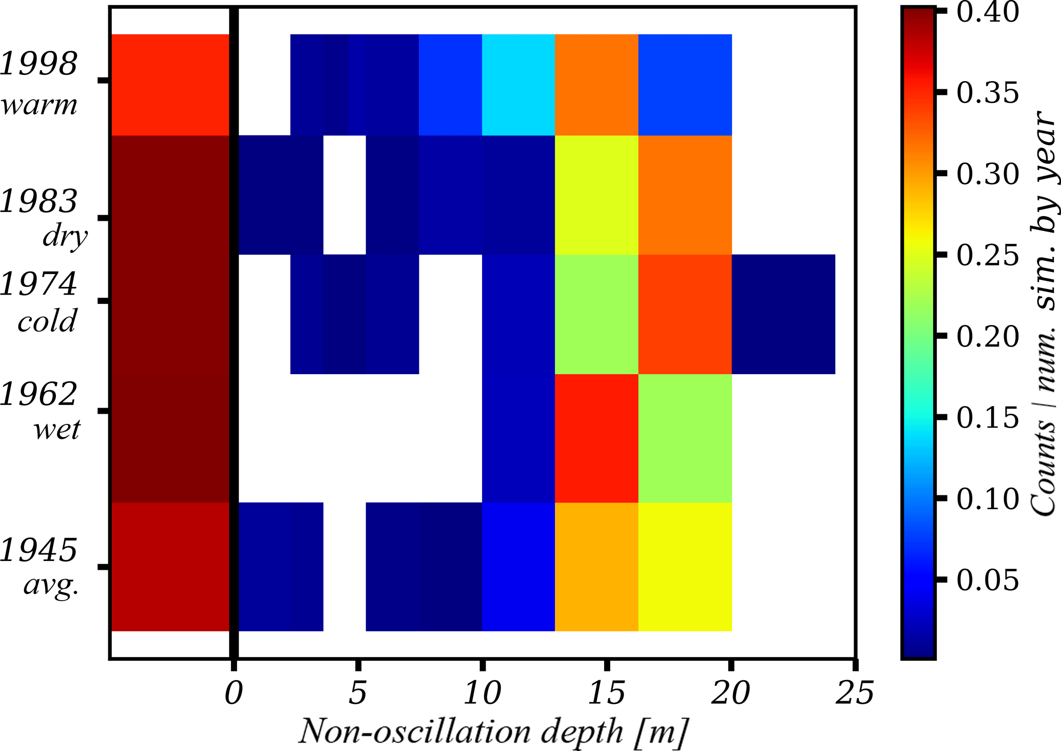
Figure 9The 2-D histogram of climate condition (years) and hT-non-oscillation depth. Counts are normalized by the number of simulations per year. The thick black line separates the frequency of reaching and not reaching the hT-non-oscillation conditions; bins to the left of this line are for simulations that never reached the hT-non-oscillation condition.
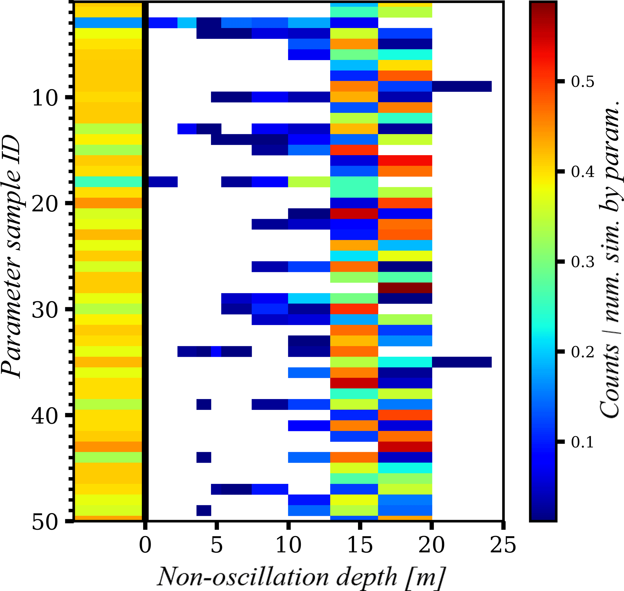
Figure 10The 2-D histogram of parameter and hT-non-oscillation depth. Counts are normalized by the number of simulations by parameter sample. The thick black line separates the frequency of reaching and not reaching the hT-non-oscillation conditions; bins to the left of this line are for simulations that never reached the hT-non-oscillation condition.
From the previous results, it seems clear that we need at least an SCD of greater than 20 m to adequately represent the temperature dynamics of permafrost. This conclusion is supported by the fact that the soil temperature at which hT-non-oscillation condition is reached remains invariant throughout the annual cycle. The distribution of this “non-oscillating temperature” is shown using 2-D histograms in Figs. 11 and 12 with respect to the SCD and the climate conditions (years), respectively.
Figure 11 shows that for shallow SCDs, from 3.1 to 16 m, there is a tendency to obtain a warmer soil temperature such that the permafrost is thawed. In the SCDs with the depth of 16 m and deeper, there is much more variability in the soil temperature (between −6 and 0 ∘C), but with a high probability that the soil temperature at the hT-non-oscillation condition is between −3 and −2.5 ∘C. In Fig. 12 the effect of the climate condition can be appreciated. The main behavioural difference is for the warmest year (1998) when, as expected, the warmest soil temperatures at the hT-non-oscillation condition occur. As for the other climate conditions, the behaviours are quite similar and in general have a range of variation between −7 and 0.5 ∘C. As before (Fig. 11), the probability distribution for each climate condition is quite symmetrical with a peak value around −2.5 ∘C. A slightly cooler soil temperature is obtained for the coldest year (1974).
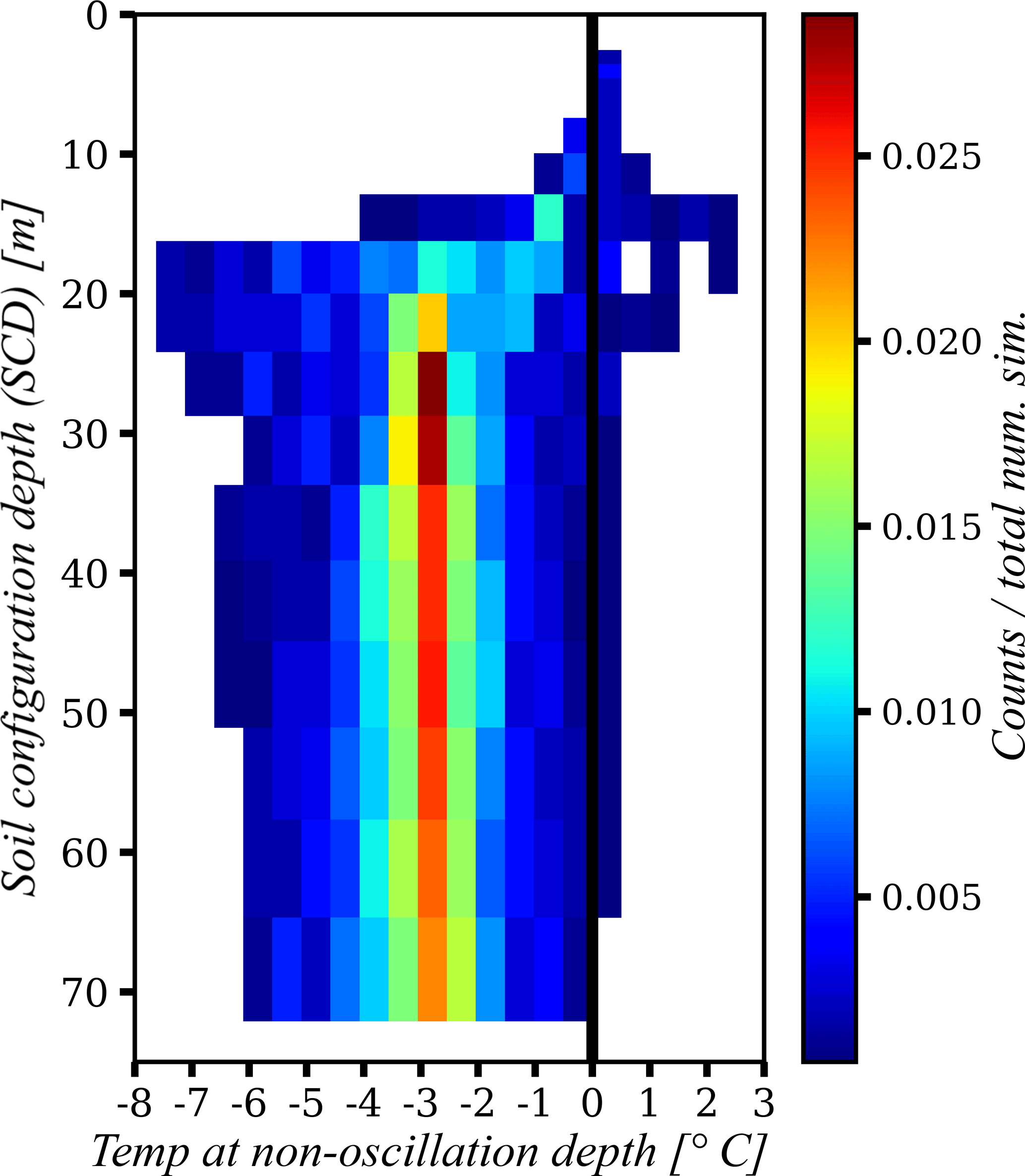
Figure 11The 2-D histogram of SCD and temperature at hT-non-oscillation depth. Only SCDs that have reached the hT-non-oscillation condition are included. The black line represents the 0 ∘C temperature.
3.2 Lower boundary conditions
Figure 13 shows the 2-D histograms (SCD, hT-non-oscillation) for simulations where the geothermal flux is not included (Fig. 13a) and with the geothermal flux (Fig. 13b) in the lower boundary condition. On both experiments the same number of models are run (). The visual comparison indicates that the histogram differences are negligible in most cases. Some marginal differences suggest, as expected, that the models with a constant geothermal flux result in slightly warmer soil profiles and slightly deeper non-oscillation depth compared with no-heat-flow counterparts. These differences are small, and the results confirm that more than 20 m of soil depth are needed to adequately represent the temperature dynamics. To further compare the two scenarios, Fig. 14 shows the cumulative distribution function (CDF) of the differences in soil temperature at the non-oscillation depth of the two simulation scenarios (with and without geothermal flux at the bottom). As shown, the temperature difference of the two scenarios is small in most simulations and is within ±0.15 ∘C in approximately 60 % of simulations.
3.3 Initialization by paleo-reconstructions
The previous sections have shown evidence that, regardless of the climate conditions, parameter uncertainty, and lower boundary conditions, we need to have an SCD that is deeper than 20 m. However, such depths make the model initialization problem challenging. Here, we show the results of our 1-D models with different SCDs and parameter values when driven by a set of 100 tree-ring, bootstrap-based reconstructed climate forcing realizations for the period 1678–2001.
Figure 15a shows a general overview of the model's ability to reproduce the observed soil thermal behaviour between years 1985 and 2000, by plotting the 2-D histogram of SCD and RMSE. The colours for a specific SCD represent the frequency distribution of RMSE values; the variability in this distribution includes the effects of different parameter values and climate forcing realizations. The RMSE was calculated as described in Sect. 2.5.2. In general, for the shallower SCDs (say less than 15 m), the RMSE tends to be larger with a higher variability (1.5 to 9.0 ∘C). The frequency distributions for deeper SCDs become, however, quite similar regardless of the depth, with an RMSE range between 1 and 5 ∘C with a high density around 1.5 to 3.0 ∘C.
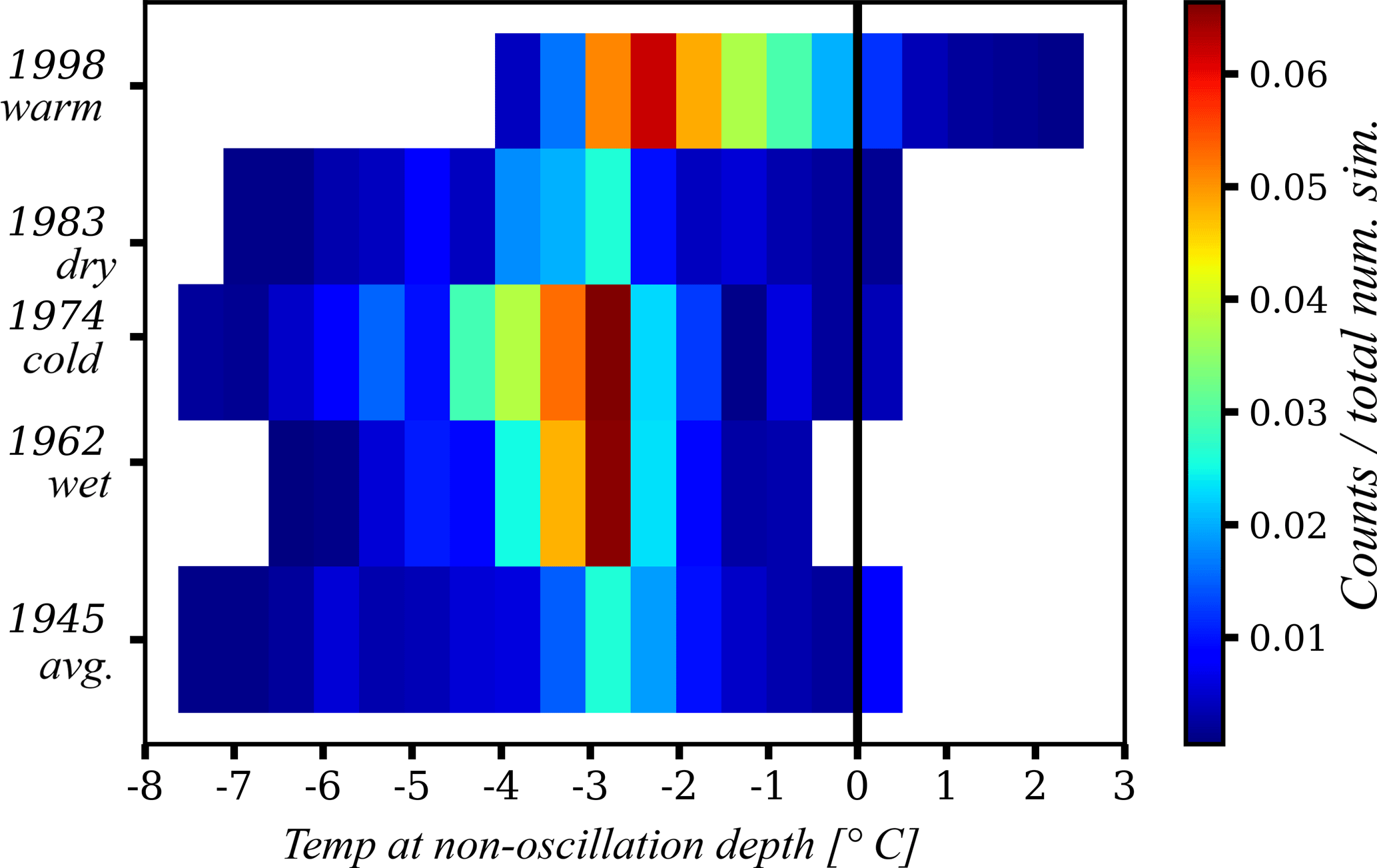
Figure 12The 2-D histogram of climate condition (years) and temperature at hT-non-oscillation depth. Only SCDs that have reached the hT-non-oscillation condition are included. The black line represents the 0 ∘C temperature.
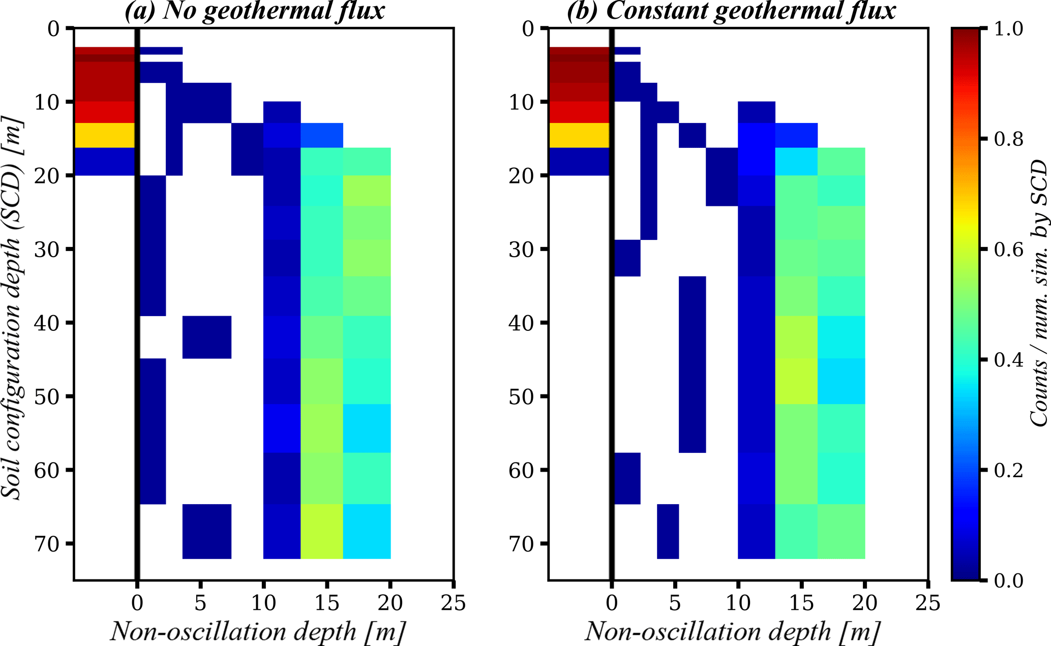
Figure 13The 2-D histogram of SCD and hT-non-oscillation depth. Counts are normalized by the number of simulation by SCD. The black line represents the limit at which the conditions reach or do not the hT-non-oscillation conditions. Bins to the left represent SCDs that never reach the hT-non-oscillation condition. (a) no geothermal flux; (b) constant geothermal flux as lower boundary condition at the bottom of the soil layers.
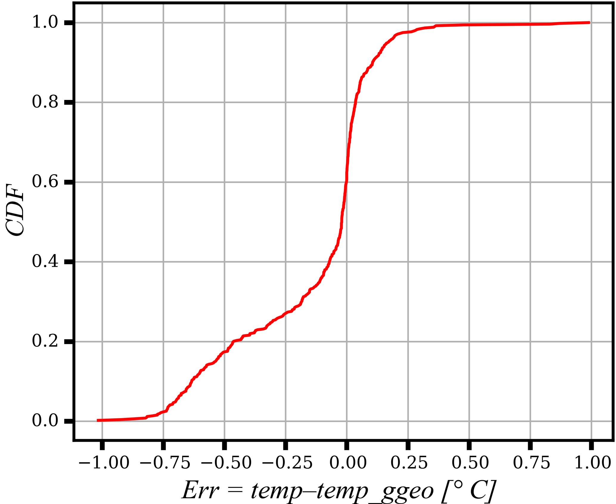
Figure 14Cumulative distribution function (CDF) of the soil temperature difference at the hT-non-oscillation depth between simulations with and without geothermal flux.
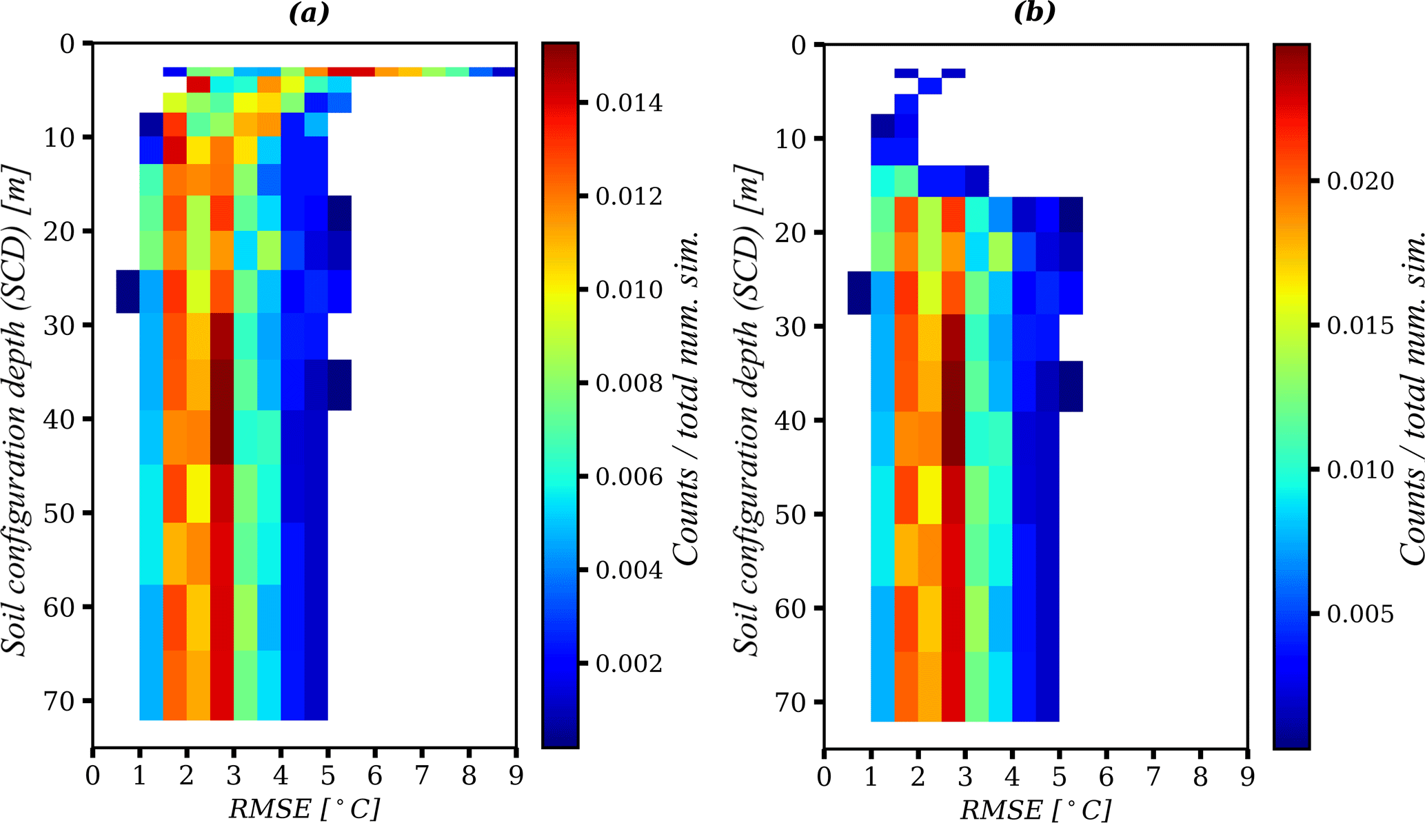
Figure 15The 2-D histograms of SCD and RMSE for the period 1985–2000 when initialized by the bootstrap-based paleo-reconstructions. In plot (a) all the simulations are included, but in plot (b) only the simulations that have reach the hT-non-oscillation condition are included.
In the histogram of Fig. 15a, we included all the simulations, even if in a simulation from Experiment 1 the non-oscillation conditions had not been reached. Figure 15b, however, presents only the simulations that have reached the non-oscillation condition. As can be seen, the histograms of Fig. 15a and b become the same for SCDs deeper than 16 m similar. This is explained by the fact that almost all the simulations with SCDs that are sufficiently deep (> 16.0 m) reach the hT-non-oscillation condition.
Figure 16 shows a series of histograms of RMSE values generated by the different reconstructed climate series, each of which is for a different set of parameter values. This figure is designed to assess the relative effects of the variation in the different reconstructed climate time series (a manifestation of data uncertainty) and variation in model parameters (a manifestation of parameter uncertainty) on the variability of RMSE. Here, we only take into account the simulations that have reached the hT-non-oscillation condition. As can be seen, the range of variation in RMSE for each set of parameter values is quite narrow compared to the union of all the ranges across the different sets of parameter values. Therefore, two points can be made here: (1) the variability observed in RMSE can be attributed mainly to the parameter variations, indicating the significant role of parameter uncertainty; and (2) the effect of stochasticity in the reconstructed time series for the period preceding the period of record is minimal on the model performance in the evaluation period.
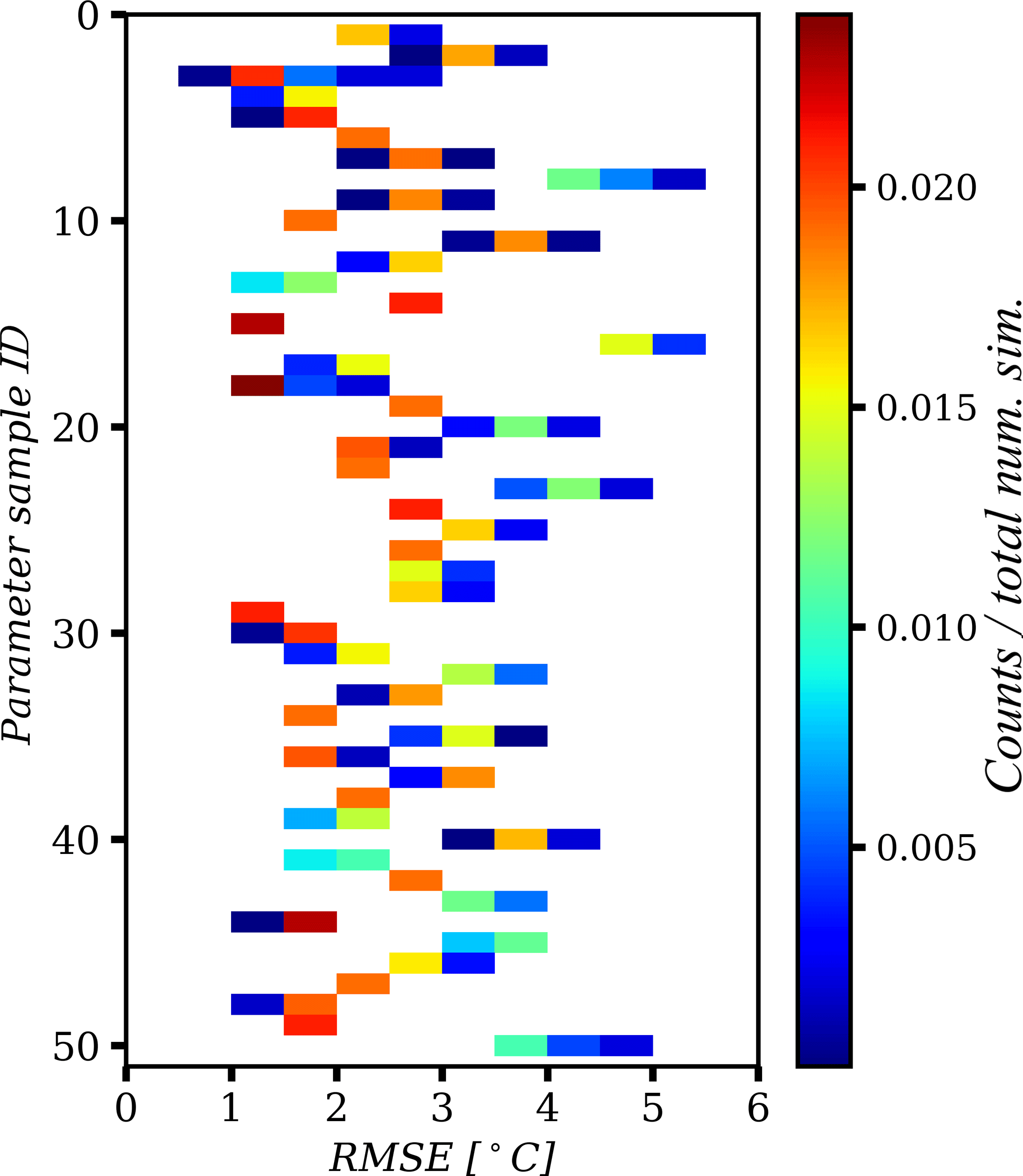
Figure 16The 2-D histogram of parameter sample and RMSE. Only the simulations that reached the hT-non-oscillation condition are included.
This study concludes that for permafrost regions, deeper soil configurations in LSMs are needed than commonly adopted to be able to correctly simulate the coupled energy and water balance in the subsurface. This conclusion can be extended to all Earth system models that incorporate an LSM with permafrost representation. While this conclusion has also been pointed out by other authors, this work investigated the individual and joint effects of parameter uncertainty, total soil depth, lower boundary conditions (geothermal flux), and climate conditions. Further, this work addresses the uncertainty in the reconstructions of past climate for model initialization and also the question of how the initialization should be carried out.
Our analysis shows that the minimum total soil depth should be around 20 m. This value is the reliable depth considering uncertainty and variability in model parameters and climate conditions used to initialize the model and whether or not the geothermal flux is included as lower boundary condition. The metric defined to assess this depth was based on a depth at which the annual maximum and minimum of daily soil temperature are equal, referred to as hT-non-oscillation condition in this paper. This depth represents a thermally stable condition and ensures that the lower boundary condition is deep enough to accommodate a no-heat-flux or constant-heat-flux boundary condition at the bottom of the soil configuration.
The variability observed in the value of hT-non-oscillation across the many simulations we conducted was mainly explained by parameter perturbations rather than climate conditions. This assessment was the case for the both sets of analyses in Experiment 1 and 2. This emphasizes the importance of recognizing and addressing parameter uncertainty and raises serious issues with the common practice in using LSMs with GCMs, where model capabilities are constrained by using hard coded parameters determined based on look-up tables (Mendoza et al., 2015).
We argued that model spin-ups that are based on recycling the 20th century data should be avoided, as simulations on back-to-back repetitions of any sequence of years with a warming trend will result in an unrealistically warm soil temperature profile. Instead, we recommend a two-stage procedure to set the initial conditions of the model: in stage 1 (as conducted in Experiment 1), we spin up the model on an “average” year and then, in stage 2, we further run the model on a multi-century-long bootstrap-based paleo-reconstruction to the beginning of the period of record. The first phase has a stabilizing effect and assures that coherent state variables and fluxes are set before subsequent initialization of the model. This is an important step, as the majority of the LSMs have a large number of state variables to initialize (e.g., CLASS has 17). For the first step, we recommend selecting an average year in terms of air temperature and precipitation, and we recycle that year in simulation until the soil temperature profile is stabilized. Then, in the second step, we recommend using multi-century-long time series of climate variables generated based on the procedure proposed in this study. The proposed procedure reconstructs the time series of temperature using proxy records of summer temperatures derived from tree rings and generates the concurrent time series of other climate variables such as precipitation by applying block bootstrapping on historical records. We were able to reproduce quite well the past trends of summer temperature and we included the effect of uncertainty in the climate time series by generating 100 realizations. An important remark here is that the effect of short-timescale (e.g., annual) fluctuations in the reconstructed time series used for initialization was minimal, while low frequency trends were important. The length of reconstructions required for proper initialization is longer for deeper SCDs.
Finally, we envision our future work being directed to generalize the results obtained here by extending the analyses to other locations where observations of soil profile temperature and past climate are available. Furthermore, implementing a variable SCD in regional and global models may be investigated, as also proposed by Brunke et al. (2016) for the Community Land Model version 4.5. However, the computational burden is a bottleneck for large-scale simulations. To address the computational issues, surrogate modelling strategies that develop cheaper-to-run statistical or mechanistic surrogates of the original models may be explored (Razavi et al., 2012), and also an endeavour may be made by the cryosphere community to generate a unified gridded data set for the last millennium or so (Jungclaus et al., 2017; Landrum et al., 2013; Schmidt et al., 2011) that approximates soil temperature profiles with adequate soil depth, considering the effect of parameter uncertainty via generating ensembles of approximations.
Temperature soil profiles at Normal Wells are available at http://ftp.maps.canada.ca/pub/nrcan_rncan/publications/ess_sst/215/215482/of_4635.zip. Proxy climate records of average summer (June–July) air temperature based on tree rings for the period 1638–1988 are available at ftp://ftp.ncdc.noaa.gov/pub/data/paleo/treering/reconstructions/nwcanada/nwcan-recon.txt.
The authors declare that they have no conflict of interest.
This article is part of the special issue “Understanding and predicting Earth system and hydrological change in cold regions”. It is not associated with a conference.
This research was undertaken as part of the Changing Cold Region Network,
funded by Canada's Natural Science and Engineering Research Council and by
the Canada Excellence Research Chair in Water Security at the University of
Saskatchewan.
Edited by: Sean
Carey
Reviewed by: two anonymous referees
Alexeev, V. A., Nicolsky, D. J., Romanovsky, V. E., and Lawrence, D. M.: An evaluation of deep soil configurations in the CLM3 for improved representation of permafrost, Geophys. Res. Lett., 34, L09502, https://doi.org/10.1029/2007GL029536, 2007.
Bastidas, L. A., Hogue, T. S., Sorooshian, S., Gupta, H. V., and Shuttleworth, W. J.: Parameter sensitivity analysis for different complexity land surface models using multicriteria methods, J. Geophys. Res., 111, D20101, https://doi.org/10.1029/2005JD006377, 2006.
Brunke, M., Broxton, P., Pelletier, J., Gochis, D., Hazenberg, P., Lawrence, D., Leung, L., Niu, G., Troch, P., and Zeng, X.: Implementing and Evaluating Variable Soil Thickness in the Community Land Model, Version 4.5 (CLM4.5). J. Climate, 29, 3441–3461, https://doi.org/10.1175/JCLI-D-15-0307.1, 2016.
Connon, R. F., Quinton, W. L., Craig, J. R., and Hayashi, M.: Changing hydrologic connectivity due to permafrost thaw in the lower Liard River valley, NWT, Canada, Hydrol. Process., 28, 4163–4178, https://doi.org/10.1002/hyp.10206, 2014.
DeBeer, C. M., Wheater, H. S., Quinton, W., Carey, S. K., Stewart, R., MacKay, M., and Marsh, P.: The changing cold regions network: Observation, diagnosis, and prediction of environmental change in the Saskatchewan and Mackenzie River basins, Canada, Sci. China-Earth Sci., 58, 46–60, 2015.
Decharme, B., Martin, E., and Faroux, S.: Reconciling soil thermal and hydrological lower boundary conditions in land surface models, J. Geophys. Res.-Atmos., 118, 7819–7834, https://doi.org/10.1002/jgrd.50631, 2013.
Ednie, M., Wright, J. F., and Duchesne, C.: Establishing initial conditions for transient ground thermal modelling in the Mackenzie Valley: A paleo-climatic reconstruction approach, in: Proceedings, 9th International Conference on Permafrost, Vol. 29, 403–408, 2008.
Esper, J., Cook, E. R., and Schweingruber, F. H.: Low-frequency signals in long tree-ring chronologies for reconstructing past temperature variability, Science, 295, 2250–2253, https://doi.org/10.1126/science.1066208, 2002.
Garland, G. D. and Lennox, D. H.: Heat Flow in Western Canada, Geophys. J. Roy. Astr. S., 6, 245–262, 1962.
Geological Survey of Canada: Canadian Permafrost. Government of Canada, Natural Resources Canada, Earth Sciences Sector; Canada Centre for Mapping and Earth Observation, available at: http://geogratis.gc.ca/api/en/nrcan-rncan/ess-sst/092b663d-198b-5c8d-9665-fa3f5970a14f.html (last access: 5 September 2017), 2000.
Haghnegahdar A., Razavi S., Yassin F., and Wheater H.: Multi-criteria sensitivity analysis as a diagnostic tool for understanding model behavior and characterizing model uncertainty, Hydrol. Process., 31, 4462–4476, https://doi.org/10.1002/hyp.11358, 2017.
Hayashi, M., Goeller, N. T., Quinton, W. L., and Wright, N.: A simple heat-conduction method for simulating the frost-table depth in hydrological models, Hydrol. Process., 21, 2610–2622, 2007.
Hinzman, L. D., Bettez, N. D., Bolton, W. R., Chapin, F. S., Dyurgerov, M. B., Fastie, C. L., Griffith, B., Hollister, R. D., Hope, A., Huntington, H. P., Jensen, A. M., Jia, G. J., Jorgenson, T., Kane, D. L., Klein, D. R., Kofinas, G., Lynch, A. H., Lloyd, A. H.,McGuire, A. D., Nelson, F. E., Oechel, W. C., Osterkamp, T. E., Racine, C. H., Romanovsky, V. E., Stone, R. S., Stow, D. A., Sturm, M., Tweedie, C. E., Vourlitis, G. L., Walker, M. D., Walker, D. A., Webber, P. J., Welker, J. M., Winker, K. S., and Yoshikawa, K.: Evidence and Implications of Recent Climate Change in Northern Alaska and Other Arctic Regions, Climatic Change, 72, 251–298, https://doi.org/10.1007/s10584-005-5352-2, 2005.
IPCC: Climate Change 2013: The Physical Science Basis, Contribution of Working Group I to the Fifth Assessment Report of the Intergovernmental Panel on Climate Change, edited by: Stocker, T. F., Qin, D., Plattner, G.-K., Tignor, M. M. B., Allen, S. K., Boschung, J., Nauels, A., Xia, Y., Bex, V., and Midgley, P. M., Cambridge Univ. Press, 1535 pp., 2013.
Jungclaus, J. H., Bard, E., Baroni, M., Braconnot, P., Cao, J., Chini, L. P., Egorova, T., Evans, M., González-Rouco, J. F., Goosse, H., Hurtt, G. C., Joos, F., Kaplan, J. O., Khodri, M., Klein Goldewijk, K., Krivova, N., LeGrande, A. N., Lorenz, S. J., Luterbacher, J., Man, W., Maycock, A. C., Meinshausen, M., Moberg, A., Muscheler, R., Nehrbass-Ahles, C., Otto-Bliesner, B. I., Phipps, S. J., Pongratz, J., Rozanov, E., Schmidt, G. A., Schmidt, H., Schmutz, W., Schurer, A., Shapiro, A. I., Sigl, M., Smerdon, J. E., Solanki, S. K., Timmreck, C., Toohey, M., Usoskin, I. G., Wagner, S., Wu, C.-J., Yeo, K. L., Zanchettin, D., Zhang, Q., and Zorita, E.: The PMIP4 contribution to CMIP6 – Part 3: The last millennium, scientific objective, and experimental design for the PMIP4 past1000 simulations, Geosci. Model Dev., 10, 4005–4033, https://doi.org/10.5194/gmd-10-4005-2017, 2017.
Landrum, L., Otto-Bliesner, B., Wahl, E., Conley, A., Lawrence, P., Rosenbloom, N., and Teng, H.: Last Millennium Climate and Its Variability in CCSM4, J. Climate, 26, 1085–1111, https://doi.org/10.1175/JCLI-D-11-00326.1, 2013.
Lawrence, D. M. and Slater, A. G.: A projection of severe near-surface permafrost degradation during the 21st century, Geophys. Res. Lett., 32, L24401, https://doi.org/10.1029/2005GL025080, 2005.
Lawrence, D. M., Slater, A. G., Romanovsky, V. E., and Nicolsky, D. J.: Sensitivity of a model projection of near-surface permafrost degradation to soil column depth and representation of soil organic matter, J. Geophys. Res., 113, F02011, https://doi.org/10.1029/2007JF000883, 2008.
Marshall, S.: Glacier retreat crosses a line, Science, 345, p. 872, https://doi.org/10.1126/science.1258584, 2014.
Mekonnen, M. A., Wheater, H. S., Ireson, A. M., Spence, C., Davison, B., and Pietroniro, A.: Towards an Improved Land Surface Scheme for Prairie Landscapes, J. Hydrol., 511, 105–116, https://doi.org/10.1016/j.jhydrol.2014.01.020, 2014.
Mendoza, P. A., Clark, M. P., Barlage, M., Rajagopalan, B., Samaniego, L., Abramowitz, G., and Gupta, H.: Are we unnecessarily constraining the agility of complex process-based models?, Water Resour. Res., 51, 716–728, https://doi.org/10.1002/2014WR015820, 2015.
Nicolsky, D. J., Romanovsky, V. E., Alexeev, V. A., and Lawrence, D. M.: Improved modeling of permafrost dynamics in a GCM land-surface scheme, Geophys. Res. Lett., 34, L08501, https://doi.org/10.1029/2007GL029525, 2007.
Paquin, J. P. and Sushama, L.: On the Arctic near-surface permafrost and climate sensitivities to soil and snow model formulations in climate models, Clim. Dynam., 44, 203–228, https://doi.org/10.1007/s00382-014-2185-6, 2015.
Peel, M. C., Finlayson, B. L., and McMahon, T. A.: Updated world map of the Köppen-Geiger climate classification, Hydrol. Earth Syst. Sci., 11, 1633–1644, https://doi.org/10.5194/hess-11-1633-2007, 2007.
Pietroniro, A., Fortin, V., Kouwen, N., Neal, C., Turcotte, R., Davison, B., Verseghy, D., Soulis, E. D., Caldwell, R., Evora, N., and Pellerin, P.: Development of the MESH modelling system for hydrological ensemble forecasting of the Laurentian Great Lakes at the regional scale, Hydrol. Earth Syst. Sci., 11, 1279–1294, https://doi.org/10.5194/hess-11-1279-2007, 2007.
Politis, D. N. and Romano, J. P.: The stationary bootstrap, J. Am. Stat. Assoc., 89, 1303–1313, 1994.
Razavi, S. and Gupta, H. V.: What do we mean by sensitivity analysis? The need for comprehensive characterization of “global” sensitivity in Earth and Environmental systems models, Water Resour. Res., 51, 3070–3092, https://doi.org/10.1002/2014WR016527, 2015.
Razavi, S., Tolson, B. A., and Burn, D. H.: Review of surrogate modelling in water resources, Water Resour. Res., 48, W07401, https://doi.org/10.1029/2011WR011527, 2012.
Razavi, S., Elshorbagy, A., Wheater, H., and Sauchyn, D.: Toward understanding nonstationarity in climate and hydrology through tree ring proxy records, Water Resour. Res., 51, 1813–1830, https://doi.org/10.1002/2014WR015696, 2015.
Razavi, S., Elshorbagy, A., Wheater, H., and Sauchyn, D.: Time scale effect and uncertainty in reconstruction of Paleo-hydrology, Hydrol. Process., 30, 1985–1999. https://doi.org/10.1002/hyp.10754, 2016.
Rodell, M., Houser, P. R., Berg, A. A., and Famiglietti, J. S.: Evaluation of 10 Methods for Initializing a Land Surface Model, J. Hydrometeorol., 6, 146–155, https://doi.org/10.1175/JHM414.1, 2005.
Rowland, J. C., Jones, C. E., Altmann, G., Bryan, R., Crosby, B. T., Geernaert, G. L., Hinzman, L. D., Kane, D. L., Lawrence, D. M., Mancino, A., Marsh, P., McNamara, J. P., Romanovsky, V. E., Toniolo, H., Travis, J., Trochim, E., and Wilson, C. J. : Arctic landscapes in transition: Responses to thawing permafrost, Eos, 91, 229–230, 2010.
Schmidt, G. A., Jungclaus, J. H., Ammann, C. M., Bard, E., Braconnot, P., Crowley, T. J., Delaygue, G., Joos, F., Krivova, N. A., Muscheler, R., Otto-Bliesner, B. L., Pongratz, J., Shindell, D. T., Solanki, S. K., Steinhilber, F., and Vieira, L. E. A.: Climate forcing reconstructions for use in PMIP simulations of the last millennium (v1.0), Geosci. Model Dev., 4, 33–45, https://doi.org/10.5194/gmd-4-33-2011, 2011.
Schuur, E. A. G., McGuire, A. D., Schädel, C., Grosse, G., Harden, J. W., Hayes, D. J., Hugelius, G., Koven, C. D., Kuhry, P., Lawrence, D. M., Natali, S. M., Olefeldt, D., Romanovsky, V. E., Schaefer, K., Turetsky, M. R., Treat, C. C., and Vonk, J. E.: Climate change and the permafrost carbon feedback, Nature, 250, 171–178, 2015.
Shrestha, R. and Houser, P.: A heterogeneous land surface model initialization study, J. Geophys. Res., 115, D19111, https://doi.org/10.1029/2009JD013252, 2010.
Slater, A. G. and Lawrence, D. M.: Diagnosing present and future permafrost from climate models, J. Climate, 26, 5608–5623, 2013.
Smith, S. L., Burgess, M. M., Riseborough, D., Coultish, T., and Chartrand, J.: Digital summary database of permafrost and thermal conditions - Norman Wells Pipeline study sites; Geological Survey of Canada, Open File 4635, 104 pp., 2004.
Soulis, E. D., Snelgrove, K. R., Kouwen, N., Seglenieks, F., and Verseghy, D. L. Towards closing the vertical water balance in Canadian atmospheric models: Coupling of the land surface scheme class with the distributed hydrological model watflood, Atmos. Ocean, 38, 251–269, https://doi.org/10.1080/07055900.2000.9649648, 2000.
Stevens, M. B., Smerdon, J. E., González-Rouco, J. F., Stieglitz, M., and Beltrami, H.: Effects of bottom boundary placement on subsurface heat storage: Implications for climate model simulations, Geophys. Res. Lett., 34, L02702, https://doi.org/10.1029/2006GL028546, 2007.
Sturm, M., Racine, C., and Tape, K.: Climate change: increasing shrub abundance in the Arctic, Nature, 411, 546–547, 2001.
Szeicz, J. M. and MacDonald, G. M.: Dendroclimatic reconstruction of Summer Temperatures in northwestern Canada Since AD 1638 Based on Age-Dependent Modeling, Quaternary Res., 44, 257–266, 1995.
Troy, T. J., Sheffield, J., and Wood, E. F.: The role of winter precipitation and temperature on northern Eurasian streamflow trends, J. Geophys. Res., 117, D05131, https://doi.org/10.1029/2011JD016208, 2012.
Verseghy, D.: CLASS – The Canadian Land Surface Scheme (Version 3.4), Technical Documentation (Version 1.1), Climate Research Division, Science and Technology Branch, Environment Canada, 180 pp., 2009.
Verseghy, D. L.: CLASS – A Canadian land surface scheme for GCMs, I. Soil model, Int. J. Climatol., 11, 111–133, 1991.
Verseghy, D. L., McFarlane, N. A., and Lazare, M.: Class – A Canadian land surface scheme for GCMS, II. Vegetation model and coupled runs, Int. J. Climatol., 13, 347–370, https://doi.org/10.1002/joc.3370130402, 1993.
Weedon, G., Gomes, S., Viterbo, P., Shuttleworth, W., Blyth, E., Österle, H., Adam, J., Bellouin, N., Boucher, O., and Best, M.: Creation of the WATCH Forcing Data and Its Use to Assess Global and Regional Reference Crop Evaporation over Land during the Twentieth Century, J. Hydrometeorol., 12, 823–848, https://doi.org/10.1175/2011JHM1369.1, 2011.
Woo, M.: Permafrost Hydrology, Springer, New York, 572 pp., 2012.
Yang, Z.-L., Dickinson, R. E., Henderson-Sellers, A., and Pitman, A. J.: Preliminary study of spin-up processes in land surface models with the first stage data of Project for Intercomparison of Land Surface Parameterization Schemes Phase 1(a), J. Geophys. Res., 100, 16553–16578, https://doi.org/10.1029/95JD01076, 1995.
Yassin, F., Razavi, S., Wheater, H., Sapriza-Azuri, G., Davison, B., and Pietroniro, A.: Enhanced identification of a hydrologic model using streamflow and satellite water storage data: A multicriteria sensitivity analysis and optimization approach, Hydrol. Process., 31, 3320–3333, https://doi.org/10.1002/hyp.11267, 2017.
Zhang, Y., Chen, W., and Cihlar, J.: A process-based model for quantifying the impact of climate change on permafrost thermal regimes, J. Geophys. Res., 108, 4695, https://doi.org/10.1029/2002JD003354, 2003.
Zhang, Y., Chen, W., and Riseborough, D. W.: Temporal and spatial changes of permafrost in Canada since the end of the Little Ice Age, J. Geophys. Res., 111, D22103, https://doi.org/10.1029/2006JD007284, 2006.
Zhang, Y., Chen, W., and Riseborough, D. W.: Disequilibrium response of permafrost thaw to climate warming in Canada over 1850–2100, Geophys. Res. Lett., 35, L02502, https://doi.org/10.1029/2007GL032117, 2008.