Hydro-stochastic interpolation coupling with the Budyko approach for prediction of mean annual runoff

The hydro-stochastic interpolation method based on traditional block Kriging has often been used to predict mean annual runoff in river basins. A caveat in such a method is that the statistic technique provides little physical insight into relationships between the runoff and its external forcing, such as the climate and land cover. In this study, the spatial runoff is decomposed into a deterministic trend and deviations from it caused by stochastic fluctuations. The former is described by the Budyko method (Fu's equation) and the latter by stochastic interpolation. This coupled method is applied to spatially interpolate runoff in the Huaihe River basin of China. Results show that the coupled method significantly improves the prediction accuracy of the mean annual runoff. The error of the predicted runoff by the coupled method is much smaller than that from the Budyko method and the hydro-stochastic interpolation method alone. The determination coefficient for cross-validation, $R_{\mathrm{cv}}^{\mathrm{2}}$, from the coupled method is 0.87, larger than 0.81 from the Budyko method and 0.71 from the hydro-stochastic interpolation. Further comparisons indicate that the coupled method has also reduced the error in overestimating low runoff and underestimating high runoff suffered by the other two methods. These results confirm that the coupled method offers an effective and more accurate way to predict the mean annual runoff in river basins.

1 Introduction

The runoff observed at the outlet of a basin is a crucial element for investigating the hydrological cycle of the basin. Because runoff is influenced by both deterministic and stochastic processes, estimating the spatial patterns of runoff and the associated distribution of water resources in ungauged basins has been one of the key problems in hydrology (Sivapalan et al., 2003), and a thorny issue in water management and planning (Imbach, 2010; Greenwood et al., 2011).

In estimating and predicting runoff and regional water resources availability, we have often used regional or global runoff mapping and geostatistical interpolation methods. In these methods, the value of a regional variable at a given location is often estimated as the weighted average of observed values at neighboring locations. This interpolation of runoff, which is assumed as an auto-correlated generalized stochastic field (Jones, 2009), uses secondary information from more than one variable (Li and Heap, 2008). Spatial autocorrelations of the runoff values are measured by the covariance or semi-variance between the runoffs at pairs of locations as a function of their Euclidian distance (such as in ordinary Kriging). The values obtained by the interpolation methods are the best linear unbiased estimate in the sense that the expected bias is zero and the mean squared error is minimized (Skøien et al., 2006). Ordinary Kriging (OK) estimates the local mean as a constant; corresponding residuals are considered random. Because the spatial mean could also be used as a trend or nonstationary variation in space, OK has been developed into various geostatistical interpolation methods, such as Kriging with a trend by incorporating a local trend within a confined neighborhood as a smoothly varying function of the coordinates. Block Kriging (BK) is another extension of OK for estimating a block value instead of a point value by replacing the point-to-point covariance with point-to-block covariance (Wackernagel, 1995).

Unlike precipitation or evaporation, which we often interpolate to find their values at specific locations, runoff is an integrated spatially continuous process in river basins (Lenton and Rodriguez-Iturbe, 1977; Creutin and Obled, 1982; Tabios and Salas, 1985; Dingman et al., 1988; Barancourt et al., 1992; Blöschl, 2005). Streamflows are naturally organized into basins (Dooge, 1986; Sivapalan, 2005); e.g., rivers flow through sub-basins. The river network constrains the water paths from upstream to downstream in a basin. The hierarchically organized river network requires that the sum of the interpolated discharge from sub-basins equals the observed runoff at the outlet of the entire basin. Previous studies have indicated that runoff interpolation may overestimate the actual runoff without adequate information of the spatial variation of the runoff (Arnell, 1995), e.g., neglecting the river network in connecting sub-basins or processing basin runoff at collective points in space (Villeneuve et al., 1979; Hisdal and Tveito, 1993). In nested basins, Gottschalk (1993a, b) developed a hydro-stochastic method to interpolate runoff. It uses the concept that runoff is an integrated process in the hierarchical structure of a river network. The distance between a pair of basins is measured by geostatistical distance instead of the Euclidian distance. The covariogram among points in the conventional spatial interpolation is replaced by the covariogram between basins. In this concept, runoff is assumed spatially homogeneous in basins; i.e., the expected value of the runoff is constant in space (Sauquet, 2006). The observed patterns of runoff reveal systematic deviations from the homogeneity assumption, however, because of the influences from the heterogeneous climate and underlying surface factors.

An alternate method is to describe the hydrological variables of interest in deterministic forms of functions, curves, or distributions, and construct conceptual and mathematical models to predict hydro-climate variability (Wagener et al., 2007). Qiao (1982), Arnell (1992), and Gao et al. (2017) have used such an approach and derived empirical relationships between runoff and its controlling factors of the climate, land cover, and topography in various basins. However, the deterministic method for describing complex runoff patterns suffers from an inevitable loss of information (Wagener et al., 2007) because of the existence of uncertainty in many hydrological processes and especially in observations. Thus, hydrological variables also contain information of a stochastic nature and should be treated as outcomes from deterministic and stochastic processes. A method that combines both deterministic patterns and stochastic variability is Kriging with an external drift (KED) (Goovaerts, 1997; Li and Heap, 2008; Laaha et al., 2013). It takes the deterministic patterns of spatial variables into account and incorporates them as a local trend of a smoothly varying secondary variable, instead of a function of the spatial coordinates.

The inclusion of deterministic terms in the geostatistical methods has been shown to increase the interpolation accuracy of basin variables, such as mean annual runoff (Sauquet, 2006), stream temperature (Laaha et al., 2013), and groundwater table (Holman et al., 2009). Those deterministic terms are often described by empirical formulae linking spatial features, e.g., variability of the mean annual runoff in elevation (Sauquet, 2006), and the relationship between the mean annual stream temperature and the altitude of gauges (Laaha et al., 2013). As a semi-empirical approach to model the deterministic process of the runoff, the Budyko framework has been popularly used to analyze the relationship between mean annual runoff and the climatic factors, e.g., aridity index (Milly, 1994; Koster and Suarez, 1999; Zhang et al., 2001; Donohue et al., 2007; Li et al., 2013; Greve et al., 2014). Many efforts have been devoted to improving the Budyko method by, for example, including the effects of other external forcing factors, such as land cover (Donohue et al., 2007, 2012; Li et al., 2013; Han et al., 2011; Yang et al., 2007), soil properties (Porporato et al., 2004), topography (Shao et al., 2012; Xu et al., 2013; Gao et al., 2017), hydro-climatic variations of seasonality (Milly, 1994; Gentine et al., 2012; Berghuijs et al., 2014), and groundwater (Istanbulluoglu et al., 2012). However, it has been found that the use of the deterministic equation in the Budyko method alone still comes with large errors in the prediction of runoff in many basins (e.g., Potter and Zhang, 2009; Jiang et al., 2015).

The aim of this study is to combine the stochastic interpolation with the semi-empirical Budyko method to further improve the spatial interpolation/prediction of the mean annual runoff in the Huaihe River basin (HRB), China. In this study, the spatial runoff from sub-basins in the HRB is separated into a deterministic trend and its residuals, which are estimated by the Budyko method and the interpolation method, respectively. The residuals are calculated as the difference between the observed and estimated runoff from the Budyko method, and are used in the stochastic interpolation as described in Gottschalk (1993a, b, 2006). After that, the runoff of any sub-basin is predicted as the sum of the interpolated residuals and the Budyko estimated value. The improved method is tested in the HRB. In addition, the leave-one-out cross-validation approach is applied to evaluate and compare the performances of the three interpolation methods: the Budyko method, hydro-stochastic interpolation, and our coupled Budyko and stochastic interpolation method.

2 Methodologies

2.1 Spatial estimation of mean annual runoff by the Budyko method

The Budyko method explains the variability of mean annual water balance on a regional or global scale. It describes the dependence of actual evapotranspiration (E) on precipitation (P) and potential evapotranspiration (E₀) (Williams et al., 2012). Their original relationship ($E/P\sim E_{\mathrm{0}}/P$) derived by Budyko (1974) is deterministic and nonparametric. It was later developed into parametric forms (Fu, 1981; Choudhury, 1999; Yang et al., 2008; Gerrits et al., 2009; Wang and Tang, 2014). Among them, the one-parameter equation derived by Fu (1981) and Zhang et al. (2004) has been used frequently. This relationship is written as

$$\begin{array}{}\text{(1)}& {\displaystyle \frac{E}{P}}=\mathrm{1}+{\displaystyle \frac{E_{\mathrm{0}}}{P}}-{\left(\mathrm{1}+{\left({\displaystyle \frac{E_{\mathrm{0}}}{P}}\right)}^{\mathit{\omega }}\right)}^{\frac{\mathrm{1}}{\mathit{\omega }}}\end{array}$$

or

$$\begin{array}{}\text{(2)}& R=P{\left(\mathrm{1}+{\left({\displaystyle \frac{E_{\mathrm{0}}}{P}}\right)}^{\mathit{\omega }}\right)}^{\frac{\mathrm{1}}{\mathit{\omega }}}-E_{\mathrm{0}},\end{array}$$

where P, E, E₀, and R are mean annual precipitation, actual evapotranspiration, potential evapotranspiration, and runoff (units: mm), respectively, and ω is a dimensionless model parameter in the range of (1,∞). In these formulae, the larger the ω is, the smaller the partition of precipitation into the runoff.

The parameter ω in Eq. (1) is determined using observed P, E₀, and R in gauged sub-basins. The mean value of ω of a basin can be obtained by averaging ω of the sub-basins, or by minimizing the mean absolute error (MAE) in fitting the curve in Eq. (1) with $E/P\sim E_{\mathrm{0}}/P$ ($E=P-R$) (Legates and McCabe, 1999). Using the mean value of ω, Eq. (2) can be used to predict ungauged basin runoff or to interpolate the spatial variation of the runoff, using meteorological data in targeted sub-basins (Parajka and Szolgay, 1998).

2.2 Hydro-stochastic interpolation method

Gottschalk (1993a) described the hydro-stochastic interpolation method based on the Kriging method to predict spatial runoff. Gottschalk's method redefines a relevant distance between basins, and identifies the river network and supplemental water balance constraints as follows.

As a spatially integrated continuous process, the predicted runoff of a specific unit of an area A₀ in a basin, r^*(A₀), can be expressed as

$$\begin{array}{}\text{(3)}& r^{*}\left(A_{\mathrm{0}}\right)={\sum }_{i=\mathrm{1}}^n{\mathit{\lambda }}_{i}r\left(A_i\right),\end{array}$$

where r(A_i) is the observed runoff in a gauged basin i with area A_i ($i=\mathrm{1},\mathrm{\dots }n$; n is the total number of gauged basins), and λ_i is the weight of basin i.

The weights are obtained by solving the following set of equations under the second-order stationary assumption for hydrologic variables (Ripley, 1976),

$$\begin{array}{}\text{(4)}& \left\{\begin{array}{l}{\sum }_{j=\mathrm{1}}^n{\mathit{\lambda }}_i\mathrm{Cov}\left(u_i,u_j\right)+\mathit{\mu }=\mathrm{Cov}\left(u_i,u_{\mathrm{0}}\right),\\ i,j=\mathrm{1},\mathrm{2},\mathrm{\dots },n\\ {\sum }_{i=\mathrm{1}}^n{\mathit{\lambda }}_i=\mathrm{1}.\end{array}\right.\end{array}$$

In Eq. (4), Cov(u_i,u_j) is the theoretical covariance function between each pair of gauged stations (i=1, …, n, j= 1, 2, …, n), Cov(u_i,u₀) is the theoretical covariance of runoff between the location of interest u₀ and each of the gauged stations u_i, and μ is the Lagrange multiplier.

The sum of the interpolated runoff for each non-overlapping sub-basin should be equal to the observed runoff at the river outlet. This constraint can be written as

$$\begin{array}{}\text{(5)}& R_T={\sum }_{i=\mathrm{1}}^M\mathrm{\Delta }{A}_{i}r\left(\mathrm{\Delta }{A}_i\right)\end{array}$$

where R_T is the streamflow observed at the outlet of the basin, ΔA_i is the non-overlapping area of sub-basin i, and r(ΔA_i) is the runoff depth for sub-basin i ($i=\mathrm{1},\mathrm{\dots },M$). The predicted runoff for each ΔA_i is a linear combination of the weights and the runoff observed in the n sub-basins, i.e., $r\left(\mathrm{\Delta }{A}_i\right)={\sum }_{j=\mathrm{1}}^n{\mathit{\lambda }}_j^{i}r\left(A_j\right)$. Substituting it in Eq. (5), we get

$$\begin{array}{}\text{(6)}& R_T={\sum }_{i=\mathrm{1}}^M\mathrm{\Delta }{A}_i\left({\sum }_{j=\mathrm{1}}^n{\mathit{\lambda }}_j^{i}r\left(A_j\right)\right).\end{array}$$

In Eq. (6),  r(A_j) is the runoff depth for sub-basin j (j= 1, …, n) with discharge observations, and ${\mathit{\lambda }}_j^i$ is the weight (i= 1, …, M; j= 1, …, n). Further considering the basin area in the river network, Sauquet et al. (2000) derived the weight matrices and described a hydro-stochastic method to optimize the weights ${\mathit{\lambda }}_j^i$ (i=1, …, M; j=1, …, n) in Eq. (6).

The theoretical covariogram, Cov(AB), is derived by averaging the point process covariance function Cov_p

$$\begin{array}{}\text{(7)}& \mathrm{Cov}\left(\mathrm{AB}\right)={\displaystyle \frac{\mathrm{1}}{\mathrm{AB}}}\int \underset{\mathrm{AB}}{\int }{\mathrm{Cov}}_{\mathrm{p}}(\mathrm{|}\mathrm{|}{u}_{\mathrm{1}}-u_{\mathrm{2}}\mathrm{|}\mathrm{|})d{u}_{\mathrm{1}}d{u}_{\mathrm{2}}\end{array}$$

where Cov_p(||u₁−u₂||) is the theoretical covariance function value of pairs of points in basins A and B with distance $d=\mathrm{|}\mathrm{|}{u}_{\mathrm{1}}-u_{\mathrm{2}}\mathrm{|}\mathrm{|}$.

The distance d(AB) is calculated based on grid division in each of the sub-basins (Sauquet et al., 2000). The trial-and-error fitting method is used to calibrate Cov_p(d) in Eq. (7) to best fit Cov_e(d). Only independent sub-basins are used to calculate the covariance function to avoid spatial correlation of nested sub-basins.

2.3 Coupling the stochastic interpolation with the Budyko method

The above stochastic interpolation procedure assumes a stationary stochastic variation of the runoff among sub-basins or spatial homogeneity in runoff (Sauquet, 2006), despite variations in river networks. For nonstationary variations in the runoff resulting from spatial heterogeneity in a river network, the spatial runoff can be decomposed into a nonstationary deterministic component and a stochastic component:

$$\begin{array}{}\text{(8)}& R\left(x\right)=R_{\mathrm{d}}\left(x\right)+R_{\mathrm{s}}\left(x\right).\end{array}$$

In Eq. (8), R(x) is the runoff at a location x, and R_d(x) is the deterministic component of the spatial trend or the external drift (Wackernagel, 1995) that results in nonstationary variability in space. R_s(x) is the stochastic component considered to be stationary.

In this study, R in Eq. (2) is used as an external drift function in estimating the R_d(x) in all sub-basins; i.e., R_d(x) in Eq. (8) is substituted in Eq. (2) by setting R_d(x)=R. The residuals between R_d(x) and the observed runoff are calculated for all gauged sub-basins. Furthermore, these residuals are interpolated for all ungauged sub-basins and set as the stochastic component R_s(x) in Eq. (8) using the “residual kriging” method (Sauquet, 2006). In particular, R_s(x) in Eq. (8) is replaced by r^*(A₀) in Eq. (3) after setting $r^{*}\left(A_{\mathrm{0}}\right)=R_{\mathrm{s}}\left(x\right)$ for the stochastic interpolation scheme described in Sect. 2.2. The superposition of these estimates of both components on the right-hand side in Eq. (8) yields the prediction of R(x).

2.4 Cross-validation

To validate this prediction procedure, we use the leave-one-out cross-validation method (Kearns and Ron, 1999). In addition to quantifying the performance of our coupled Budyko and hydro-stochastic interpolation method, we compare and contrast its performance with the Budyko and hydro-stochastic interpolation methods alone. Their performances are evaluated by the following metrics (Laaha and Blöschl, 2006):

$$\begin{array}{}\text{(9)}& {\displaystyle }& {\displaystyle }\mathrm{MAE}={\displaystyle \frac{\mathrm{1}}{n}}{\sum }_{j=\mathrm{1}}^n\left[R\left(x_i\right)-R^{*}\left(x_i\right)\right],\text{(10)}& {\displaystyle }& {\displaystyle }\mathrm{MSE}={\displaystyle \frac{\mathrm{1}}{n}}{\sum }_{j=\mathrm{1}}^n{\left[R\left(x_i\right)-R^{*}\left(x_i\right)\right]}^{\mathrm{2}},\text{(11)}& {\displaystyle }& {\displaystyle }\mathrm{RMSE}=\sqrt{{\displaystyle \frac{\mathrm{1}}{n}}{\sum }_{j=\mathrm{1}}^n{\left[R\left(x_i\right)-R^{*}\left(x_i\right)\right]}^{\mathrm{2}}},\end{array}$$

where R^*(x) and R(x) are the predicted and observed runoff, respectively, MAE is the mean absolute error, MSE is the mean-square error, and RMSE is the root-mean-square error. The determination coefficient for cross-validation is

$$\begin{array}{}\text{(12)}& R_{\mathrm{cv}}^{\mathrm{2}}=\mathrm{1}-{\displaystyle \frac{V_{\mathrm{cv}}}{V_{\mathrm{NK}}}}\end{array}$$

where V_cv is the MSE, and V_NK is the spatial variance ($V_{\mathrm{NK}}=\frac{{\sum }_{j=\mathrm{1}}^n{\left[R\left(x_i\right)-\stackrel{\mathrm{‾}}{R}\right]}^{\mathrm{2}}}{n-\mathrm{1}}$, in which $\stackrel{\mathrm{‾}}{R}$ is the mean R(x)) of the runoff over all of the tested sub-basins. In addition to these evaluation metrics, the prediction result is evaluated by regression analysis of the observation vs. the prediction.

3 Study catchment and data

The HRB, the sixth largest river basin in China, is used in evaluation of our coupled model and in its comparison to the other two methods. The HRB has a strong precipitation gradient from the humid climate in the east and the semi-humid climate in the west (Hu, 2008). It is one of the major agricultural areas in China, with the highest human population density in the country. About 18 billion m³ of water was consumed in 1998 to meet the basin's domestic and agriculture needs. Water resources per capita and per unit area are less than one-fifth of the national average. Moreover, more than 50 % of the water resources are exploited, much higher than the recommended 30 % for inland river basins (Yan et al., 2011). Moreover, the concentrated annual precipitation in a few very rainy months makes the region highly vulnerable to severe floods or droughts (Zhang et al., 2015). Thus, having the knowledge of the spatial distribution of the runoff is vital for water resources planning and management in the region.

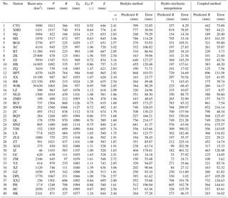
Our study area is in the upstream of the Bengbu Sluice in the HRB and is 121 000 km² (Fig. 1). The river network in the area is derived from data packages of the National Fundamental Geographic Information System, developed by the National Geomatics Center of China. The HRB is divided into 40 sub-basins, according to available hydrological stations with records from 1961 to 2000 (Fig. 2). The sub-basins vary in their size from the smallest of 17.9 km² to the largest of 30 630 km². Among the 40 sub-basins, 27 are independent sub-basins and 13 are nested sub-basins.

Figure 1 The topography and river network of the study area.

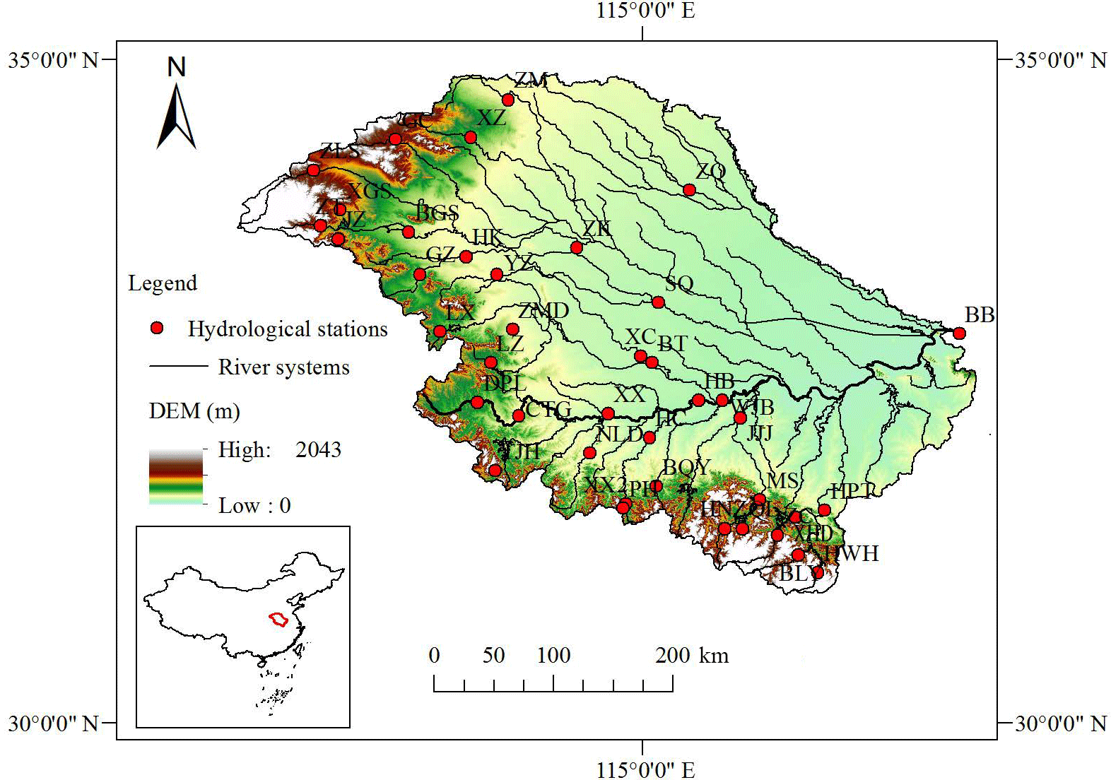
Annual precipitation data used in this study are from 1961 to 2000 and are obtained from a monthly mean climatological dataset at 0.5 ^∘ spatial resolution. The dataset was developed at the China Meteorological Administration, and is accessible at http://data.cma.cn/data/detail/dataCode/SURF_CLI_ CHN_PRE_MON_GRID_0.5.html (last access: 13 May 2018). The dataset was derived from the observations at 2472 stations in China, using the thin plate spline (TPS) interpolation method and the ANUSPLIN software. Pan evaporation data at 21 meteorological stations in the HRB are used to interpolate E₀ by the ordinary Kriging method and the ArcGIS. The interpolated E₀ are used to derive the annual potential evapotranspiration in the sub-basins. The statistical features of the mean annual precipitation (P), E₀, and the runoff depth (R) from 1961 to 2000 are summarized in Table 1. They show that P varied between 638 and 1629 mm, annual temperature was between 11 and 16 ^∘C, and the mean annual E₀ between 900 and 1200 mm. The sub-basins in the north, e.g., ZM, ZQ, XY, and ZK in Fig. 2, are relatively dry, with the dryness index (E₀∕P) above 1.3. The sub-basins in the south, e.g., MS, HBT, and HC, are wetter, with the dryness index below 0.8. The average mean annual R is about 400 mm, fluctuating from 90 mm in the north to 1000 mm in the south. The temporal and spatial variations in the runoff are relatively small in the south and large in the north.

Table 1 Summary of hydro-meteorological data and predicted runoff of the sub-basins in the HRB.

Figure 2 The sub-basins and hydrological stations in the study area.

4 Results

4.1 Prediction of runoff by the Budyko method

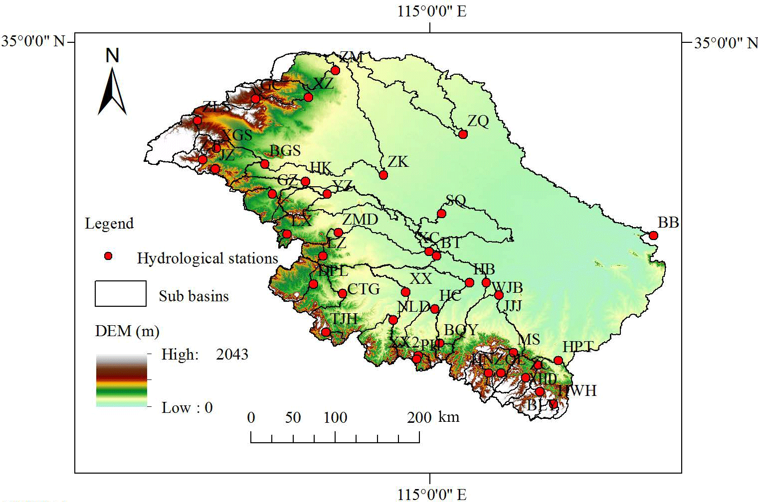
Actual evapotranspiration E is estimated using the long-term mean annual water balance ($E=P-R$) from 1961 to 2000 at the 40 sub-basins, and the results are shown in Table 1. Also shown in Table 1 are the calculated ω values for the sub-basins. They vary from 1.43 in the sub-basin HWH to 3.16 in JJJ. The average ω is 2.32 for the 40 sub-basins. The comparison E∕P vs. E₀∕P is shown in Fig. 3. The best fit (curve) for E∕P vs. E₀∕P, or R vs. $E_{\mathrm{0}}/P,$ is also shown in Fig. 3; it gives an alternative for average ω of the sub-basins. The fitted value of ω for the 40 sub-basins determined from this process is 2.213, very close to that calculated directly from the 40 individual sub-basins.

Using ω=2.213 in the HRB, Fu's equation in Eq. (2) can be written as

$$\begin{array}{}\text{(13)}& R=P{\left(\mathrm{1}+{\left({\displaystyle \frac{E_{\mathrm{0}}}{P}}\right)}^{\mathrm{2.213}}\right)}^{\frac{\mathrm{1}}{\mathrm{2.213}}}-E_{\mathrm{0}}.\end{array}$$

Equation (13) and Fig. 3 clearly show the deterministic trend of the runoff in the HRB. According to the water limit criterion, $E=P,$ and the energy limit criterion, E=E₀, in Fig. 3a, the smaller the index E₀∕P is, the smaller the E∕P will be (Fig. 3a) or the larger the runoff will be (Fig. 3b) from the sub-basins in the HRB. In Fig. 3b and c, the lower R in the northern sub-basins indicates drier conditions (E₀∕P > 1.4), whereas the higher R in the southern sub-basins ensures wetter conditions (E₀∕P < 0.8).

Figure 3 (a) E∕P ∼ E₀∕P and (b) R ∼ E₀∕P for the 40 sub-basins (the solid line is the best fit function). (c) The sub-basins in the north and south of the study basin. Note: in (b) and (c), blue color indicates wetter climate in the south and yellow color indicates drier climate in the north.

Using P and E₀ given in Table 1 for the 40 sub-basins, we predict the runoff R by Eq. (13), the Budyko method, and the deviations of their predictions from the observation. The results are summarized in Tables 1 and 2. The MAE of predicted R is 94 mm, and RMSE is 112 mm. The largest absolute error is in the sub-basin HWH (328 mm), and the smallest in XX (24 mm). The largest relative error is 81.6 % of the observed runoff in the sub-basin XZ, and the smallest is 5.0 % of the observed runoff in XHD. They represent absolute errors of 91 and 37 mm in those two sub-basins, respectively.

4.2 Runoff by the hydro-stochastic interpolation method

For comparison, the observed runoff is used in the hydro-stochastic interpolation following the procedure detailed in Sect. 2.2. In order to obtain the distance d between pairs of the sub-basins, the study area is divided into 40 rows × 50 columns. The geostatistical distance between any two sub-basins, A and B, is calculated by averaging the distances between all pairs of grid points in A and B (all the possible pairs of the sub-basins are 40 × 41∕2 for the 40 sub-basins in this study). According to the estimated distance for the pairs of sub-basins and the observed runoff at the 40 sub-basins (Table 1), the empirical covariance Cov_e(d) is estimated for each pair of the sub-basins. From the plots of the mean Cov_e(d) of all the independent sub-basin pairs vs. the corresponding distance d with an interval of 20 km, we fit the function of the empirical covariogram shown in Fig. 4. The fitting theoretical covariance function Cov_p(d) to the empirical covariogram is

$$\begin{array}{}\text{(14)}& {\mathrm{Cov}}_{\mathrm{p}}\left(d\right)=\mathrm{6}\times {\mathrm{10}}^{\mathrm{5}}\exp \left(-d/\mathrm{28.62}\right).\end{array}$$

This function is used to calculate the average theoretical covariance Cov(AB) in Eq. (7). Finally, the weight matrices are determined using our programs in MatLab.

Figure 4 Empirical covariogram (Cov_e(d)) from the sub-basin runoff data and theoretical covariogram by the fitted covariance function Cov_p(d) of the study area.

The interpolated runoff depth (R) over the 40 sub-basins along with the deviations from the observation are shown in Table 1. The MAE and RMSE of R are 103 and 140 mm, respectively. The largest absolute and relative error is in the sub-basin JZ (401 mm and 68.8 %), and the smallest is in DPL (1 mm and 0.3 %) (Table 2). These results indicate that the errors from this interpolation method are in general larger than those from the Budyko method, suggesting that the observed runoff is more influenced by the deterministic trend in the basin.

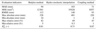
Table 2 Interpolation cross-validation errors between the predicted and observed runoff in the 40 sub-basins in the HRB from the three methods.

4.3 Hydro-stochastic interpolation with Fu's equation (our coupled method)

We use Fu's equation, Eq. (2), to evaluate the deterministic trend or the external drift function, $R_{\mathrm{d}}^{*}\left(x\right)$, and deviation of the trend from the observation, $R_{\mathrm{s}}^{*}\left(x\right)$, assuming a spatially auto-correlated process. The $R_{\mathrm{s}}^{*}\left(x\right)$ is then used in the stochastic interpolation.

The empirical residual covariogram of $R_{\mathrm{s}}^{*}(x$) for each pair of sub-basins vs. sub-basin distance is shown in Fig. 5. From the result in Fig.  5a, we obtain the exponential function for Cov_p(d):

$$\begin{array}{}\text{(15)}& {\mathrm{Cov}}_{\mathrm{p}}\left(d\right)=\mathrm{13}\mathrm{030}\exp \left(-d/\mathrm{23.9}\right).\end{array}$$

From Eq. (15), the weight matrices of runoff deviation are determined by Eq. (4) using our program in MatLab. They are then used to predict the runoff deviation. The scatterplot of the predicted residuals vs. the observed residuals shown in Fig. 5b delineates a positive correlation between the predicted and the observed residuals. However, the large scatter indicates limited performance by the residual model alone. Because this interpolation scheme represents the spatial runoff deviation, the sum of the interpolated runoff deviation and the simulated runoff by Fu's equation is the total interpolated runoff in the sub-basins.

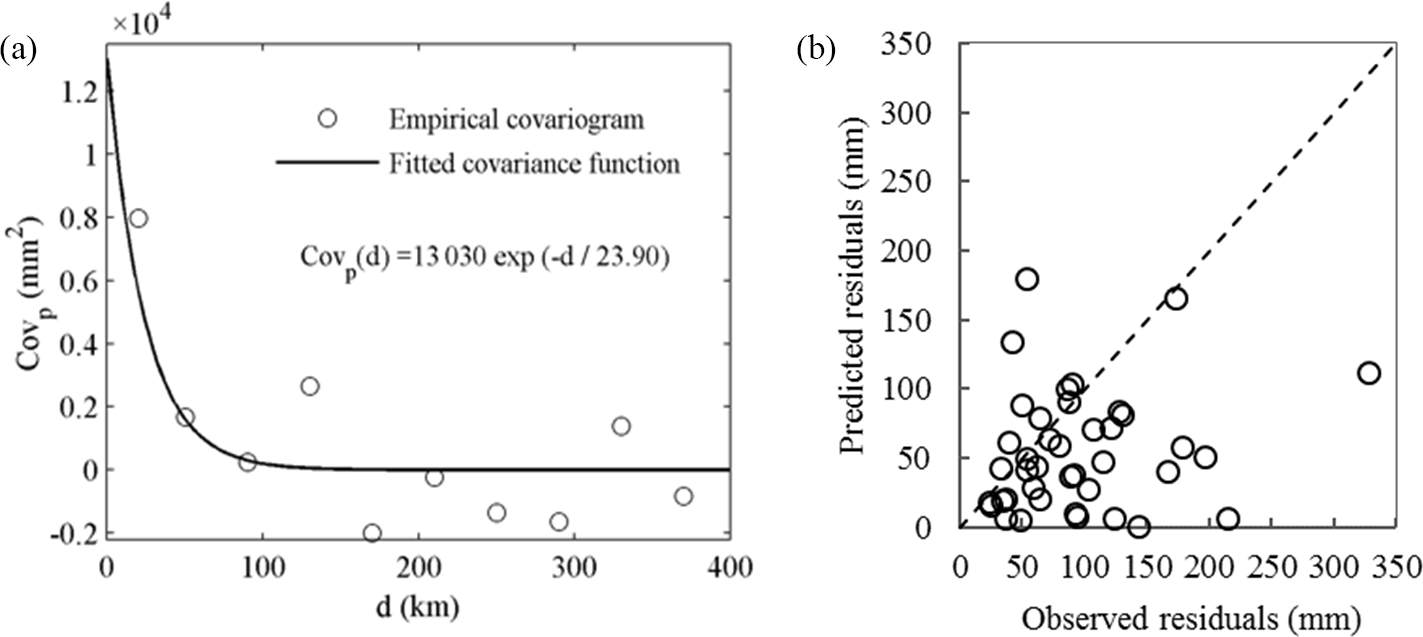
Figure 5 (a) Empirical covariogram (Cov_e(d)) from the residual R_s(x) and theoretical covariogram by the fitted covariance function Cov_p(d) of the study area. (b) The scatterplot of the predicted vs. observed residuals.

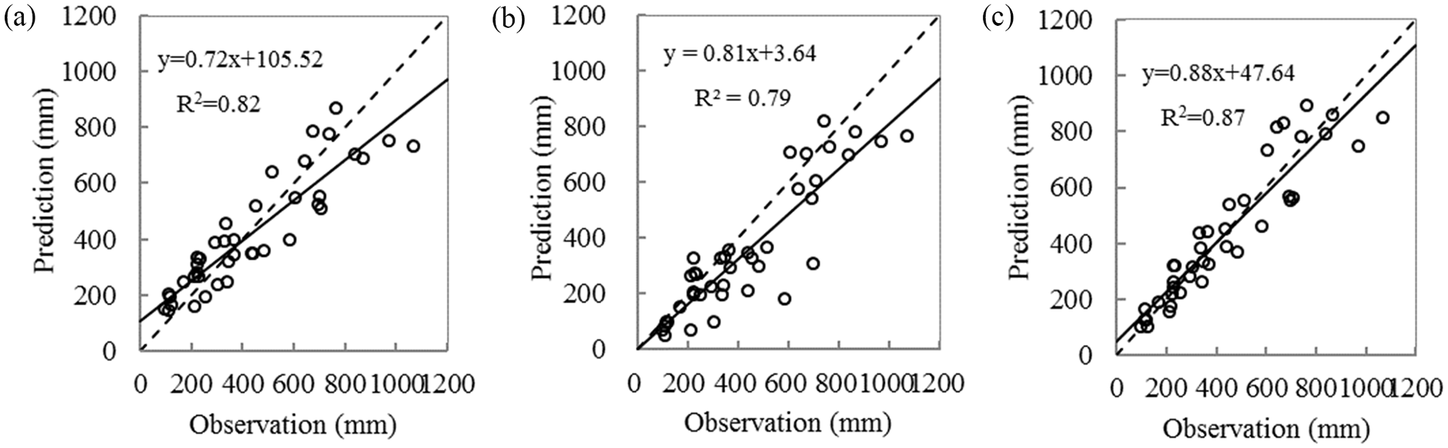
Figure 6 Cross-validation of the predicted runoff vs. the observation by (a) the Budyko method, (b) hydro-stochastic interpolation, and (c) our coupled method. The dashed line is 1 : 1.

The predicted runoff using this procedure is given in Table 1, with the MAE at 71 mm and RMSE at 93 mm over the 40 sub-basins. The largest absolute error is in the sub-basin QL (220 mm), and the smallest in ZM (4 mm) (Table 2). The largest relative error is 47.2 % of the observed runoff in XZ, and the smallest is 1 % of the observed runoff in BLY. They represent the absolute errors of 52 and 8 mm, respectively.

4.4 Comparisons of the predicted runoff by the three methods

Comparing the results in Table 2, we find that our coupled method of the deterministic and stochastic processes substantially reduces the runoff prediction error in the HRB. The MAE and RMSE of the runoff from our coupled method are much smaller than those from the Budyko or the hydro-stochastic interpolation method. In cross-validation (Table 2), our coupled method has $R_{\mathrm{cv}}^{\mathrm{2}}=$0.87, which is larger than 0.81 and 0.71 from the Budyko method and the hydro-stochastic interpolation, respectively. The errors in runoff at the sub-basins are significantly reduced as well. The error in the sub-basin HWH is 216 mm from the coupled method, compared to 328 mm from the Budyko method and 300 mm from the hydro-stochastic interpolation. The error in JZ is 120 mm from the coupled method, smaller than 179 mm from the Budyko method and 401 mm from the hydro-stochastic interpolation.

Our correlation analysis between the predicted and observed R is shown in Fig. 6. The predicted runoff from our coupled method shows higher correlation with the observed one (R²= 0.87), in comparison to the Budyko method (R²= 0.82) and the hydro-stochastic interpolation (R²= 0.79). Our analysis indicates that the latter two methods overestimate low runoff and underestimate high runoff, as indicated by large departures from the 1 : 1 line in Fig. 6. Similarly, large deviations of the runoff predicted by the hydro-stochastic interpolation have also been reported by Sauquet et al. (2000), Laaha and Blöschl (2006), and Yan et al. (2011).

The spatial distributions of the runoff in the HRB calculated from the three methods are shown in Fig. 7. They again show significant differences. Compared to the result from our coupled method (Fig. 7c), the Budyko method overestimates the runoff in most of the northern sub-basins (Fig. 7a), where the climate is relatively dry and runoff is small (ranging from 140 to 280 mm). The hydro-stochastic interpolation method underestimates the runoff in some southern sub-basins (Fig. 7b), where the wet climate has fostered extremely high runoff (800–1100 mm), such as in the sub-basins HWH, BLY, and ZC (Table 1). The results from our coupled method are closest to the observed distribution of the runoff among the three methods (Fig. 7d). Compared to the errors in the predicted runoff by the Budyko method and the hydro-stochastic interpolation (Fig. 7 and Table 1), our coupled method reduces the error in 70 % of all the sub-basins (28 of the 40 sub-basins).

Figure 7 Spatial distribution of the mean annual runoff estimated from (a) the Budyko method, (b) hydro-stochastic interpolation, (c) our coupled method, and (d) the observation.

5 Discussions and conclusions

In this study, we use the Budyko deterministic method to describe the mean annual runoff, which is an integrated spatially continuous process and determined by both the hydro-climatic elements and the hierarchical river network. A deviation from the Budyko estimated runoff is used by the stochastic interpolation that assumes spatially auto-correlated error. The deterministic aspects of the runoff described in the Budyko method are reflected in the trends at locations (sub-basins), and deviations from the trends caused by the stochastic processes are described by the weights as a function of the autocorrelation and distance. Information from both the Budyko method and the stochastic interpolation are integrated into our coupled method to predict the runoff.

Different from the universal Kriging method, in which the trend is represented as a linear function of coordinate variables and determined solely through spatial data calibration (i.e., semi-variogram analysis), the Budyko method couples water and energy balance and could directly predict streamflow in ungauged basins. This physically based method relies on using the spatial trend of runoff and, in our study, it yields the deterministic coefficient of cross-validation, $R_{\mathrm{cv}}^{\mathrm{2}}$, to be 0.81, better than that from the hydro-stochastic interpolation method.

Incorporating secondary information into the geostatistical methods improves the estimate of a predictive variable, e.g., the estimate of groundwater level by incorporating topography into the collocated co-Kriging (Boezio et al., 2006), or the estimate of mean annual stream temperature by incorporating a nonlinear relationship between the mean annual stream temperature and altitude of the stream gauge into the top Kriging (Laaha et al., 2013). By incorporating such secondary information and the relationship between the mean runoff and the climate conditions (the aridity index) into the Budyko method through coupling with the hydro-stochastic interpolation, we develop our new coupled Budyko–hydro-stochastic interpolation method. It can substantially improve the prediction of streamflow in ungauged basins. This improvement is shown by the higher $R_{\mathrm{cv}}^{\mathrm{2}}$ of 0.87 in the HRB, compared to 0.81 and 0.71 by the Budyko and hydro-stochastic interpolation methods, respectively. Moreover, for high and low runoffs in the sub-basins of the HRB, our coupled method gives more accurate predictions.

While substantial progress has been made by our coupled method, its results show room for improvement to further increase the accuracy of runoff prediction. For example, runoff prediction errors remain large from our coupled method in some sub-basins in the HRB. In the sub-basins MS, QL, HWH, and HNZ, the absolute error of predicted runoff is larger than 150 mm and the relative error of predicted runoff is larger than 20 % of the observed runoff. In the sub-basins BGS and XZ, the relative error of the predicted runoff is larger than 40 % of the observed runoff. These errors are largely attributable to large prediction errors intrinsic to the Budyko method (e.g., MS, QL, HWH, and XZ in Table 1). Possible causes of the errors could be from additional external factors influencing the runoff, such as land cover, soil properties, hydro-climatic variations, and the groundwater. Including some or all of these effects to improve the Budyko method or incorporating these effects as secondary information (e.g., multi-collocated co-Kriging) into our coupled model would help aid our understanding of the deterministic processes and increase the runoff prediction accuracy.