Obtaining sub-daily new snow density from automated measurements in high mountain regions

The density of new snow is operationally monitored by meteorological or hydrological services at daily time intervals, or occasionally measured in local field studies. However, meteorological conditions and thus settling of the freshly deposited snow rapidly alter the new snow density until measurement. Physically based snow models and nowcasting applications make use of hourly weather data to determine the water equivalent of the snowfall and snow depth. In previous studies, a number of empirical parameterizations were developed to approximate the new snow density by meteorological parameters. These parameterizations are largely based on new snow measurements derived from local in situ measurements. In this study a data set of automated snow measurements at four stations located in the European Alps is analysed for several winter seasons. Hourly new snow densities are calculated from the height of new snow and the water equivalent of snowfall. Considering the settling of the new snow and the old snowpack, the average hourly new snow density is 68 kg m⁻³, with a standard deviation of 9 kg m⁻³. Seven existing parameterizations for estimating new snow densities were tested against these data, and most calculations overestimate the hourly automated measurements. Two of the tested parameterizations were capable of simulating low new snow densities observed at sheltered inner-alpine stations. The observed variability in new snow density from the automated measurements could not be described with satisfactory statistical significance by any of the investigated parameterizations. Applying simple linear regressions between new snow density and wet bulb temperature based on the measurements' data resulted in significant relationships (r² > 0.5 and p ≤ 0.05) for single periods at individual stations only. Higher new snow density was calculated for the highest elevated and most wind-exposed station location. Whereas snow measurements using ultrasonic devices and snow pillows are appropriate for calculating station mean new snow densities, we recommend instruments with higher accuracy e.g. optical devices for more reliable investigations of the variability of new snow densities at sub-daily intervals.

1 Introduction

In mountain regions there is an increasing demand for high-quality analysis, nowcasting and short-range forecasts of the spatial distribution of snowfall. Operational services, concerning avalanche warning, road maintenance and hydrology, as well as hydropower companies and ski resorts, need reliable information on the depth of new snow (HN) and the water equivalent (HNW) of snowfall. Therefore the new snow density (ρ_HN) is needed to convert HN into HNW and vice versa. Information on HN is especially relevant for cold and windy conditions, when measuring HNW is a difficult task because conventional rain gauge measurements are prone to large errors (e.g. Goodison et al., 1998). Recent results of the Solid Precipitation Intercomparison Experiment (SPICE; Nitu et al., 2012) reveal that these errors still exist in standard meteorological measurements (e.g. Buisán et al., 2016; Pan et al., 2016). Many snow cover models calculate HN from HNW at sub-daily time intervals, although reliable HNW input data are difficult to obtain (Egli et al., 2009), and thus the new snow density is needed in equal temporal resolution to convert between HNW and HN (e.g. Lehning et al., 2002; Roebber et al., 2003; Olefs et al., 2013). Additionally, ρ_HN has a considerable effect on the snow bulk density of the total snowpack (e.g. Schöber et al., 2016).

Since the 1960s ultrasonic rangers have become more common for observing snow depth changes automatically even at sub-hourly time intervals (e.g. Gubler, 1981; Goodison et al., 1984; Lundberg et al., 2010). They have the advantage of a more objective method compared to subjective manual measurements of snow depth (Ryan et al., 2008). Although high-accuracy optical snow depth sensors have been more frequently used in practice over recent years (e.g. Mair and Baumgartner, 2010; Helfricht et al., 2016), longer time series of snow depths exist from ultrasonic measurements. Beside snow depth (HS), the water equivalent of the snowpack (SWE) is observed operationally using weighing devices such as lysimetric snow pillows (e.g. Serreze et al., 1999; Egli et al., 2009; Lundberg et al., 2010; Krajči et al., 2017) and snow scales (e.g. http://www.sommer.at/en/products/snow-ice/snow-scales-ssg-2, last access: 3 May 2018). Upward-looking GPR (e.g. Heilig et al., 2009) and GPS techniques (e.g. Koch et al., 2014; McCreight et al., 2014) and the combination of both (Schmid et al., 2015) have been applied in scientific studies to monitor the depth, SWE and liquid water content of the snowpack. However, these techniques are rather expensive or not yet in use for long-term observations by operational services. In general, automatic measurements of SWE are prone to a high relative uncertainty and require a certain degree of maintenance, which makes them complex and labour-intensive (Smith et al., 2017). Due to such constraints, SWE measurement instrumentation is installed at considerably fewer stations compared to HS instruments, and only at sites with easy access for appropriate maintenance. Recent studies present the performance of cosmic ray neutron sensors (e.g. Schattan et al., 2017), which are partly used for long-term observations such as e.g. from Col de Porte (Morin et al., 2012).

The density of new snow is influenced by the shape and size of the snow crystals (e.g. Nakaya, 1951). Relationships between predominant snow crystal type, riming properties and snowfall density were already reported by Power et al. (1964) from snowstorm observations in Canada. Once the snow crystals have accumulated at the snow surface, the density of the fresh snow starts to increase depending on prevailing weather conditions and compaction caused by overlaying of snow. A common mean ρ_HN used to convert between HN and HNW is 100 kg m⁻³. Many studies analysed ρ_HN values on a daily basis and confirmed this 10 : 1 rule as applicable for a first estimate (e.g. Roebber et al., 2003; Egli et al., 2009; Teutsch, 2009). However, ρ_HN values span a wide range, and values from 10 to 350 kg m⁻³ have been reported from American and European mountain ranges, with mean values between 70 and 110 kg m⁻³ (e.g. Diamond and Lowry, 1954; LaChapelle, 1962; Power et al., 1964; Judson, 1965; McKay et al., 1981; Meister, 1985; Judson and Doesken, 2000; Valt et al., 2014). Most of the ρ_HN data analysed in these studies were observed using readings on a snow board. The density is calculated from HN measured with a ruler and HNW is derived from an external precipitation device or from weighing the new snow either in solid or melted form (Fierz et al., 2009).

Several studies have shown that measured ρ_HN can be related to meteorological parameters, although with different time intervals and different degrees of determination. Gold and Power (1952) showed that the crystal type is related to its estimated formation temperature. Diamond and Lowry (1954) and Simeral et al. (2005) built an empirical calculation that ascertained relationships between ρ_HN and air temperature at the 700 mb level. Teutsch (2009) also concluded that ρ_HN of 12 h intervals at valley stations is best correlated to the wet bulb temperature at mountain stations in close vicinity (r² = 0.86). Judson and Doesken (2000) found that near-surface air temperature and new snow density at mountain stations could explain 52 % of the variance in snow density. Wetzel et al. (2004) presented a similar degree of correlation of ρ_HN to temperature at three high-elevation sites. Alcott and Steenburg (2010) showed that ρ_HN is correlated with near-crest-level temperature and wind speed particularly for high-SWE events. Wright et al. (2016) presented a statistical analysis of data from 42 seasons of manual daily snow density measurements along with air temperature and wind speed to derive parameterizations to estimate new snow density. However, they end up with a low coefficient of determination.

On the basis of data from seven stations in Switzerland located between 1250 and 1800 m a.s.l., Meister (1985) concluded that ρ_HN does not correlate with the amount of new snow (HN), that it does not depend on altitude and that air temperature does not accurately determine ρ_HN. Nevertheless, binning the data into temperature classes results in a statistical equation with a correlation coefficient of 0.85. Further, he recommended considering wind speed in addition to air temperature, at least for stations higher than 1800 m a.s.l. On the basis of data sets from Schmidt and Gluns (1991) and the US Army Corps of Engineers (1956), Hedstrom and Pomeroy (1998) developed a power function using the air temperature, for which they found a coefficient of determination of 0.84 and a standard error of estimate of 9.3 kg m⁻³. Jordan et al. (1999) introduced an algorithm for assigning ρ_HN within the SNTHERM snow cover model. They added wind dependence to the temperature parameterization of Meister (1985). This achieved a reduction of the error, but a significant scatter remained between observed and parameterized ρ_HN values. Lehning et al. (2002) built an empirical calculation for ρ_HN valid for a time interval of 30 to 60 min in the framework of the snow model SNOWPACK. They used air temperature, surface temperature, relative humidity and wind speed for the regression analysis and achieved an approximate multiple coefficient of determination of 0.83. Schmucki et al. (2014) used another empirical power relation, including air temperature, wind speed and relative humidity, to calculate the ρ_HN using SNOWPACK simulations for three contrasting sites in Switzerland. ρ_HN was analysed in short time intervals of 1–2 h by Ishizaka et al. (2016). They measured even lower densities in comparison to ρ_HN estimates obtained using the SNOWPACK density model, especially for aggregated snow crystal types. On the basis of data from Col de Porte (1325 m altitude, French Alps), Pahaut et al. (1976) developed a statistical relationship including the melting point of water, air temperature and wind speed. This parameterization is used to calculate the density of new snow in the snow cover model CROCUS (Vionnet et al., 2012).

Settling of the new snow by its weight and destructive metamorphism may reduce HN and hence increase ρ_HN between snowfall and the HN reading and has to be considered when computing new snow density (e.g. Anderson, 1976; Lehning et al., 2002; Steinkogler, 2009; Vionnet et al., 2012). The contribution of settling to snow depth changes is highest in the first hours after snowfall. Wind drift and radiation input to the snow surface after the snowfall may increase ρ_HN in comparison to ρ_HN at the time of snowfall. However, direct measurements of ρ_HN at the time of snowfall are laborious and difficult to align with the hours of peak snowfall rates.

Whereas most of the studies have analysed daily and sub-daily, manual ρ_HN measurements, to the best of our knowledge no extensive analysis of automated ρ_HN measurements in hourly intervals over several winter seasons exists. The aim of this study is to assess the value of automated measurements of hourly HN and HNW for the calculation of ρ_HN at different stations and at hourly time intervals. Therefore we examine the following questions.

1. Are automated measurements of HN and HNW suitable for the calculation of ρ_HN at hourly intervals?

2. How do the mean and the variability of observed ρ_HN differ between distinct study sites?

3. How well do established density parameterizations represent observed hourly ρ_HN values?

To this end, we calculated ρ_HN from hourly snow depth changes (HN) and hourly SWE changes (HNW). The mean values and the variability of hourly ρ_HN are discussed for observations at four different meteorological stations and compared to calculations using established ρ_HN parameterizations. A critical assessment with an outlook for next-generation measurement techniques is given in the discussion.

2 Data and methods

Data from four automatic weather stations (AWSs) were used in this study (Fig. 1, Table 1). A prerequisite for the station selection was the combined measurement of HS and SWE at each station in addition to the standard meteorological measurements of air temperature, relative humidity, precipitation, wind speed and global radiation. HS data are measured using ultrasonic rangers. SWE data are recorded using snow pillows. Details regarding the instruments at each AMS and the exact location of each AWS, as well as the start and end dates of the available data coverage, are presented in Table 1.

Figure 1 Map of the station locations. Pictures are given for (a) Weissfluhjoch station, (b) Kühtai station, (c) Wattener Lizum station and (d) Kühroint station.

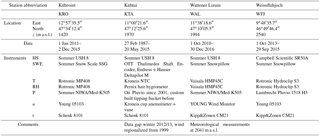
Table 1 Coordinates and data availability are given for the four snow stations. The instrumentation for measuring snow depth (HS), snow water equivalent (SWE), temperature (T), relative humidity (RH), precipitation (P), wind speed (u) and global radiation (r) is listed.

The Kühroint station (Germany) is operated by the Bavarian Avalanche Warning Service. It is a well-equipped and maintained station for snow climate at the northern fringe of the eastern Alps. It is located in a meadow below the tree line.

The Kühtai station (Austria) is operated by the Tiroler Wasserkraft AG (TIWAG). It is located south of the Inntal valley, but north of the Alpine main ridge, and it is situated in a wind-sheltered location.

The station at Wattener Lizum (Austria) is operated by the Austrian Research Centre for Forests (BFW) of the Federal Ministry of Agriculture, Forestry, Environment and Water Management. This station is situated in a south–north-oriented high alpine valley above the tree line near to the Alpine main ridge. This station has an exceptionally long time series of snow-hydrological measurements (Krajči et al., 2017; Parajka, 2017).

The station at Weissfluhjoch (Switzerland) is operated by the Institute for Snow and Avalanche Research (SLF), which is part of the Swiss Federal Institute for Forest, Snow and Landscape Research (WSL). The station is presented in more detail by Marty and Meister (2012). Weissfluhjoch is the highest elevated station considered in this study.

On the basis of coinciding data availability we consider four time periods as presented in Table 1. Data outputs of the AWSs are logged at time intervals ranging from 2 to 30 min. Hourly values were computed for global radiation, relative humidity, air temperature and wind speed. The hourly value is the mean of the previous hour. For precipitation it is the sum of the previous hour. To account for noise in the ultrasonic signal, HS and SWE were smoothed using a centred moving average over three values in the original data resolution. The hourly values for HS and SWE are the values from the smoothed time series.

The thermodynamic wet bulb temperature (T_w) was computed applying the psychrometric equation (Sonntag, 1990) and an exact iterative approach presented by Olefs et al. (2010). A standard barometric equation was used to determine air pressure based on the station elevation. Air pressure dependency of T_w is generally minor and only relevant for air temperatures larger than +2 ^∘C (Olefs et al., 2010).

A necessary condition for all further analysis of the time series was the presence of a precipitation signal at the heated precipitation gauges in combination with positive snow depth changes. Then, the hourly height of new snow (HN) and the water equivalent of snowfall (HNW) were computed as the change in HS and SWE. Within the next filtering step, only HN and HNW values with T_w less than 0 ^∘C and a wind speed (u) of less than 5 m s⁻¹ were considered.

Constraints have to be set in order to avoid low values of HNW and HN, which are prone to large relative errors due to random and systemic measurement uncertainties in HN and SWE, but a minimum of approx. 100 remaining samples for statistical analysis must be ensured.

To investigate the influence of different minimum HNW and HN limits, a distribution matrix was calculated by varying the minimum HNW and HN limits in steps of 0.5 mm for HNW and 0.5 cm for HN, respectively. To account for settling during ongoing snowfall, the compaction correction described in Anderson (1976) was applied. The approach was simplified with respect to HS, SWE and snow density by considering only two layers of the snowpack: the new snow and the total snowpack of the previous time step. Destructive settling (S) of HN is considered for each time step in which the snow depth increases (Eq. 1). The destructive settling of the new snow (S_HN) for each time step is calculated by

$$\begin{array}{}\text{(1a)}& {\displaystyle }& {\displaystyle }{S}_{\mathrm{HN}}=-\mathrm{0.000002777}\cdot e^{\left(\mathrm{0.04}\cdot T\right)}\left\{{\mathit{\rho }}_{\mathrm{HN}}\le \mathrm{150}\mathrm{kg}{\mathrm{m}}^{-\mathrm{3}}\right\}\text{(1b)}& {\displaystyle }& {\displaystyle }{S}_{\mathrm{HN}}=S_{\mathrm{HN}}\cdot e^{\left(\mathrm{0.046}\cdot T\cdot ({\mathit{\rho }}_{\mathrm{HN}}-\mathrm{150})\right)}\left\{{\mathit{\rho }}_{\mathrm{HN}}\ge \mathrm{150}\mathrm{kg}{\mathrm{m}}^{-\mathrm{3}}\right\},\end{array}$$

where T is the air temperature. Settling of the new snow layer caused by the weight of the ongoing snow accumulation is not taken into account.

Settling within the old snowpack is computed considering the total snow depth (HS). The destructive settling within the old snow layer (S_HS) is calculated using Eq. (1), substituting HS for HN and using the bulk density of the old snowpack (ρ_HS) calculated from HS and total SWE of the previous time step. Settling within the old snowpack caused by the weight of the snowpack (S_wHS) is given as

$$\begin{array}{}\text{(2)}& S_{\mathrm{wHS}}=-\mathrm{248.976}\cdot {\displaystyle \frac{\mathrm{HN}}{\mathrm{3}\mathrm{600}\mathrm{000}}}\cdot e^{\mathrm{0.8}\cdot T}\cdot e^{-\mathrm{0.021}\cdot {\mathit{\rho }}_{\mathrm{HS}}}.\end{array}$$

The resulting settling factors of S_HN, S_HS and S_wHS are multiplied by HS and HN to adjust HN accordingly.

New snow density (ρ_HN) was obtained from the ratio of HN to HNW. Outliers below the 5 % percentile and higher than the 95 % percentile were excluded. The ρ_HN data were grouped by wet bulb temperature and wind speed, using bins of 1 ^∘C and 0.5 ms⁻¹ respectively. A least squares regression was carried out using both the ungrouped data and the median of the grouped data to quantify possible correlations of ρ_HN with T_w and u.

The ρ_HN values were compared to the following parameterizations developed in previous studies. In these parameterizations, ρ_HN is a function of meteorological parameters such as air temperature (T), wind speed (u) and relative humidity (RH). The time interval for ρ_HN readings of the respective study is given in brackets.

$$\begin{array}{ll}{\displaystyle }& {\displaystyle }{\mathit{\rho }}_{\mathrm{HP}}=\mathrm{67.92}+\mathrm{51.52}\cdot e^{\frac{T}{\mathrm{2.59}}}\text{(Hedstrom and Pomeroy 1998,}\\ \text{(3)}& {\displaystyle }& {\displaystyle }\text{event/daily)}{\displaystyle }& {\displaystyle }{\mathit{\rho }}_{\mathrm{D}}=\mathrm{119}+\mathrm{6.48}T\text{(Diamond and Lowry 1954,}\\ \text{(4)}& {\displaystyle }& {\displaystyle }\text{frequent interval during event)}\text{(5)}& {\displaystyle }& {\displaystyle }{\mathit{\rho }}_{\mathrm{LC}}=\mathrm{50}+\mathrm{1.7}\cdot (T+\mathrm{15}{)}^{\mathrm{1.5}}\text{(LaChapelle 1962, event)}{\displaystyle }& {\displaystyle }{\mathit{\rho }}_J=\mathrm{500}\cdot \left(\mathrm{1}-\mathrm{0.951}\cdot {\mathrm{e}}^{-\mathrm{1.4}\cdot {\left(\mathrm{5}-T\right)}^{-\mathrm{1.15}}-\mathrm{0.008}{u}^{\mathrm{1.7}}}\right)\\ \text{(6a)}& {\displaystyle }& {\displaystyle }\left\{-\mathrm{13}{}^{\circ }\mathrm{C}<T\le \mathrm{2.5}{}^{\circ }\mathrm{C}\right\}{\displaystyle }& {\displaystyle }{\mathit{\rho }}_J=\mathrm{500}\cdot \left(\mathrm{1}-\mathrm{0.904}\cdot e^{-\mathrm{0.008}{u}^{\mathrm{1.7}}}\right)\left\{T\le \mathrm{13}{}^{\circ }\mathrm{C}\right\}\\ \text{(6b)}& {\displaystyle }& {\displaystyle }\text{(Jordan et al., 1999, event/daily)}{\displaystyle }& {\displaystyle }{\mathit{\rho }}_V=\mathrm{109}+\mathrm{6}\cdot \left(T-T_f\right)+\mathrm{26}{u}^{\mathrm{0.5}}\\ \text{(7)}& {\displaystyle }& {\displaystyle }\text{(Vionnet et al., 2012, event/daily}){\displaystyle }& {\displaystyle }{\mathit{\rho }}_S={\mathrm{10}}^{\mathrm{3.28}+\mathrm{0.03}T-\mathrm{0.36}-\mathrm{0.75}\cdot \arcsin (\sqrt{\mathrm{0.01}\mathrm{RH}}+\mathrm{0.03}\cdot {\log }_{\mathrm{10}}u)}\\ \text{(8a)}& {\displaystyle }& {\displaystyle }\left\{T\ge -\mathrm{14}{}^{\circ }\mathrm{C}\right\}{\displaystyle }& {\displaystyle }{\mathit{\rho }}_S={\mathrm{10}}^{\mathrm{3.28}+\mathrm{0.03}T-\mathrm{0.75}\cdot \arcsin (\sqrt{\mathrm{0.01}\mathrm{RH}}+\mathrm{0.03}\cdot {\log }_{\mathrm{10}}u)}\\ \text{(8b)}& {\displaystyle }& {\displaystyle }\left\{T<-\mathrm{14}{}^{\circ }\mathrm{C}\right\}\text{(Schmucki et al., 2014, event/hourly)}{\displaystyle }& {\displaystyle }{\mathit{\rho }}_{\mathrm{L}}=\mathrm{70}+\mathrm{6.5}T+\mathrm{7.5}{T}_{\mathrm{s}}+\mathrm{0.26}\mathrm{RH}+\mathrm{13}u-\mathrm{4.5}T{T}_{\mathrm{s}}\\ {\displaystyle }& {\displaystyle }-\mathrm{0.65}Tu-\mathrm{0.17}\mathrm{RH}u+\mathrm{0.06}T{T}_{\mathrm{s}}\mathrm{RH}\\ \text{(9)}& {\displaystyle }& {\displaystyle }\left(\text{Lehning et al., 2002, event/hourly}\right)\end{array}$$

The melting point of snow (T_f) in Eq. (7) was approximated as 0 ^∘C (Vionnet et al., 2012). Following Schmucki et al. (2014), we limited the parameter range and set RH to a constant value of 0.8 (80 %) during snowfall and the lower boundary for the wind speed to 2 ms⁻¹.

The temperature of the snow surface (T_s) is required in Eq. (9). As this was not available for each station, we used the approximation T_s= T. We argue that T_s could not considerably exceed 0^∘ because of the maximum T_w of 0 ^∘C. Since only precipitation events are considered, RH can be expected to be high, and thus the difference between T_w and T is small.

The uncertainty of ultrasonic measurements on snow can be assumed to be in the range of ±1 cm, which is partly a consequence of changes in signal velocity due to meteorological conditions. However, we used the original HS data logged in millimetre resolution to avoid the effects caused by rounding to full centimetre when calculating HN. Likewise, we used the tenths of millimetre SWE data logged at the pillows. Another documented error source of the HS measurement is signal blocking by e.g. dense snowfall or drifting snow, which causes peaks of the HS. However, with the filtering procedure applied in this study, no such spikes were left in the analysis.

A source of uncertainty is the spatial offset between the HS measurements and the SWE measurements. HS is measured directly above the SWE measurement at Kühtai station, Kühroint station and Wattener Lizum station (Fig. 1). However, the footprint of the snow depth sensor may be smaller than the surface area of the pillow, and it decreases with increasing HS. A spatial variability of HS on the pillow can be caused by snow drift and differing snow settling or snowmelt.

For the calculations within this study we used the changes in HS and SWE over the time period of snowfall only. Errors due to spatial variability in HS and SWE caused by spatial differences in energy consumption and snow drift between precipitation events are reduced. This is especially valid for the HS and SWE measurements at the stations with matching HS and SWE measurements. The snow depth sensor and the snow pillow of Weissfluhjoch station are separated by 9 m. Schmid et al. (2014) suggest a small-scale variability in HS of ±4.3 % at the Weissfluhjoch station. Again, the error may be smaller due to using temporally limited changes of HS, but an additional uncertainty of ±5 % can be assumed here.

A well-known issue with snow pillows is bridging effects (e.g. Serreze et al., 1999; Johnson and Schaefer, 2002). Dense snow layers and crusts within the snowpack sustain the weight of the new snow so that HNW, and thus ρ_HN, are underestimated. We cannot exclude such data explicitly. However, all filtering conditions have to be fulfilled to include values in the analysis, so that data without or with lagged HN increase were not considered. Additionally, the chosen snow stations are well maintained in case of implausible data due to their overall good accessibility; e.g. trenches are dug out around the base area of the snow pillow at Kühtai station to cut off the measured part of the snowpack to avoid bridging effects.

Nevertheless, the measurement uncertainty is ±1 cm for HN and 0.1 cm for HNW. Considering mean HN (Table 2) and HNW values, the uncertainty is ±25 kg m⁻³ or 37 % of the mean density. This value is lower considering higher HN, but increases to 80 % for the combination of minimum HN and minimum HNW of 1.6 and 0.2 mm respectively.

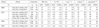
Table 2 Time periods analysed in this study with the mean and the median of hourly values for the height of new snow (HN), wet bulb temperature (T_w), wind speed (u), calculated densities from observed values (ρ) and calculated densities corrected for settling of the snowpack (ρ_HN). The results are valid for the filtered data values (n_th) with HN > 2 cm, HNW > 1.5 mm, T_w < 0 ^∘C and u < 5 ms⁻¹ as a subset of all data that have a precipitation signal and positive HS change (n_P).

3 Results and discussion

3.1 Data filtering, correction of settling and evaluation

Figure 2 presents the median new snow density (ρ_HN) data calculated from all filtered HN and HNW values exceeding the respective minimum HN and HNW limits. This presentation highlights the variability of ρ_HN by using different minimum limits with respect to the high relative uncertainty of low HN and HNW values. Changing the minimum limits for HN and HNW affects the resulting ρ_HN considerably. However, increasing the minimum limits for HN and HNW results in a distinct lowering of the number of data remaining for the subsequent analysis (Fig. 2). There are certain differences between the stations for high minimum HNW limits. Calculated ρ_HN decrease when low minimum HN and high minimum HNW limits are applied at Kühtai and Wattener Lizum station. In contrast, ρ_HN values increase for equal minimum limits at Kühroint and Weissfluhjoch stations. At Kühtai and Wattener Lizum stations, high HNW values of more than 3 mm HNW are accompanied by a rather high HN (Fig. 2). In contrast, a low HN occurring with a high HNW at Kühroint and Weissfluhjoch causes a high ρ_HN. However, these results are based on a small number of values only. In general, the calculated median ρ_HN values are rather constant following the 1 : 1 line of minimum HNW and HN limits (Fig. 2).

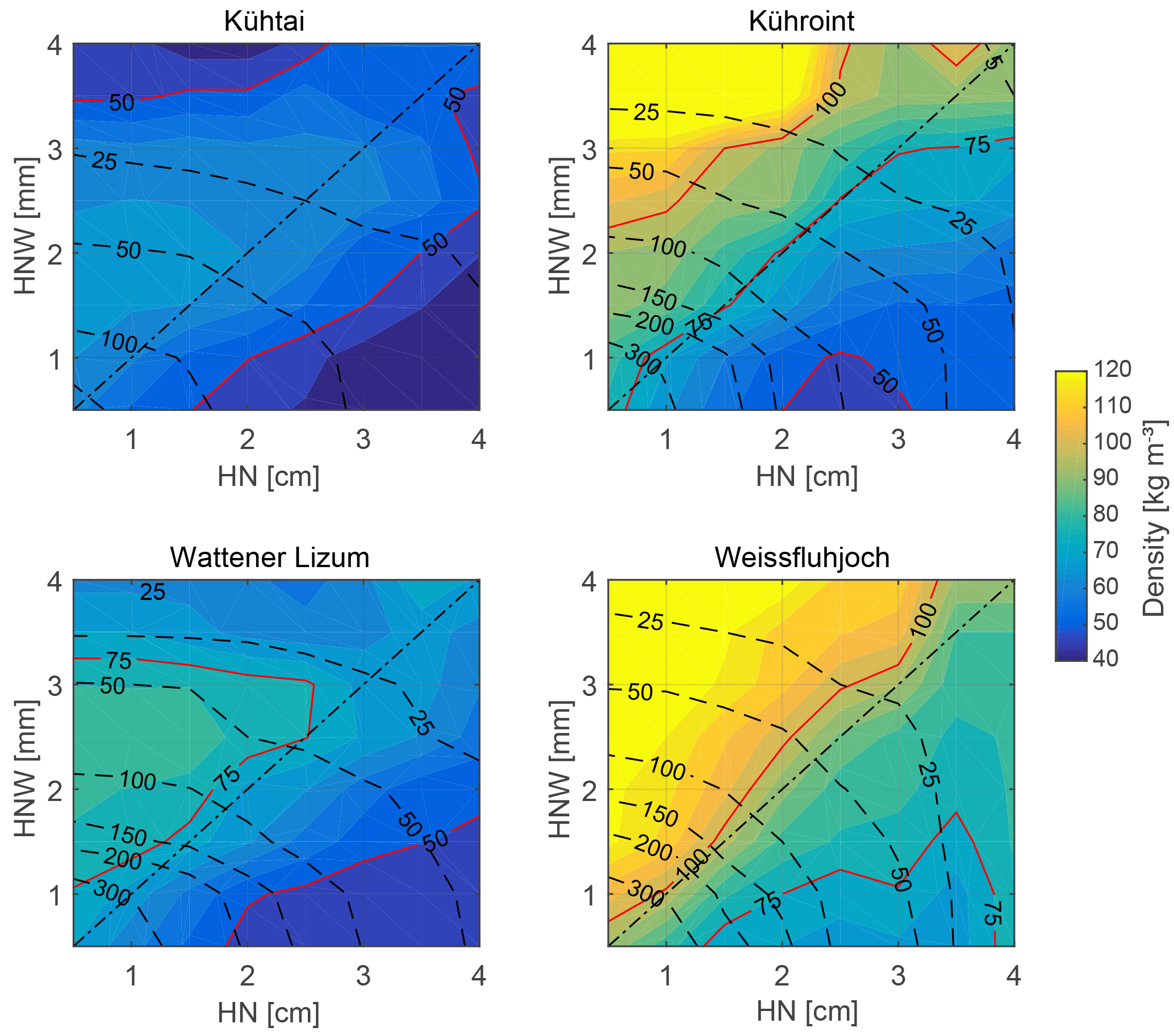
Figure 2 Median new snow densities (colour scale) calculated using all data exceeding different minimum limits of the height of new snow (HN) and the water equivalent of snowfall (HNW) for period 1 (1 October 2013–20 May 2015). Note that multiples of 25 kg m⁻³ are highlighted with red contour lines. The labelled black dashed lines give the count of the hourly data remaining after filtering. The straight dotted and dashed lines show results for equal minimum limits of HN (cm) and HNW (mm).

In order to avoid low values of HNW and HN, but ensuring an appropriate number of approx. 100 samples and with respect to the results of the Fig. 2, we decided to use a minimum limit of 1.5 mm in HNW and 2.0 cm in HN. This leads to the exclusion of on average 94 % of all data points that have a precipitation signal and positive snow depth changes (Table 2). Frequency distributions for HN, HNW, T_w and u of the unfiltered and filtered data are presented for each station and for each time period in the Supplement Figs. S01 to S09.

The exclusion of high wind speeds only has a small effect at the lower stations and is more noticeable at the more wind-exposed stations of Wattener Lizum and Weissfluhjoch. Considering period 1 comprising all stations, the filtering process causes the highest filtering rate for Weissfluhjoch station, with 6 % of data remaining after applying the filtering. The overall highest amount of data reduction is found at Kühtai station, with 5 % of the data remaining after filtering of the longer periods 3 and 4 (Table 2). There was a considerable fraction of data with positive HS changes, a precipitation signal and positive T_w. Most of these data seem to be paired with very small HS changes and are eliminated for the final data set when the HN minimum limit is applied.

The correction of the HN underestimation caused by settling of the snowpack during snowfall leads to an average reduction of mean ρ_HN of 10.2 kg m⁻³, with a standard deviation (σ) of 2.6 kg m⁻³ (Table 2). This corresponds to 13.5 % with a σ of 3.7 %. The compaction correction causes noticeably less change in ρ_HN at Weissfluhjoch in period 1 (5 % reduction of mean ρ_HN) than in the other time periods and other stations. The next closest is Kühroint, also in period 1, with a reduction in ρ_HN of 7 %. Unless otherwise stated in the text, ρ_HN always refers to the corrected densities hereafter. Based on a 15-year data set of Weissfluhjoch (WSL Institute for Snow and Avalanche Research SLF, 2015, https://doi.org/10.16904/1) from 1 September 1999 to 31 December 2015, the contribution of settling relative to HN was calculated using the multi-layer SNOWPACK model (e.g. Lehning et al., 2002) and the approach from Anderson (1976) to compare the results of this study to a more physically based estimate. Results are presented in Fig. 3. While a median relative contribution of settling to HN by 19 % was calculated with SNOWPACK, the approach of Anderson (1976) resulted in lower values of 5 % in median and 9 % in mean. Thus, the settling considered for the presented data can be assumed to be a lower estimation. However, higher contributions of settling would result in lower ρ_HN values, with an increased HN assuming a fixed HNW.

Figure 3 Box plots (median, 25 and 75 % percentiles, 1.5 × interquartile ranges, outliers) of settling relative to hourly new snow heights (HN) modelled with SNOWPACK and using the approach presented by Anderson (1976).

Figure 4 shows the distribution of ρ_HN values obtained from the filtered data at Kühroint station as representative of all stations and periods (Figs. S10 to S17). In general, the ρ_HN values show high variability at all stations. Nevertheless, ρ_HN values are within a reasonable range of less than 200 kg m⁻³. The histograms of ρ_HN show one-tailed distribution towards higher ρ_HN. Median ρ_HN values of the different stations and for different periods range between 66 and 86 kg m⁻³for uncorrected values and between 54 and 83 kg m⁻³ for ρ_HN corrected for settling (Table 2).

Figure 4 Distribution of calculated new snow densities at Kühroint station for period 1 (1 October 2013–20 May 2015). (a) All data have a precipitation signal and positive HS change, all data are filtered with HN > 2 cm, HNW > 1.5 mm, T_w < 0 ^∘C and u < 5 ms⁻¹) and filtered data are reduced by cutting off at 5 and 95 % percentiles. (b) Histogram of all filtered densities. (c) The box plot showing the median and 25 and 75 % interquartile range of uncorrected densities and densities corrected for settling of the snowpack. Note that similar figures are available in the Supplement (Figs. S10–S17) for all stations and all time periods considered in this study.

3.2 Station-dependent differences

The distributions of ρ_HN, T_w and u during all filtered snowfall data are presented in Figs. 5 and 6 and in Table 2. The lowest T_w and highest wind speeds were observed during snowfall at Weissfluhjoch station. However, the range and distribution of T_w at Weissfluhjoch station result in a higher median T_w during snowfall compared to T_w at Wattener Lizum station. With respect to wind speeds, Wattener Lizum is second. The lowest wind speeds at Kühtai station occur together with the lowest ρ_HN. Weissfluhjoch station has the highest median ρ_HN by a large margin with 83 kg m⁻³ in period 1 compared to, respectively, 67, 61 and 66 kg m⁻³ at Kühroint, Kühtai and Wattener Lizum stations.

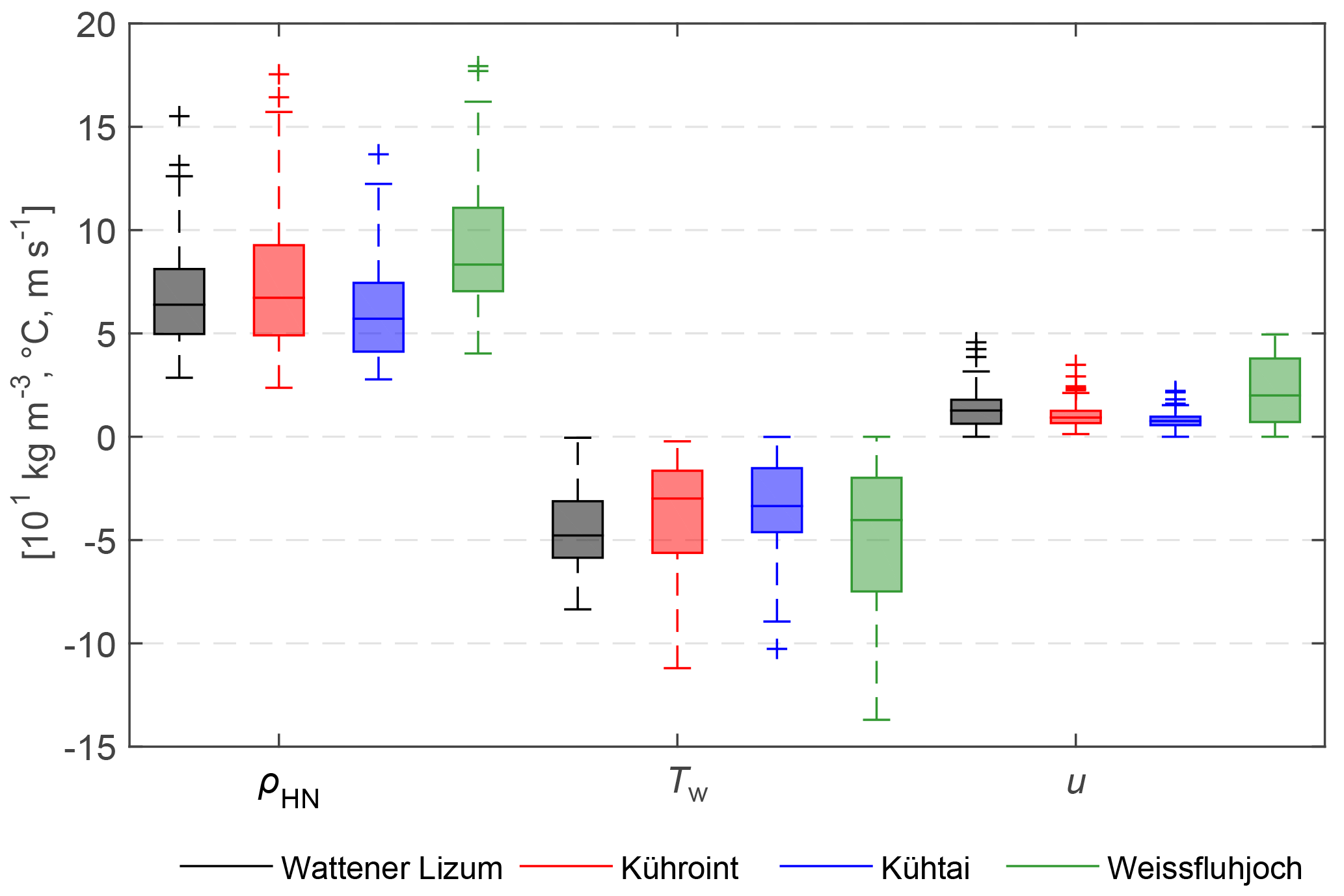
Figure 5 Box plot (median, 25 and 75 % percentiles, 1.5 × interquartile ranges, outliers) of calculated new snow densities (ρ_HN) based on observations, wet bulb temperature (T_w) and wind speed (u) for filtered snowfall events (Table 2) at all four stations within period 1 (1 October 2013–20 May 2015).

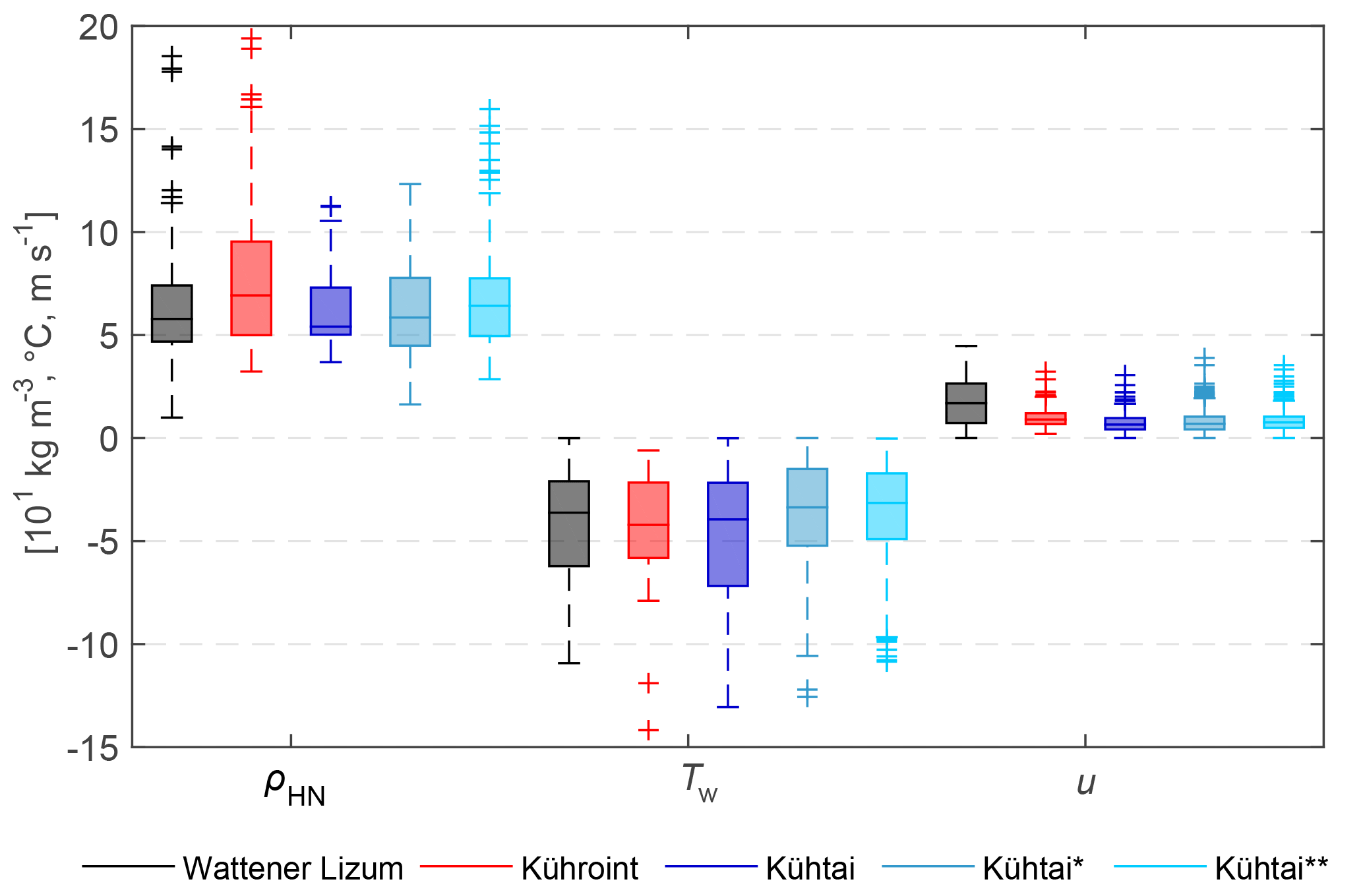
Figure 6 Box plots (median, 25 and 75 % percentiles, 1.5 × interquartile ranges, outliers) of calculated new snow densities (ρ_HN) based on observations, wet bulb temperature (T_w) and wind speed (u) for filtered snowfall events (Table 2) at three stations within period 2 (1 October 2011–1 October 2013) and at Kühtai station within period 3 (index^*, 1 October 1999–30 September 2011) and period 4 (index${}^{**}$, 27 February 1987–30 September 1999).

Wind influence may be the reason for higher ρ_HN at Weissfluhjoch station. Snow grains are fragmented by snow drift (e.g. Sato et al., 2008), and thus more packed into the layer of new snow during windy conditions even over the course of only 1 h. The Kühtai station shows the lowest ρ_HN, and the difference of the mean ρ_HN is 17 kg m⁻³ between Weissfluhjoch and Kühtai stations for period 1. Median ρ_HN and median T_w of the different periods show a relationship between the periods at Kühtai station, with a higher ρ_HN for a higher T_w (Fig. 6, Table 2).

The overall mean hourly ρ_HN of all stations and time periods is 68 kg m⁻³, with a standard deviation of 9 kg m⁻³. In general, this is considerably lower than new snow densities from daily measurements (e.g. Roebber et al., 2003; Egli et al., 2009; Teutsch, 2009). Meister (1985) measured ρ_HN lower than 100 kg m⁻³ on a daily basis, analysing data with a HN of more than 0.1 m. In contrast, the presented ρ_HN values are closer to the time of the snowfall event, and density changes over several hours due to e.g. energy exchanges and wind drift at the uppermost snow layer can be excluded. On the basis of ρ_HN in situ measurements in hourly resolution Lehning et al. (2002) emphasized that at sub-daily time intervals, lower densities in comparison to daily new snow densities have to be applied. Comparatively low ρ_HN values close to 50 kg m⁻³ were also presented by Ishizaka et al. (2016), with an average ρ_HN of 52 kg m⁻³ for aggregated snowflakes and 55 kg m⁻³ for small hydrometeors. They further found a mean ρ_HN of 72 kg m⁻³ for a second group of smaller crystals and 99.4 kg m⁻³ for graupel-type hydrometeors.

The observed inter-station variability shows the importance of differing ρ_HN between more windy mountain stations and less windy stations in the valleys.

3.3 Density parameterizations

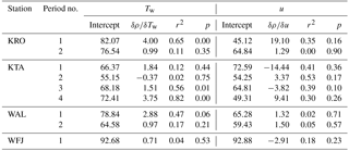
A simple linear regression analysis showed that the short-term variability of ρ_HN cannot be explained with corresponding changes in T_w or u (Table 3, Figs. 7 and S18 to S26). An increase of ρ_HN with increasing T_w can be identified in the figures, and the slopes of the least squares regressions show an increase of ρ_HN with an increase of wet bulb temperature for all stations (Table 3). However, no consistent relationship between ρ_HN and u could be found, either for single stations or for different periods at one station. The binned analysis based on T_w showed a considerable r² of more than 0.5 on a 0.01 significance level at Kühroint and Kühtai station, with intercepts of 70 to 80 kg m⁻³ and gradients of about 3 to 4 kg m⁻³ per 1 ^∘C.

Table 3 Results of a single linear regression between the corrected densities (ρ_HN) as a dependent variable and wet bulb temperature (T_w) and wind speed (u) as explanatory variables for the class median values based on all filtered data points binned into 0.5^∘ K classes and classes of 0.5 ms⁻¹, respectively. The corresponding coefficient of determination (r²) and the p value are presented.

Although the regressions generally show the expected trends, it must be noted that the variability of ρ_HN remains unexplained. This could partly be attributed to the measurement uncertainties. However, the variability caused by measurement uncertainties is assumed to be equalized, only considering the mean and median of ρ_HN values for total time periods. Relationships between ρ_HN and T_w were recognized for distinct periods and stations only, but with similar coefficients of determination in comparison to the results of e.g. Judson and Doesken (2000), Wetzel et al. (2004) or Wright et al. (2016).

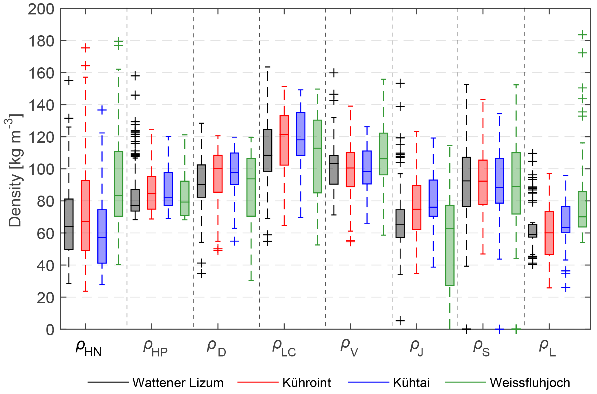
Figure 7 Box plots (median, 25 and 75 % percentiles, 1.5 × interquartile ranges, outliers) of calculated new snow densities (ρ_HN) based on observations and densities calculated using parameterizations developed in previous studies (Eqs. 3–9) at all four stations within period 1 (1 October 2013–20 May 2015).

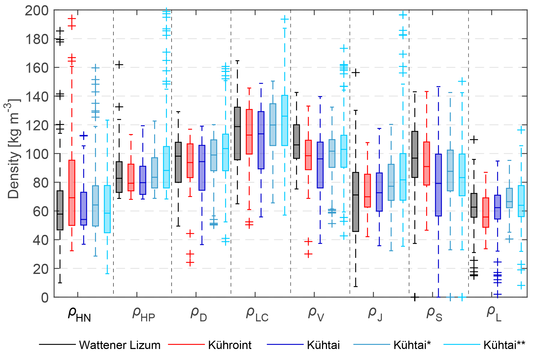
Figure 8 Box plots (median, 25 and 75 % percentiles, 1.5 × interquartile ranges, outliers) of calculated new snow densities (ρ_HN) based on observations and densities calculated using parameterizations developed in previous studies (Eqs. 3–9) at three stations within period 2 (1 October 2011–1 October 2013) and at Kühtai station within period 3 (index^*, 1 October 1999–30 September 2011) and period 4 (index${}^{**}$, 27 February 1987–30 September 1999).

Testing multiple regressions using additional meteorological parameters did not increase the statistical significance. Instead, a comparison to existing parameterizations of ρ_HN was performed for all stations and periods.

Considering the various parameterizations, which use meteorological parameters to approximate new snow density (Eqs. 3 to 9), it is evident that the observed variability of ρ_HN is not correlated to the variability of parameterized new snow densities (Table 4). Most of the seven parameterizations overestimate the median of the observed ρ_HN values (Figs. 3, 7 and 8 and Table 4). However, some parameterizations produce considerably better results than others for median ρ_HN values. The parameterizations of LaChapelle (1962), Diamond and Lowry (1954) and Vionnet et al. (2012) consistently overestimate ρ_HN. The parameterization of Hedstrom and Pomeroy (1998) overestimates ρ_HN at Kühroint, Kühtai and Wattener Lizum stations (Figs. 7 and 8), but converges with the median ρ_HN at Weissfluhjoch station for period 1 (Fig. 7, Table 4). In general, the ρ_HN values simulated using the parameterization of Jordan et al. (1999) are closer to calculated ρ_HN, but median ρ_HN values are underestimated for Weissfluhjoch station. Median ρ_HN values and the range of ρ_HN at Weissfluhjoch are well simulated using the parameterization of Schmucki et al. (2014), but it overestimates median ρ_HN of Kühroint, Kühtai and Wattener Lizum stations (Figs. 3 and 7 and Table 4). However, this parameterization was fitted to original density data from Weissfluhjoch.

Table 4 Comparison of corrected density values (ρ_HN, (kg m⁻³)) and parameterizations, applying Eqs. (3) to (9) presented in Sect. 2. Median values (m, (kg m⁻³)) are shown together with the Pearson correlation coefficient (r) and the root mean squared error (RMSE, (kg m⁻³)) between the respective calculations and ρ_HN. Best values of the performance measures are highlighted for each station and time period using bold and italic numbers.

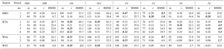
The lowest root mean squared error (RMSE) was achieved for Weissfluhjoch station with the parameterization of Diamond and Lowry (1954). The parameterizations of Lehning et al. (2002) and Jordan et al. (1999) result in the lowest RMSE (Table 4) compared to ρ_HN at Kühroint, Kühtai and Wattener Lizum stations, with slightly lower density values using the parameterization of Lehning et al. (2002) fitting best to the low median ρ_HN values of the Kühtai station.

Thus, the parameterization of Lehning et al. (2002) appears to be the first choice regarding the calculation of hourly new snow densities for high elevations and inner-alpine regions. This parameterization requires multiple input parameters. Where such data are not available, the parameterization of Jordan et al. (1999), requiring temperature and wind data only, might be a good alternative. Even though correlations are low in general, some of the highest Pearson correlation values (r, Table 4) were achieved by applying the simpler, linear equations by Diamond and Lowry (1954), LaChapelle (1962) and Vionnet et al. (2012). In addition to the regressions presented in Table 3, this shows again the identifiable relation between snow density and temperature.

Mair et al. (2016) evaluated some of the parameterizations also considered in this study. Using a distinctly larger time window for smoothing their HS data (5 h average), they calculated median ρ_HN between 75 and 100 kg m⁻³ using the parameterizations of Jordan et al. (1999) and Hedstrom and Pomeroy (1998), which is close to the results presented in this study. They also found that using the parameterization of LaChapelle (1962) results in a mean ρ_HN higher than 100 kg m⁻³. In general they concluded that using a constant ρ_HN of 100 kg m⁻³ caused an overestimation of seasonal precipitation by up to 30 %. Conversely, a mean ρ_HN of 70 kg m⁻³ will result in better SWE estimations. This is in accordance with the resulting average ρ_HN of 68 kg m⁻³ calculated from automated measurements within our study.

4 Conclusion

The aim of this study was to assess the value of automated measurements of snow depth (HS) and snow water equivalent (SWE) to compute new snow density (ρ_HN) on an hourly time interval. Complementary data sets of HS and SWE measurements using ultrasonic devices and snow pillows from four mountain stations were used to calculate the height of new snow (HN) and the water equivalent of snowfall (HNW). Subsequently, ρ_HN was calculated from HN and HNW, considering potential underestimation of HN by settling of the snowpack.

The snow measurements using ultrasonic devices and snow pillows were found to be appropriate for the calculation of station average hourly ρ_HN values. However, the observed variability in ρ_HN from the automated measurements could not be described with appropriate statistical significance by any of the investigated algorithms. An average ρ_HN of 68 kg m⁻³ with a standard deviation of 9 kg m⁻³ was calculated considering all stations and time periods. The average ρ_HN for individual stations in a common period ranged from 61 to 83 kg m⁻³, with a higher ρ_HN at more windy locations. Thus, wind speed is a crucial parameter for the inter-station variability of ρ_HN.

Seven existing parameterizations for estimating new snow densities were tested, and most calculations overestimate ρ_HN in comparison to the results from the hourly automated measurements. Two of the tested parameterizations were capable of simulating low ρ_HN at sheltered inner-alpine stations. This reveals that it has to be carefully considered which parameterization should be used for which application and environment.

Nevertheless, the natural variability of ρ_HN is masked using the combination of ultrasonic ranging and snow pillow data for ρ_HN calculation because of the limited accuracy of the sensors and snow depth changes due to settling of the snowpack and wind drift. We conclude that the value of the analysed data is given by the mean and median ρ_HN and its variation between different stations and time periods, and the considerably lower ρ_HN values in contrast to ρ_HN calculated on daily or event-based measurements.

The study shows the potential of collocated measurements of HS and SWE for determining ρ_HN automatically. However, recent developments in optical distance sensors and weighing devices increase the accuracy of such snow measurements and hence decrease the uncertainty of subsequent calculations. We therefore recommend the use of high-accuracy sensors for the determination of ρ_HN at sub-daily intervals.