the Creative Commons Attribution 4.0 License.
the Creative Commons Attribution 4.0 License.
 | 23 Apr 2018
Critical scales to explain urban hydrological response: an application in Cranbrook, London
Marie-Claire ten Veldhuis
Santiago Gaitan
Susana Ochoa Rodriguez
Nick van de Giesen
Rainfall variability in space and time, in relation to catchment characteristics and model complexity, plays an important role in explaining the sensitivity of hydrological response in urban areas. In this work we present a new approach to classify rainfall variability in space and time and we use this classification to investigate rainfall aggregation effects on urban hydrological response. Nine rainfall events, measured with a dual polarimetric X-Band radar instrument at the CAESAR site (Cabauw Experimental Site for Atmospheric Research, NL), were aggregated in time and space in order to obtain different resolution combinations. The aim of this work was to investigate the influence that rainfall and catchment scales have on hydrological response in urban areas. Three dimensionless scaling factors were introduced to investigate the interactions between rainfall and catchment scale and rainfall input resolution in relation to the performance of the model. Results showed that (1) rainfall classification based on cluster identification well represents the storm core, (2) aggregation effects are stronger for rainfall than flow, (3) model complexity does not have a strong influence compared to catchment and rainfall scales for this case study, and (4) scaling factors allow the adequate rainfall resolution to be selected to obtain a given level of accuracy in the calculation of hydrological response.
- Article
(5844 KB) - Full-text XML
-
Supplement
(20462 KB) - BibTeX
- EndNote


Rainfall variability in space and time influences the hydrological response, especially in urban areas, where hydrological response is fast and flow peaks are high (Fabry et al., 1994; Faures et al., 1995; Smith et al., 2002, 2012; Emmanuel et al., 2012; Gires et al., 2012; Ochoa-Rodriguez et al., 2015; Thorndahl et al., 2017). Finding a proper match between rainfall resolution and hydrological model structure and complexity is important for reliable flow prediction (Berne et al., 2004; Ochoa-Rodriguez et al., 2015; Pina et al., 2016; Rafieeinasab et al., 2015; Yang et al., 2016). High-resolution rainfall data are required to reduce errors in estimation of hydrological responses in small urban catchments (Niemczynowicz, 1988; Schilling, 1991; Berne et al., 2004; Bruni et al., 2015; Yang et al., 2016). New technologies and instruments have been developed in order to improve rainfall measurements and capture its spatial and temporal variability (Einfalt et al., 2004; Thorndahl et al., 2017). In particular, the development and use of weather radar instruments for hydrological applications has increased in recent decades (Niemczynowicz, 1999; Krajewski and Smith, 2005; Leijnse et al., 2007; van de Beek et al., 2010; Otto and Russchenberg, 2011; Berne and Krajewski, 2013), improving the spatial resolution of rainfall data (Cristiano et al., 2017).
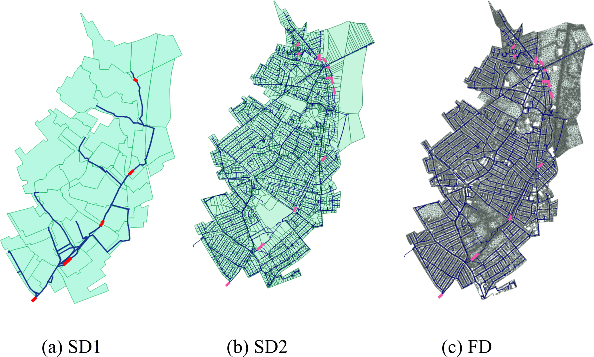
Figure 1Catchment area represented with the three different models: (a) SD1, (b) SD2 and (c) FD. The subdivision of the surface in sub-catchments or two-dimensional elements is shown for each model, as well as the sewer network. The selected 13 locations and pipes are highlighted.
The increase in high-resolution topographical data availability led to a development of different types of hydrological models (Mayer, 1999; Fonstad et al., 2013; Tokarczyk et al., 2015). These models represent spatial variability of catchments in several ways, varying from lumped systems, where spatial variability is averaged into sub-catchments, to distributed models, which evaluate the variability dividing the basin with a mesh of interconnected elements based on elevation (Zoppou, 2000; Fletcher et al., 2013; Pina et al., 2014; Salvadore et al., 2015). Salvadore et al. (2015) analysed the most used hydrological models, comparing different model complexities and approaches. An investigation of the differences between high-resolution semi-distributed and fully distributed models was proposed by Pina et al. (2016), where flow patterns generated with different model types were studied and compared to observations. This work suggested that although fully distributed models allow catchment variability in space to be represented in a more realistic way, they did not lead to the best modelling results because the operation of this type of model requires very high-quality and high-resolution data, including rainfall input.
Both rainfall and model resolution and scale are expected to have strong effects on hydrological response sensitivity. An increase in sensitivity is expected for small drainage areas and for rainfall events with high variability in space and time. Sensitivity to rainfall data resolution generally increases for smaller urban catchments. However, sensitivity of hydrological models at different rainfall and catchment scales and the interaction between rainfall and catchment variability need a deeper investigation (Ochoa-Rodriguez et al., 2015; Pina et al., 2016; Cristiano et al., 2017). This work builds upon Ochoa-Rodriguez et al. (2015), who showed that the influence of rainfall input resolution decreases with the increase in catchment area and that the interaction between spatial and temporal rainfall resolution is quite strong. We investigate the sensitivity of urban hydrological response to different rainfall and catchment scales, with the aim of answering the following research questions:
-
How should rainfall variability in space and time be classified?
-
How does small-scale rainfall variability affect hydrological response in a highly urbanized area?
-
How does model complexity affect sensitivity of model outcomes to rainfall variability?
-
How does the relationship between storm scale and basin scale affect hydrological response?
The paper is structured as follows. Section 2 presents the case study, describing the study area, models and rainfall data used in this work. Methodology applied to identify variability in space and time of model and rainfall and hydrological analysis are explained in Sect. 3. Section 4 presents the results connected to the model and rainfall variability analysis and to the hydrological analysis respectively. In Sect. 5, results are discussed, by comparing the influence of rainfall and model characteristics and identifying dimensionless parameters to describe the relation between rainfall and model scale and rainfall resolution used. Conclusions and future steps are presented in the last section.
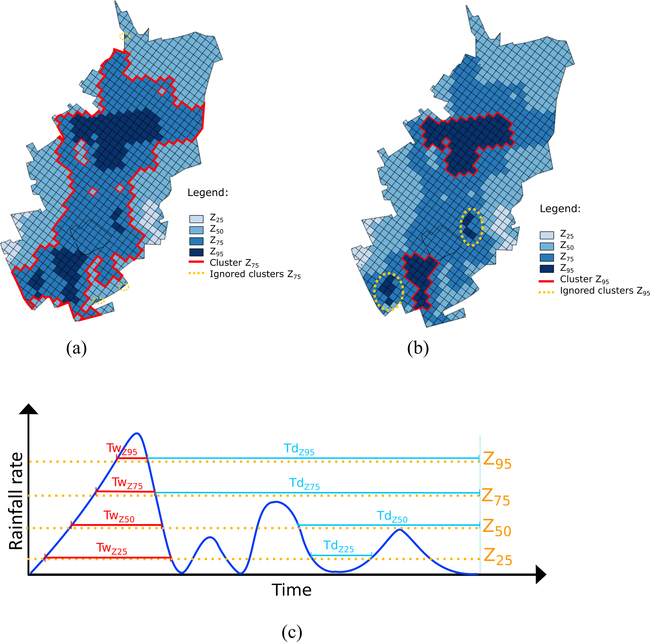
Figure 2Illustration of rainfall cluster classification. Different colours represent different rainfall thresholds. The pixels above the same threshold are used to estimate the percentage of coverage above a certain threshold. The red line encloses the clusters above threshold Z25 and Z95 in (a) and (b) respectively. Single isolated pixels and small clusters (yellow dotted circles) are ignored. (c) Schematic representation of maximum wet period (red) and maximum dry period (light blue) for a pixel, for each threshold.
2.1 Study area and available models
The city of London (UK) is exposed to high pluvial flood risk in the last years. The Cranbrook catchment, in the London borough of Redbridge, is a densely urbanized residential area. For this reason, it has been chosen as study area. A total area of approximately 860 ha is connected to the drainage network, and rainfall is drained with a separate sewer system.
For this small catchment, several urban hydrodynamical models have been set up in InfoWorks ICM (Innovyze, 2014). Three models with different representations of surface spatial variability, are used in this study: simplified semi-distributed low resolution (SD1), semi-distributed high resolution (SD2) and fully distributed two-dimensional high resolution (FD).
Table 2 summarizes the main characteristics of the three models: number of nodes, pipes and sub-catchments, dimensions of sub-catchments, two-dimensional surface elements, and degree of imperviousness. The first model, SD1, is a low-resolution semi-distributed model, initially setup by the water utility (Thames Water) back in 2010 to gain a strategic understanding of the catchment. This model divides the area into 51 sub-catchments, connected with 242 nodes and 270 pipes, for a total drainage network length of just over 15 km. The other two models, SD2 and FD, have been developed at Imperial College London (Simões et al., 2015; Wang et al., 2015; Ochoa-Rodriguez et al., 2015; Pina et al., 2016). SD2 and FD share the same sewer network design (6963 nodes and 6993 pipes), but use different surface representations. In SD2 the drainage area is divided into 4409 sub-catchments, where rainfall runoff processes are modelled in a lumped way and wherein rainfall is assumed to be uniform. In FD, instead, the surface is modelled with a dense triangular mesh (over 100 000 elements), based on a high-resolution (1 m × 1 m) digital terrain model (DTM). The rainfall–runoff transformation is different for the two types of models. For SD2, runoff volumes are estimated from rainfall depending on the land use type and routed, while for FD, runoff volumes are estimated and applied directly on the two-dimensional elements of the overland surface. Figure 1 illustrates how the surface area is modelled for each of the three models and sewer networks.
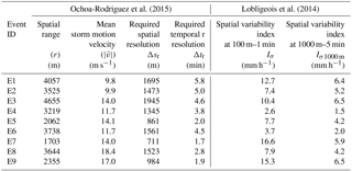
Ochoa-Rodriguez et al. (2015)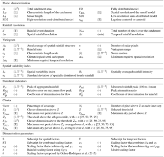
2.2 Rainfall data
Cranbrook was chosen for this study because of the availability of high-quality models at different spatial resolutions. However, for this study area, only low-resolution rainfall data were available. For this reason, rainfall events measured at a different location, with similar climatological characteristics, were synthetically applied over the Cranbrook catchment. Rainfall events were selected from a dataset collected by a dual polarimetric X-Band weather radar instrument located in Cabauw (CAESAR weather station, NL), considering that the Netherlands and United Kingdom are both in the European temperate oceanic climate (Cfb, following the Köppen classification Kottek et al., 2006). For technical specifications of the X-band radar device see Ochoa-Rodriguez et al. (2015). The selected events were measured with a resolution of 100 m × 100 m in space and 1 min in time, much higher than what is obtained with conventional radar networks (1000 m × 1000 m and 5 min). Rainfall data were applied to the Cranbrook catchment, using 16 combinations of space and time resolution aggregated from the 100 m–1 min resolution: four spatial resolutions, Δs, (100, 500, 1000 and 3000 m) with four temporal resolutions, Δt, (1, 3, 5 and 10 min) (see Ochoa-Rodriguez et al., 2015 for a motivation of the different resolution combinations). Nine rainfall events, measured between January 2011 and May 2014, were used as model input in this study. Storm characteristics are presented in Table 3.
Table 2(a) Summary of the hydrological model characteristics of the three models. (b) Drainage area connected to the investigated locations for each model.
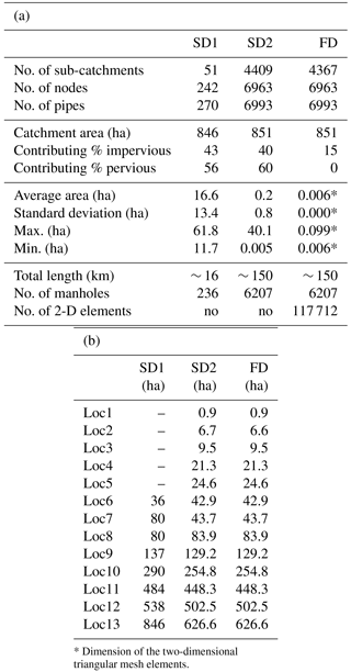
* Dimension of the two-dimensional triangular mesh elements.
In this section, different ways of classifying spatial and temporal rainfall scale are described, as well as some possible classification of catchment characteristics. We propose a new characterization of spatial and temporal rainfall variability, based on the percentage of coverage above selected thresholds. Table 1 presents the list of symbols and abbreviations used in this work.
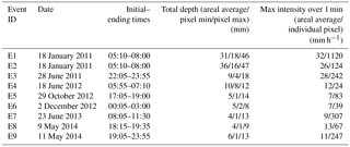
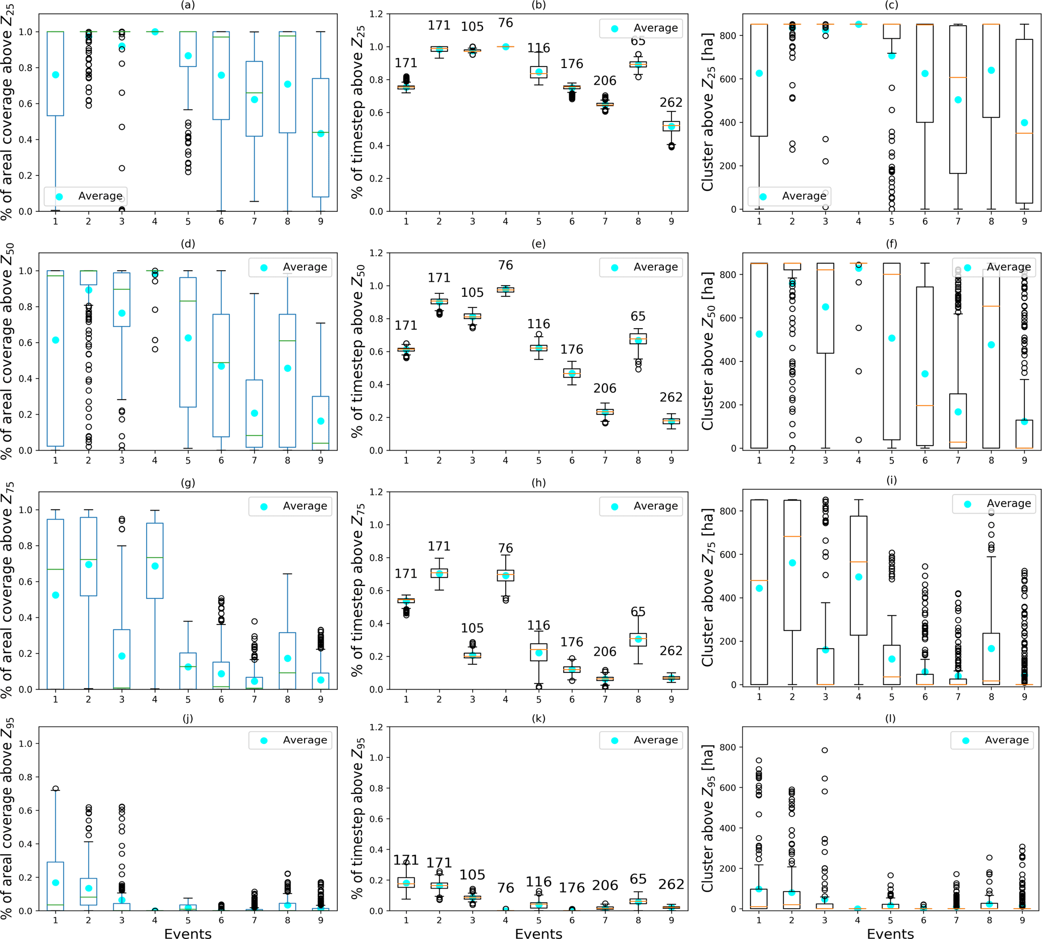
Figure 3Percentage of areal coverage above selected threshold, calculated over all time steps and per rainfall event (a, d, g, j). Temporal percentage of coverage above the selected threshold, defined as number of time steps above the threshold at each pixel, divided by the total duration of the event (b, e, h, k). Temporal percentage is presented for each rainfall event and the number above each box plot indicates the total duration of the rainfall event. Cluster dimensions across all time steps per event for the four selected thresholds (c, f, i, l). Blue dots represent the average, green or red lines the median, boxes indicate the first to third quartile, and whiskers extend 1.5 times the interquartile range below the first and above the third quartile.
3.1 Characterizing storms' spatial and temporal rainfall scale
3.1.1 Spatial rainfall scale based on climatological variogram
We computed spatial-scale characteristics based on a climatological variogram, following the approach outlined by Ochoa-Rodriguez et al. (2015). Ochoa-Rodriguez et al. (2015) presented the theoretical spatial rainfall resolution required for an hydrological model in urban area, deriving it starting from a climatological (semi-) variogram. The (semi-) variogram γ was calculated at each time step as follows:
where n is the number of radar pixel pairs located at a distance h, R is the rainfall rate and x is the centre of the given pixel, normalized by the sample variance and averaged over the time period. The obtained variogram, characteristic of the averaged rainfall spatial structure during the peak period, was then fitted with an exponential variogram and the area A under the correlogram was calculated for the exponential variogram as . Ar can be considered as the average area of spatial rainfall structure estimated with radar measurements over the study area (Ochoa-Rodriguez et al., 2015). Characteristic length scale rc [L] of a rainfall event was defined as , where r [L] is the variogram range. Minimum required spatial resolution Δsr was defined in this work as half of the storm characteristic length scale:
This parameter describes the spatial variability of the rainfall event core.
3.1.2 Rainfall spatial variability index
Another parameter to quantify and compare the spatial variability of rainfall is the spatial rainfall variability index Iσ. This parameter was at first proposed by Smith et al. (2004), called index of rainfall variability, and then recently redefined by Lobligeois et al. (2014). This index was estimated as follows:
where σt is the standard deviation of spatially distributed hourly rainfall across all pixels in the basin, per time step t, and Rt represents the spatially averaged rainfall intensity per time step. As can be seen, Iσ corresponds to a weighted average, based on instantaneous intensity, of the standard deviation of the rainfall field during a given storm event. Small values of Iσ indicate a low rainfall variability, typical of stratiform rainfall events. Large values of Iσ generally represent convective storms, characterized by high spatial variability. In the study presented by Lobligeois et al. (2014), Iσ was applied to rainfall data measured in a French region with a resolution of 1000 m–5 min and it varied between 0 and 5.
3.1.3 Storm motion velocity and temporal rainfall variability based on storm cell tracking
Ochoa-Rodriguez et al. (2015) presented a characterization of storm motion and a definition of the minimum required temporal resolution. Storm motion was defined applying the TREC method (TRacking Radar Echoes by Correlation) proposed by Rinehart and Garvey (1978) This method allows a vector representing storm motion velocity magnitude and direction of the rainfall event to be obtained at each time step. The minimum required temporal resolution, Δtr, was obtained considering time that a storm needs to pass over the storm event characteristic length scale rc. The term Δtr can be written as follows:
where [L T−1] corresponds to the mean storm motion velocity magnitude, and is obtained from the average of the storm motion velocity vectors, estimated at each time step during the peak period.
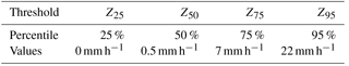
3.1.4 Rainfall spatial scale based on fractional coverage of basin by storm core
In this work, a different approach to classify rainfall events is presented, considering storm spatial and temporal variability in combination with rainfall intensity thresholds. To select the thresholds Z for the nine rainfall events over the radar grid (6 km × 6 km), percentiles at 25, 50, 75 and 95 % of the entire 100 m–1 min resolution rainfall dataset were calculated. In this way it was possible to calculate the different thresholds and Z95, corresponding to the 25th, 50th, 75th and 95th percentiles.
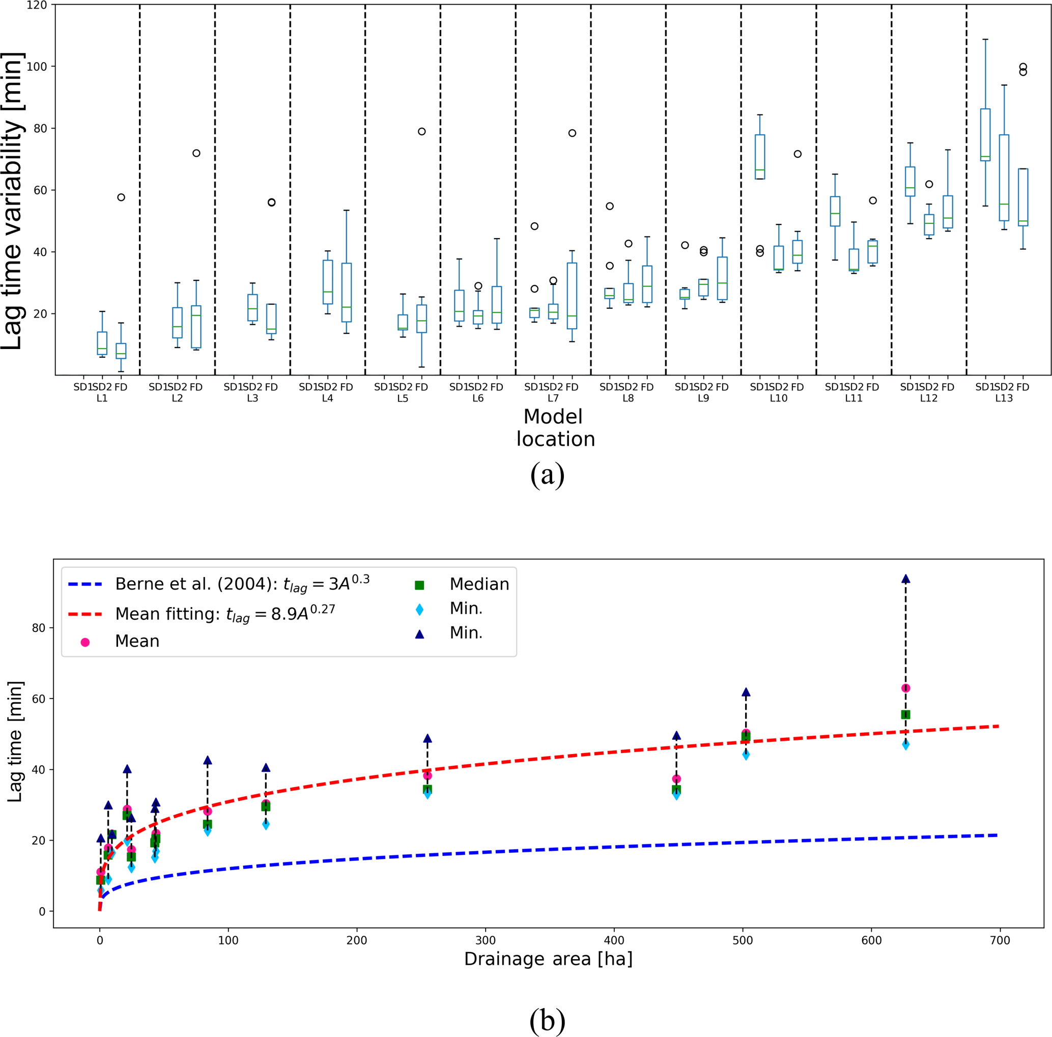
Figure 4Variability of the lag time, depending on the location, for each model (a). The box plots represent the median (red line), the upper (third quartile) and lower (first quartile) quartile (boxes boundaries), and 1.5 times the interquartile range below the first and above the third quartile (whiskers). Drainage areas corresponding to each location are presented in Table 2b. Average, median, minimum and maximum value of the lag time as a function of Ad for SD2. (b) Fitting power law curves and the power law relation proposed by Berne et al. (2004) are plotted.
Fractional coverage was largely studied in the literature and it was shown that it has a strong influence on flood response (Syed et al., 2003; ten Veldhuis and Schleiss, 2017). The percentage of coverage %cov used in this study, was defined as the sum of the number of pixels Nt above a threshold at each time step t divided over the total number of pixels of the catchment Ntot and over the total number of time steps d of the event:
The percentage of coverage was calculated for each event, in order to give a first classification of the spatial rainfall variability.
3.1.5 Rainfall cluster classification
Since variograms provide a strongly smoothed measure of rainfall field, we used alternative metrics to characterize the space scale and timescale of storm events based on cluster identification. To analyse the spatial variability of the storm core, we identified, for each rainfall event, the main rainfall cluster dimension SZ above the selected thresholds Z, as defined in Sect. 3.1.4.
For each time step, the area covered by rainfall above a certain threshold was considered. Main clusters were defined as the union of rainfall pixels above a given threshold. To identify the clusters, an algorithm based on Cristiano and Gaitan (2017) has been used. The algorithm executes the following rules:
-
All pixels above a certain threshold are considered.
-
A pixel is included in the cluster if at least one of its boundaries borders the cluster.
-
Small clusters, with an area smaller than 9 ha (about 1 % of catchment area) are ignored.
-
In the case of more than one cluster, the average of cluster areas is considered, in order to compare the cluster size at different time steps. This happens in only a few cases.
To obtain a characteristic number for each storm, cluster sizes per time step were averaged over the entire duration of rainfall event. Figure 2 presents an example of rainfall coverage at a time step t. Rainfall was divided considering different thresholds and the red line highlights the cluster for Z75 in Fig. 2a and for Z95 in Fig. 2b. The clusters identified with yellow circles are ignored because they are too small to give a considerable contribution. In a case in which there is more than one cluster, as for Fig. 2b, the average of the main clusters is considered.
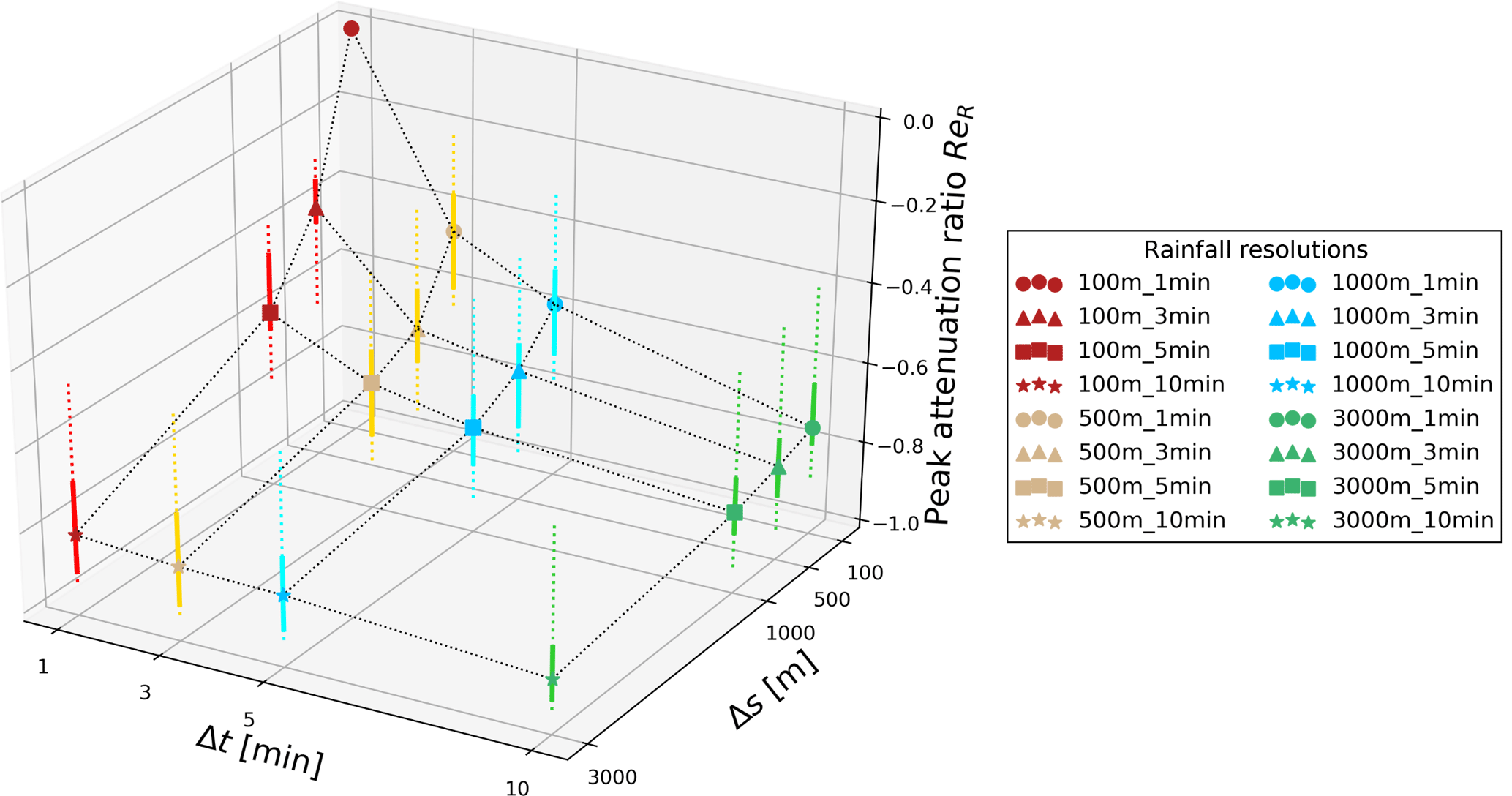
Figure 5Peak attenuation ratio ReR for the nine rainfall events, as a function of temporal and spatial rainfall resolution. Symbols indicate the median over the nine events, solid lines represent the first to the third quartile, dotted lines vary from minimum to maximum. Colours represent different temporal resolutions and markers used for the median indicate different spatial resolutions.
3.1.6 Maximum wetness period above rainfall threshold
To identify the characteristic timescale of rainfall events, maximum wetness periods were defined as the number of time steps estimated for which rainfall at a pixel is constantly above a given threshold. With this aim, every pixel in the catchment was analysed and maximum number of consecutive time steps above the chosen threshold was retrieved. Figure 2c illustrates the process followed to select the maximum duration above the threshold Z. For each pixel, the value of the maximum duration above the threshold is identified. These values are averaged over the whole catchment to obtain a temporal length scale that characterizes rainfall event .
For each pixel n, the maximum wetness period above a selected threshold Z is defined as , where Ntot is the total number of pixels.
In order to characterize the intermittency of rainfall events, the maximum dry period , defined as the maximum number of time steps during which the threshold Z was not exceeded, was also identified. Figure 2c shows how these lengths, and , were selected. The combination of these two parameters gives an indication of how constant or intermittent is the rainfall event.
3.2 Characterizing hydrological models' spatial and temporal scales
3.2.1 Models' spatial scales
Several studies have shown that drainage area is one of the dominating factors affecting the variation in urban hydrological responses resulting from using rainfall at different spatial and temporal resolutions as input (Berne et al., 2004; Ochoa-Rodriguez et al., 2015; Yang et al., 2016). Considering a larger drainage area implies aggregating and averaging rainfall and consequently smoothing rainfall peaks, with the result of having large areas that are less sensitive to high-resolution measurements.
In order to compare spatial scale of models and rainfall spatial variability, the average dimension of sub-catchments was analysed to characterize the model spatial scales. To investigate the effects of the drainage area Ad on hydrological response sensitivity, 13 locations, with connected surface that varies from less than 1 ha to more than 600 ha, were considered. Given that the coarser resolution model (SD1) does not contain small drainage areas (< 35 ha), only 8 of the 13 selected locations were available for SD1. To compare FD with SD models, we assumed that FD sub-catchments have the same dimension of SD2 sub-catchments. Table 2b presents the drainage area Ad connected to each location, while in Fig. 1 the location of the selected pipes is highlighted on the catchment with a thick red line.
Ochoa-Rodriguez et al. (2015)Lobligeois et al. (2014)Table 4Rainfall spatial and temporal characterization proposed by Ochoa-Rodriguez et al. (2015) and rainfall spatial variability index proposed by Lobligeois et al. (2014).
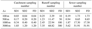
Dimensionless parameters as proposed by Bruni et al. (2015) and Ogden and Julien (1994) were determined to investigate the interaction and relation between rainfall resolution and different model properties and characteristics. The catchment sampling number was introduced as the ratio of the rainfall spatial resolution Δs to the characteristic length of the catchment LC (square root of the total area). This parameter describes the interaction between rainfall resolution and study area. If the catchment sampling number is higher than 1, rainfall variability is insufficiently captured and for small rainfall events the position might not be properly represented. The runoff sampling number was defined as , where LRA indicates the spatial resolution of the runoff model, defined as the square root of the averaged sub-catchment size (Bruni et al., 2015). Lower values of this ratio indicate that the model is unable to capture rainfall variability, while higher values indicate possible incorrect transformation of rainfall into runoff. The sewer sampling number describes the interaction between rainfall resolution and sewer length LS, indicating higher sensitivity to rainfall variability with increasing values of this ratio.
3.2.2 Models' temporal scales
In the literature, there is no unique parameter to characterize the temporal variability of the model. Several authors have proposed different timescale characteristics (see Cristiano et al., 2017 for a review), but no unique formulation has been chosen yet, especially for urban areas. Time of concentration (McCuen et al., 1984; Singh, 1997; Musy and Higy, 2010) and lag time (Berne et al., 2004; Marchi et al., 2010) are the most commonly used temporal model scales, but other time lengths have been proposed in the literature (Ogden et al., 1995; Morin et al., 2001). In this study, temporal variability of the three models was classified using lag time tlag, which describes the runoff delay compared to rainfall input. The variable tlag can be defined in different ways: as the difference between the centroid of the hyetograph and the centroid of the hydrograph (Berne et al., 2004), or as the distance between rainfall and flow peaks (Marchi et al., 2010; Yao et al., 2016). The hyetograph in a specific location was estimated as the average of rainfall intensity in the considered sub-catchment, while the hydrograph was represented using the flow in selected pipes. The lag time can be considered as a characteristic basin element. It depends on drainage area size, slope and imperviousness (Gericke and Smithers, 2014; Morin et al., 2001; Berne et al., 2004; Yao et al., 2016), but it is also influenced by rainfall characteristics. For this reason, tlag was calculated for the nine rainfall events and the average of these values was taken as the representative number.
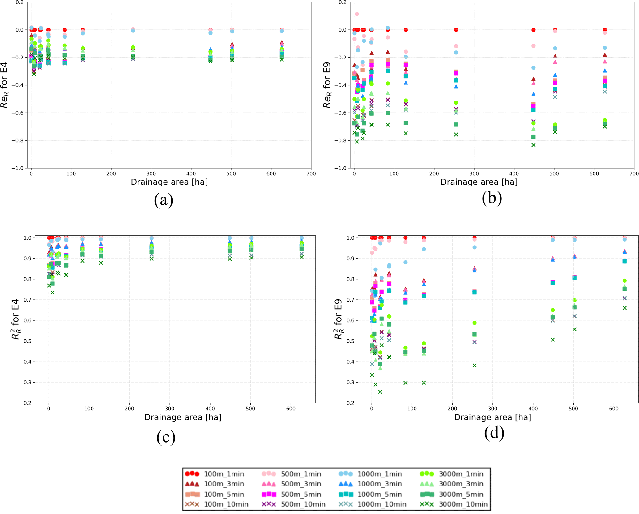
Figure 6Impact of aggregation in space and time on rainfall peak (ReR) and overall pattern () for two selected events, as a function of sub-catchment size (Ad). E4 is a constant low-intensity event with low spatial variability. E9 is an example of an intermittent event, with a high storm motion velocity. Different colours and symbols indicate different rainfall resolutions used as input. Other events are presented in the Supplement.
Lag time increases with drainage area, following a power law as proposed by Berne et al. (2004). For urban areas, an empirical relation between catchment area A (ha) and lag time tlag (min) was presented:
This relation was confirmed, incorporating results obtained by Schaake and Knapp (1967) and Morin et al. (2001). tlag was calculated for each selected sub-catchment, and then compared with the rainfall temporal scale, to investigate the interaction between model and rainfall scale. The relation between averaged lag time and connected drainage area was studied at each location.
3.3 Statistical indicator for analysing rainfall sensitivity
To investigate the effects of rainfall aggregation on peak intensity, the peak attenuation ratio ReR was calculated for rainfall. This parameter represents peak underestimation when aggregating in space and time and it was defined as follows:
where Pref is the peak of the measured rainfall at 100 m–1 min resolution and Pst is the rainfall peak at the aggregated resolution s in space and t in time. ReR values vary from 0 to 1, a condition for which there is no underestimation.
The coefficient of determination was used to describe rainfall intensity sensitivity to aggregation in space and time. represents the portion of variance of dependent variables that is predictable from the independent one. This parameter indicates how well regression approximates real data points. values can vary between 1 and 0, where 1 represents the perfect match between observed rainfall values Rref and the aggregated value Rst at spatial resolution s and temporal resolution t.
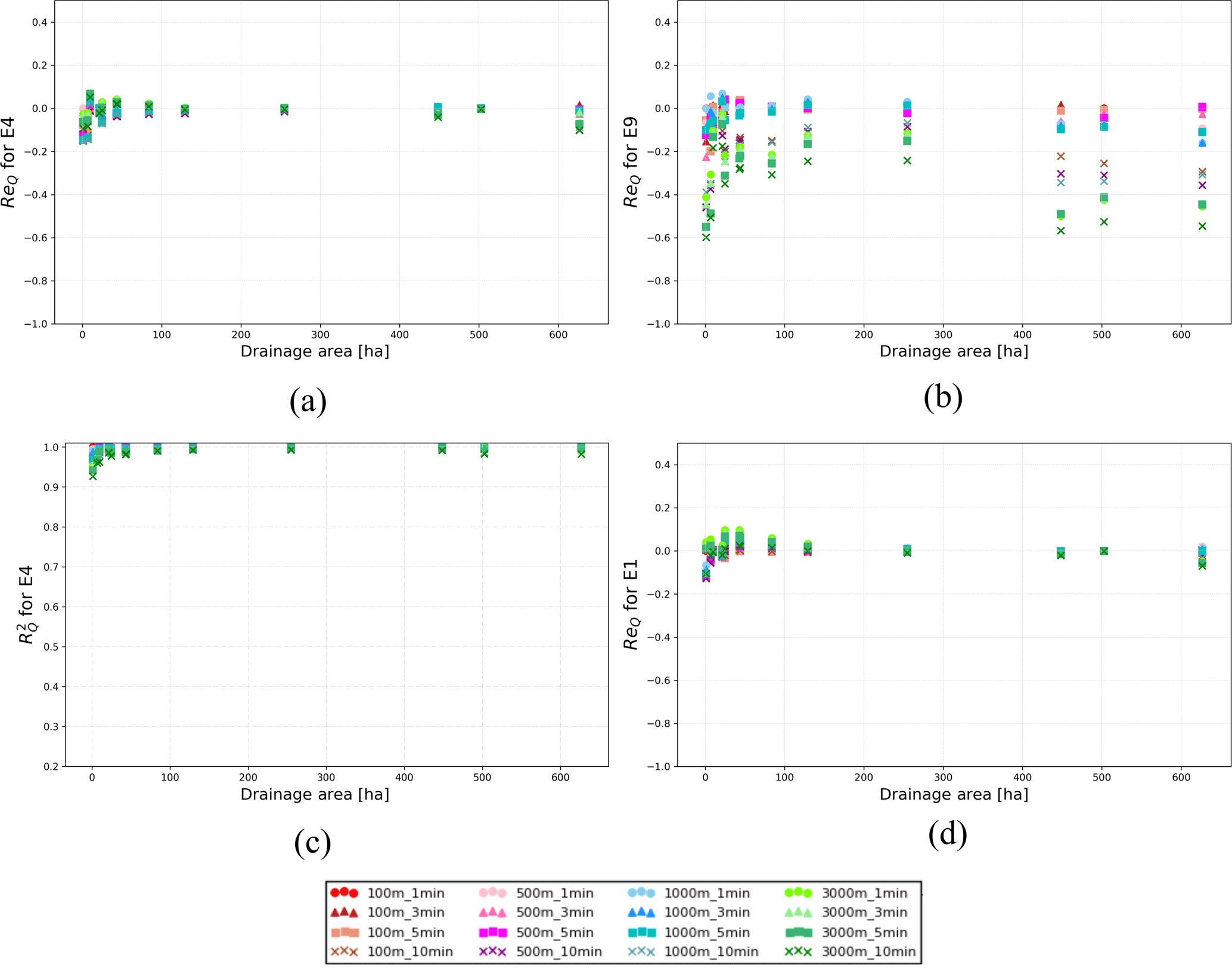
Figure 7Relative error in peak ReQ and coefficient of determination for SD2, plotted as a function of Ad, for the 16 combinations of rainfall input resolutions. Two different events are presented: E4, a low-intensity constant event, and E9, a multiple-peak event.
3.4 Statistical indicators for analysing hydrological response
Rainfall was synthetically applied over models and flow and depth were calculated in 13 selected locations, to study the hydrological response and to compare the three models. Following Ochoa-Rodriguez et al. (2015), rainfall was applied in such a way that the storm movement main direction was parallel to the main downstream direction of flow in pipes. The rainfall grid centroid coincided with the catchment centroid.
Using aggregated rainfall data as input and hydrodynamic simulation results derived from the highest-resolution rainfall (100 m and 1 min) as reference, the following two statistical indicators were calculated and analysed to quantify the influence of rainfall input resolution, at selected locations.
-
Relative error in peak flow ReQ:
where Rest is the relative error in peak () corresponding to a rainfall input of spatial resolution s and temporal resolution t, in relation to the reference (100 m–1 min) flow peak, (Ochoa-Rodriguez et al., 2015). Rest values bigger than zero indicate an overestimation of the peak associated with the rainfall input st, and, vice versa, Rest values smaller than zero indicate an underestimation. -
Coefficient of determination :
, as described in Sect. 3.3 for rainfall, was also applied to the flow, to investigate effects of rainfall aggregation on hydrological response.
3.5 Scaling factors characterizing rainfall and model scales
To investigate the impact of spatial and temporal scales of rainfall events on the sensitivity of simulated runoff to different rainfall input resolutions, Ochoa-Rodriguez et al. (2015) defined spatial and temporal scaling factors, θS and θT. These factors were defined as the ratio between required spatial and temporal minimum resolutions, Δsr and Δtr, and spatial and temporal resolutions considered as input Δs and Δt: and . The combined effects of spatial and temporal characteristics were evaluated, defining a combined spatial–temporal factor which accounts for spatial–temporal scaling anisotropy factor Ht (Ochoa-Rodriguez et al., 2015). The anisotropy factor represents the relation between spatial and temporal scales, assuming that atmospheric properties and Kolgomorov's theory (Kolgomorov, 1962) are also valid for rainfall (Marsan et al., 1996; Deidda, 2000; Gires et al., 2011). Combined spatial–temporal factor is then defined as follows: , where Ht usually assumes the value of one-third (Marsan et al., 1996; Gires et al., 2011, 2012).

Figure 8ReQ and variability, in relation to model type and rainfall characterized by cluster dimension SZ75, for all locations and all combinations of rainfall input resolution. Colours identify the three different models.
Building on the work of Ochoa-Rodriguez et al. (2015), we proposed spatial and temporal scaling rainfall factors, δS and δT. Rainfall cluster classification and maximum wetness period were used to describe the rainfall scale. The 75th percentile threshold was chosen as reference, according to the results presented in Sect. 4.4.3. The rainfall factors are defined as the ratio of cluster dimension SZ75 above Z75 to maximum wetness period above Z75 and spatial and temporal rainfall resolutions:
The characteristic spatial length of the main cluster, corresponding to the square root of the main cluster, was used to define the spatial rainfall scaling factor. Combined effects of spatial and temporal rainfall scale were investigated, defining δST as a combination of δS and δT.
The coefficient of anisotropy was not considered for the new parameters. The assumption that the anisotropy observed in the atmosphere is also present in the hydrological response is not always applicable. Results were, however, investigated with and without the anisotropy and no big differences were identified.
A similar concept was applied to model characteristics, and spatial and temporal model scaling factors were defined. These factors were obtained, comparing model characteristic length (square root of drainage area Ad) and lag time tlag with spatial and temporal resolution respectively.
The combined model scaling factor was defined as follows:
With the aim to identify a factor that represents the behaviour of hydrological response sensitivity well, three new parameters are presented. The first factor is α1, which accounts only for the spatial aspects of model and rainfall variability. The term α1 was defined as follows:
A second possible way to combine rainfall and model characteristics was α2:
In this case, both spatial and temporal aspects were considered. The catchment temporal scaling factor represents both spatial and temporal variability of the catchment, because of the strong relationship between lag time and drainage area described in Sect. 3.2.2.
The third scaling factor, α3, combines all spatial and temporal rainfall and model characteristics. The term α3 was defined as follows:
These parameters allow the best rainfall resolution or model scale to be chosen. Depending on the available data and on the level of performance that we want to achieve, it is possible to identify the required rainfall resolution.
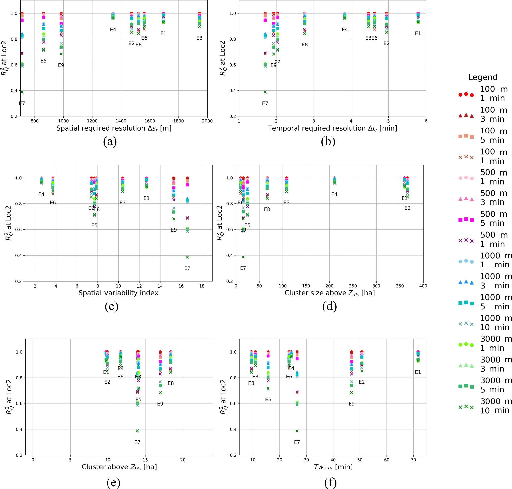
Figure 9 at Loc2 for different rainfall resolution, plotted against different rainfall characterizing scales: spatial (a) and temporal (b) required resolution, spatial variability index (c), dimension of cluster above Z75 (d) and Z95 (e), and maximum wet period above Z75 (f).
4.1 Rainfall analysis
In this section, methods for quantifying rainfall space and timescales proposed in the literature (Ochoa-Rodriguez et al., 2015; Lobligeois et al., 2014) are compared to the cluster classification we propose in this paper. Additionally, change in rainfall characteristics with spatial and temporal aggregation scale will be analysed.
4.1.1 Spatial and temporal classification results
Spatial variability index values for each of the nine rainfall events are presented in Table 4 for the observed rainfall at 100 m–1 min (Iσ) and at 1000 m–5 min (Iσ1000 m). The last two columns on the right were added to have a direct comparison with the values presented by Lobligeois et al. (2014), who used the same resolution. Iσ values are generally high when compared to values found by Lobligeois et al. (2014) for all the investigated regions. This indicates that most events are characterized by high spatial variability. Aggregation has a strong impact on this parameter, which becomes smaller with a coarser resolution, highlighting the fact that information about rainfall variability is lost during the coarsening process. Iσ1000 m values are generally higher than values presented for the northern region, where values are below 1, but are comparable to the Mediterranean area, where Iσ reaches values around 4.
Table 5Thresholds values obtained for the nine rainfall events considered.
Values obtained based on variogram analysis (spatial range) and storm tracking (temporal development) following Ochoa-Rodriguez et al. (2015) are also presented in Table 4.
Results show that the spatial variability index tends to increase as well as the required spatial resolution for storms larger than 2500 m spatial range, while events with small spatial range (E5, E7 and E9, spatial range below 2500 m) are characterized by relatively high spatial variability indexes. Required temporal resolution Δtr, obtained from the combination of storm motion velocity and required spatial resolution (see Sect. 3.1.3) varies between 1.7 and 5.9 min; the lowest values of Δtr are associated with fast storm events (e.g. E8 and E5) and small-scale events (e.g. E9 and E7).
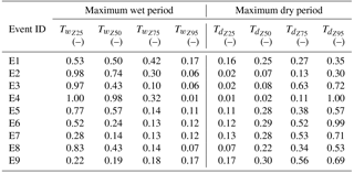
Table 6Maximum wetness periods above the threshold, calculated for each pixel, averaged over the total catchment, and then divided by the total duration.
4.1.2 Thresholds and percentage of coverage
The first step in obtaining cluster dimensions is to identify rainfall thresholds (Z) characterizing the rainfall values' distribution (see Sect. 3.1.4). Table 5 shows rainfall threshold values corresponding to the 25th, 50th, 75th and 90th percentiles for the nine rainfall events.
The 25th percentile of the rainfall values distribution is zero, indicative of strong intermittency and small areal coverage of some of the events (especially events E7 and E9). The 95th percentile is 22 mm h−1 (over a 1 min time window), corresponding to a recurrence interval of less than 6 months (KNMI, 2011), indicating that the selected events are representative of frequently occurring events. For this region, rainfall intensities above 25 mm h−1, over a 15 min time window, correspond to a return period of once per year, indicating an intense rainfall event. For only few rainfall events, E1, E2, E3 and E7, the 25 mm h−1 threshold is exceeded over a 15 min time window, for few time steps and, in particular, for E7 this happens only at the peak. This implies that rainfall events considered in this study are not classifiable as extreme.
Table 7Dimensionless parameters for the three models used in this study, based on Bruni et al. (2015), used to describe the interaction between spatial rainfall resolution and model scale.
The percentage of areal coverage, estimated for the catchment, is presented in Fig. 3a, d, g, j. Areal coverage associated with 25th percentile values provides an indication of event-scale intermittency. Events with 25th percentiles close to 1 cover the entire catchment most of the time, while smaller and more intermittent events, especially E7 and E9, are characterized by lower 25th percentile values. Areal coverage for 95th percentile thresholds indicates the size of storm cell cores: E1 and E2 have storm cores covering up to 65–70 % of the catchment; E4 and E6 have median coverage values close to zero, indicating that these are mild events without an intense storm core.
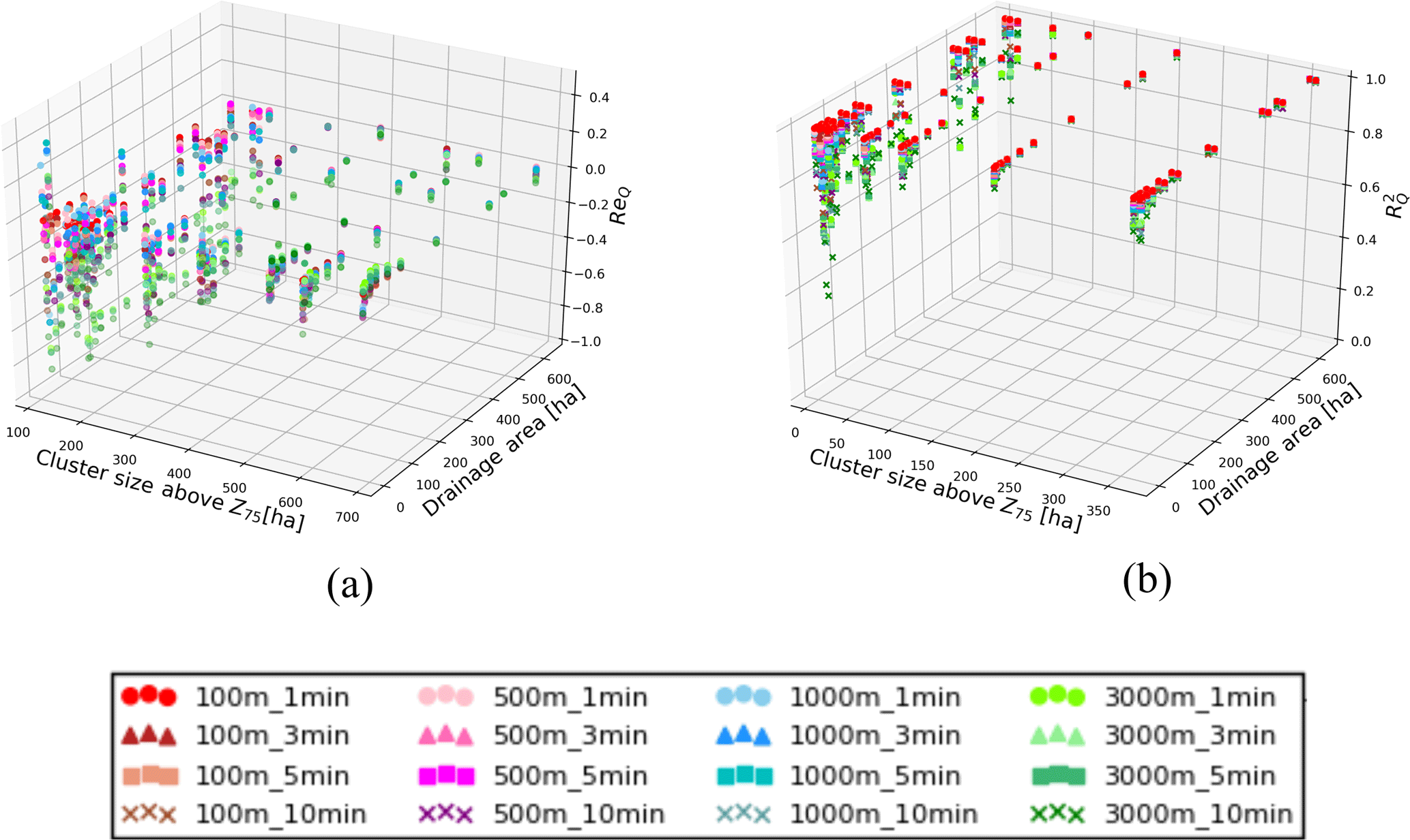
Figure 10ReQ and as a function of cluster dimension above Z75 and Ad. Different colours and symbols indicates different rainfall resolution input.
Box plots in Fig. 3b, e, h and k show the number of time steps above selected thresholds as a percentage of total event duration, to enable comparison between events. Results confirm patterns identified based on areal coverage: events E7 and E9 are identified as high-intermittency events (based on 25th percentile threshold). Maximum percentage of time steps above the highest threshold is 30 % for events E1 and E2. Each box plot represents the spatial variability of rainfall between pixels. Thresholds Z50 and Z75 present a high intra-event variability, highlighting the differences between rainfall events. For the other two thresholds, the intra-event variability is not high, suggesting that the rainfall event characteristics might not be well represented. For Z95, all events present a coverage variability lower than 30 %, and differences between events are not properly defined. Thresholds Z50 and Z75 present also a high inter-event variability, indicating that in these cases the spatial variability of the rainfall event above the catchment area is high.
4.1.3 Rainfall cluster classification
Dimensions of the main cluster were determined for each of the four thresholds and for all time steps of the nine events. Results are presented in Fig. 3c, f, i and l, where the red line indicates the median and the blue dot the average.
The plots show that for Z25 only intermittent events, like E7 and E9, present a median below 861 ha (entire catchment area). The intra-event variability is generally quite high for most of the events, especially for the 50th and 75th percentiles, indicating that clusters change their dimension and shape during the event. Only a couple of events, E4 and E2, do not show high variability above Z25 and Z50 threshold. For Z95, the cluster dimension variability is relatively small, suggesting that the average or the median can be a good approximation of the storm core dimension. Values above Z50 present high inter-event variability. There is a clear distinction between constant events, such as E2 and E4, and intermittent events, E7 and E9, which show low median and average values.
Intense and constant rainfall events are also characterized by median values being generally higher than the mean. However, intermittent events, such as E9, have an average higher than the median, especially for the 50th and 75th percentiles. These results suggest that Z50 and Z75 are able to describe rainfall spatial and temporal scale well.
4.1.4 Maximum wet and dry period
The maximum wet period and maximum dry period were calculated for four rainfall intensity thresholds in order to represent temporal variability of a rainfall event. Table 6 presents maximum wetness period and maximum dry period , normalized by total duration of the rainfall event, to enable comparison between events and to investigate how long the main core is in relation to the total duration of the event.
For some events decreases depending on the threshold, passing from values close to 1 for Z25 to values close to 0 for Z95. The change between different thresholds can be gradual, as for example for E2, E8 or E5, or sharp, as is the case of E3 or E4. For intermittent events, however, the maximum wet period does not vary too much, and it is relatively short, like E7 or E9. This implies that there are probably multiple short periods above the threshold. When comparing and , we can observe that some events show a symmetrical behaviour, when a decrease in wet period coincides with an increase in dry period, with the increase in the threshold (E4, E3). E7 and E9 present a moderate decrease in while they have a steep increase in , indicative of strong intermittency. For the other events, the behaviour is generally the opposite, indicative of a concentrated storm core.
4.2 Hydrological model, spatial and temporal scales
4.2.1 Spatial model scale
Dimensionless sampling numbers, presented at first by Ogden and Julien (1994), and then re-proposed by Bruni et al. (2015), are presented in Table 7 for the three models (for underlying equations see Sect. 3.2.1). SD2 and FD model have the same contributing area and network length, hence they show that values for the catchment sampling number and sewer sampling number are the same.
Catchment sampling numbers higher than 1 indicate that models can not properly represent rainfall variability (Bruni et al., 2015). In this study, for 3000 m spatial rainfall resolution values are bigger than 1, so poor model performance at this resolution is expected. The runoff sampling number suggests that SD1 will not be able to capture rainfall variability, because it presents low values for all spatial resolutions, while FD has high values of this parameter, which highlights some uncertainty in rainfall–runoff transformation. SD2, instead, presents runoff sampling numbers similar to the values found by Bruni et al. (2015), where this parameter varied between 2.6 for high resolution and 93 for lower resolution. The sewer sampling number applied to SD2 and FD presents similar results to Bruni et al. (2015), where the values were varying between 2 for high resolution and 77 for low resolution. However, the sewer sampling number is pretty low for SD1, which indicates a low sensitivity of this model to rainfall variability. This parameter increases with coarsening of spatial resolution, suggesting a high sensitivity to coarser rainfall resolutions.
The catchment sampling number can be applied also to the selected sub-catchments, comparing spatial resolution with the sub-catchments dimension reported in Table 2b. Also in this case, when the ratio is bigger than 1 the rainfall might not be well represented. This happens for sub-catchment L1, which is smaller than 100 m, and for all locations when they have to deal with 3000 m rainfall resolution. Locations from L2 to L5, presenting a drainage area between 100 and 500 m, should show the effects of aggregation for spatial resolution of 500 and 1000 m, when the catchment sampling coefficient is higher than 1, and the variability is not well captured. When the catchment sampling number is lower than 0.2, the catchment is too large to be compared to the rainfall input, and the effects of averaging over the area should be visible, as for example for L13 when considering a 100 m input resolution.
4.2.2 Temporal model scale
Lag time tlag was computed for 9 storms for each model at 12 sub-catchments and at the catchment outlet, as explained in Sect. 3.2.2. Results, presented in Fig. 4a, show that tlag increases with drainage area and varies from just above 1 min for FD at L1 (upstream location with the smallest Ad) to over 100 min for the coarsest model and largest catchment scale.
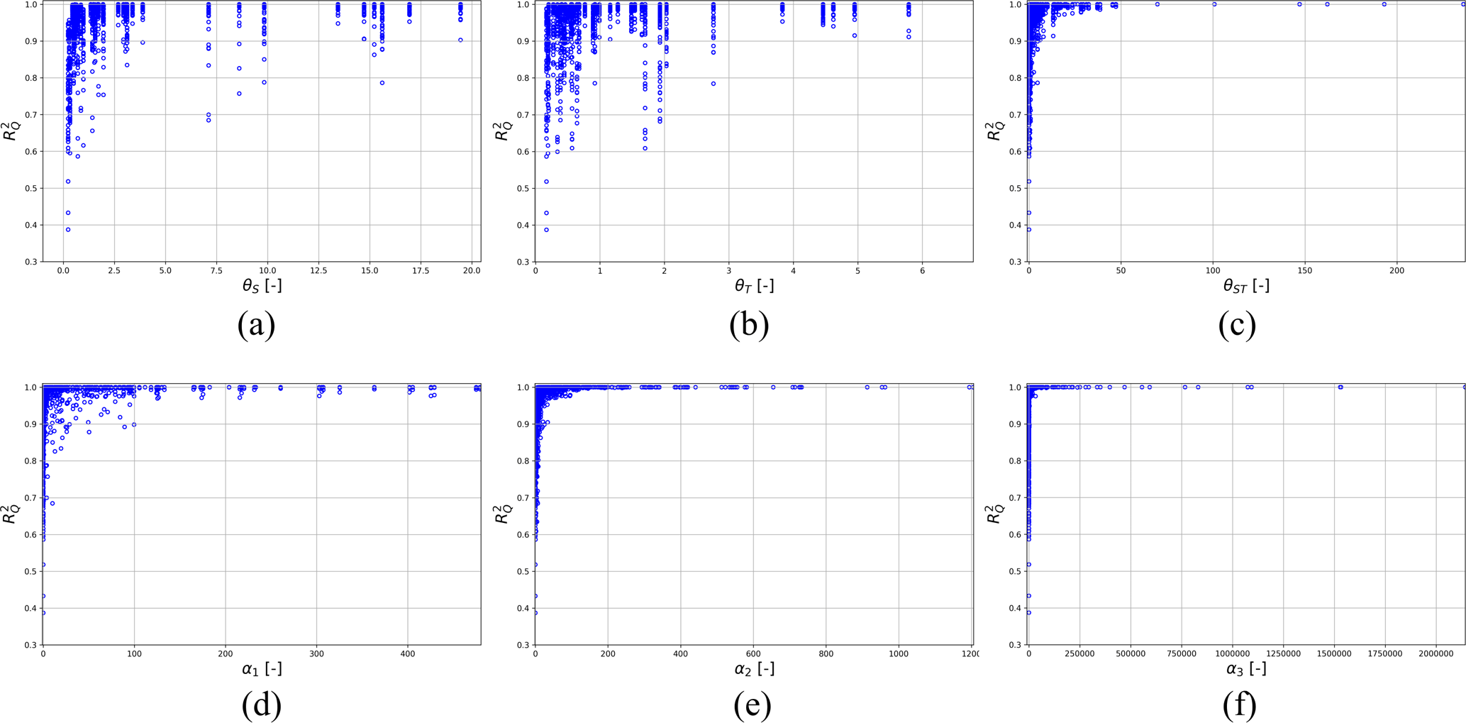
Figure 11Performance statistic as a function of dimensionless numbers θS, θT, θST, δS, δT, δST, γS, γT, γST, α1, α2 and α3. For each parameter all events, rainfall resolutions and locations are plotted.
For only a few locations, tlag is lower than 10 min and for this reason a low sensitivity to temporal variability of rainfall events is expected. However, lag times vary over a wide range between events, and this highlights a strong influence of event characteristics. Model scale clearly influences computed lag times, which are generally larger for coarser models, where sub-catchments are bigger. However, for locations with smaller drainage area (<245 ha), SD1 presents tlag values comparable with the other models, but with a much lower variability compared to the finer-scale models.
As discussed in Sect. 3.2.2, tlag strongly depends on drainage area. Figure 4b shows how lag time varies, as a function of drainage area, for SD2, based on average, median, minimum and maximum values across rainfall events. Results confirm that tlag increases with the drainage area, fitting a power law, similar to the one suggested by Berne et al. (2004) (Eq. 6). In this case the power law that fits at best the average of empirical data is (R2=0.841), an equation that presents the same exponent of the one proposed by Berne et al. (2004) and a slightly higher coefficient. The power law proposed by Berne et al. (2004) represents a wider range of surface areas wider than what is presented in this work; hence, only a small part of it is considered.
4.3 Sensitivity of rainfall: effects of spatial and temporal aggregation on rainfall peak and distribution
4.3.1 Effects of aggregating on the maximum rainfall intensity at catchment scale
Figure 5 presents rainfall peak attenuation ratios ReR for the range of spatial and temporal aggregation levels investigated. The plot shows the median over the nine events (marker) and the variability of the data (from 25 to 75 %: solid lines; total range: dotted lines).
Rainfall peaks are reduced up to 80 % when aggregating in space or time and up to 88 % when combining the spatial and temporal aggregation at the coarsest resolution. For high resolution, aggregation over time seems to play a larger role than over space. Approximately half of the rainfall peak is lost when aggregating from 1 to 3 min, while from 100 to 500 m peak attenuation is relatively smaller (40 %). For lower resolutions, spatial aggregation has a slightly stronger attenuating effect than temporal aggregation. At 3000 m spatial resolution, rainfall peaks are strongly underestimated, independent of the temporal resolution.
4.3.2 Rainfall aggregation analysis at sub-catchment scale
In this sub-section, we compare effects of spatial and temporal aggregation on rainfall variability and peak intensity across sub-catchment scales. Figure 6 shows examples of rainfall aggregation effects, as a function of the drainage area. Results for two rainfall events are shown: E4 is a constant, low-intensity event, which has a low variability in time and space, while E9 is an intermittent event, with multiple peaks. The plots clearly show that rainfall variability for the constant event is less sensitive to aggregation than that for the intermittent event. Rainfall sensitivity to aggregation decreases for larger sizes. ReR and results for all the nine studied events are available in the Supplement.
4.4 Rainfall and model influence on hydrological response
4.4.1 Sensitivity of the hydrological response to rainfall input resolution
Figure 7 shows results for statistical indicators ReQ and for 16 combinations of rainfall resolution and in relation to catchment area. Results are shown for a stratiform low-intensity rainfall event (E4) and a convective intermittent storm (E9) for increasing catchment size. For both events, the sensitivity to rainfall input resolution generally decreases with increasing catchment size. The variability of ReQ and is much stronger for E9 than E4, pointing out the important role of rain event characteristics.
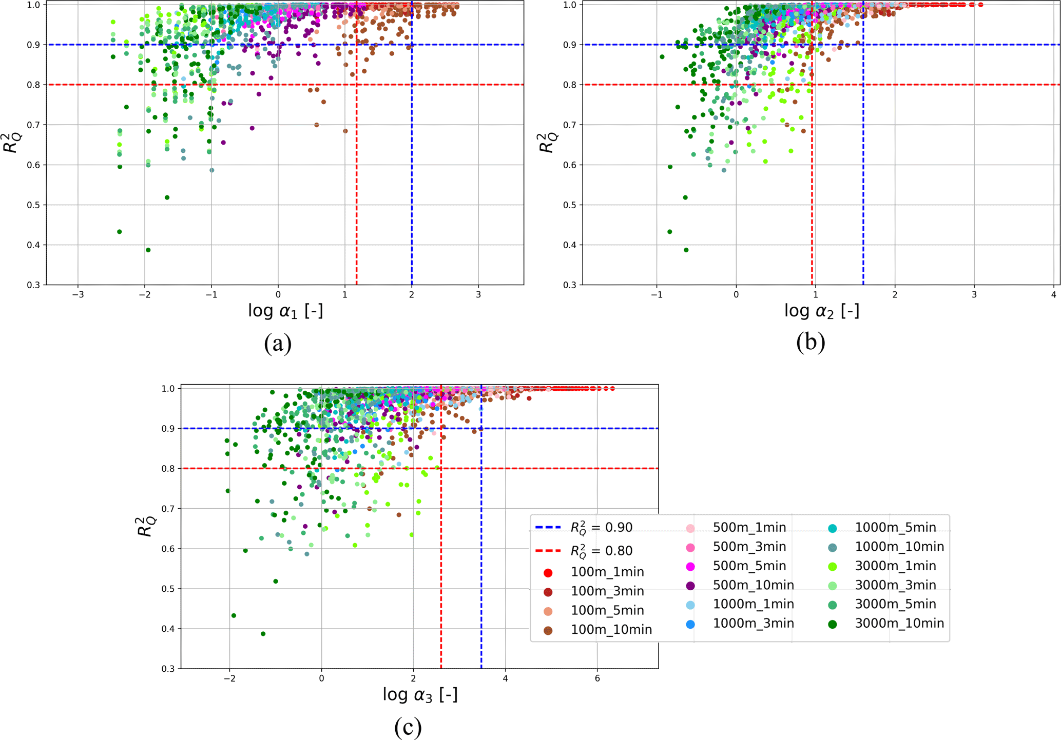
Figure 12Logarithmic plots of as a function of (a) α1, (b) α2 and (c) α3. Different colours indicate different resolutions.
Comparing Fig. 6 with Fig. 7, similar patterns are observed for rainfall and flow. In both cases, sensitivity to rainfall aggregation in space and time decreases with increases in the drainage area. Moreover, in both cases, the small and constant event (E4) is less sensitive to aggregation than the intermittent one (E9). Rainfall patterns are more sensitive to aggregation than flow, due to smoothing induced by rainfall–runoff processes.
4.4.2 Influence of the model complexity on hydrological response sensitivity
To investigate the influence that model complexity has on hydrological response sensitivity, results obtained with the three models are analysed. Figure 8 compares the influence of model complexity to the impact of spatial rainfall variability on the sensitivity of hydrological response. For each model, outputs at all locations are plotted for the 16 different rainfall input resolutions. There is not a clear behaviour that characterizes differences between sensitivity of the three models. All models appear sensitive to 3000 m spatial resolution and 10 min temporal resolution: in these cases the performance is lower. For upstream locations, SD1 seems to be slightly more sensitive than the other models to spatial coarsening for the upstream location, while FD performs worse for L13. The plot shows that there are some minor differences between the outputs of the three models, but the strongest sensitivity is connected to the rainfall scale as characterized by the cluster dimension. All models show higher sensitivity to small clusters, especially for cluster sizes below 100 ha. For small clusters, SD1 presents a higher sensitivity for both statistical indicators, while it is less sensitive than SD2 and FD for large clusters.
Model complexity does not have a large influence on sensitivity to rainfall resolution coarsening, while other characteristics, such as rainfall parameters or catchment details, seem to have a higher impact.
4.4.3 Influence of rainfall-scale classification on hydrological response
Several approaches to classifying rainfall variability have been presented and discussed in Sects. 3.1 and 4.1. In these sections, their influence on the hydrological response will be analysed.
Figure 9 compares the influence of spatial and temporal required resolutions (Δsr and Δtr), spatial variability index Iσ, cluster above Z75 and Z95, and the maximum wet period to model performance at different resolutions. Sensitivity to rainfall input resolution generally increases for smaller required spatial and temporal resolution, for higher spatial variability index, and for smaller cluster size. The clearest relationships are observed for required temporal resolution and cluster size above Z75. This parameter seems to represent spatial scale of the rainfall events quite well, and therefore it is chosen in this work to characterize the spatial scale of rainfall events.
Figure 10 compares the influence of rainfall spatial scale, based on cluster size above Z75, with drainage area size. The variability of is higher for lower values of both rainfall scale and drainage area and decreases in a similar way with increases in both rainfall and catchment dimensions.
For this case study, we can conclude that sensitivity to rainfall resolution depends mainly on the scale of rainfall events and study catchment, and much less on the complexity of the models used. Choosing a complex model is useful only when studying small-scale events and catchments and only if high-resolution rainfall data are available.
4.5 Rainfall and model scaling factors
Spatial, temporal and combined scaling factors proposed by Ochoa-Rodriguez et al. (2015) and described in Sect. 3.5, were calculated for this study and are presented in Fig. 11a–c. Higher values of the scaling factors θS (ratio of minimum required spatial resolution to rainfall spatial resolution), θT (ratio of minimum required temporal resolution to rainfall temporal resolution) and θST (combination of spatial and temporal scaling factors) are generally associated with higher modelling performance, expressed in terms of R2. The combined spatial–temporal scaling factor, θST, in particular indicates how high values are obtained for θST>15 (R2>0.9).
As discussed in Sect. 4.4.3, both rainfall scale and catchment characteristics strongly affect sensitivity of hydrological response to rainfall resolution. For this reason, the new dimensionless factors proposed combine rainfall and catchment properties. From results shown in Fig. 11a–c, spatial variability seems to have a better relation with the sensitivity variability than the temporal scale and, for this reason, the factor α1 especially focuses on the spatial scale of model and rainfall variability. Figures 11d and 12a show as a function of α1. The plot presents a clear trend, indicating low model performance for low values of α1 and high performance for values of α1 larger than 100.
Figure 11e shows α2 and response sensitivity. For values of α2>40, is higher than 0.95, indicating a very good performance. For values of α2<10, is lower than 0.8. Figure 12b shows the same plot on a logarithmic scale, which better visualizes thresholds of performance. Different resolutions are highlighted in the plot. Low resolution in space generally lead to a lower α values than low temporal resolution, and consequently to a lower performance of the model.
Figures 11f and 12c plot against α3. Figure 12c indicates that for values of α3 higher than 3000, a high performance of is guaranteed (R2>0.90). For the performance of drops to 0.8.
Comparing the scaling factors, we observe that α2 works better in distinguishing critical resolutions for a given model performance. There are indeed fewer points with high below the identified thresholds. Moreover, α2 should be preferred because it allows fewer parameters to be used, without losing information about temporal characteristics, as it is for α1.
In this study we investigated the effects of rainfall and catchment scales on sensitivity of urban hydrological models to different rainfall input resolutions. The aim was to identify dimensionless ratios of storm and catchment scales that support critical resolution for reproducing hydrological response. Cranbrook, a small urbanized area of 861 ha, was analysed with the help of two semi-distributed models and a fully distributed model. Rainfall data measured at 100 m and 1 min resolution by a dual polarimetric X-band radar instrument located in the Netherlands were aggregated to obtain different rainfall resolutions and then used as input for the hydrological models. Storm events were assumed to be representative of the rainfall regime in the London area, as London and Cabauw are situated in the same temperate oceanic climatological region. A new rainfall classification method, based on cluster identification, was presented in this work. Different rainfall classification methods were used to characterize storm event scales.
From this work we draw the following conclusions.
-
Rainfall classification based on clustering is an easy and fast method to quantify the spatial scale of rainfall events. In particular, rainfall clusters associated with the 75th percentile threshold gave a realistic approximation of the spatial dimension of the storm core.
-
Spatial and temporal aggregation of rainfall data can have a strong effect on rainfall peak and intensity. Rainfall peaks were reduced up to 80 % when aggregating in space to 3000 m resolution or in time at 10 min resolution. Both space and time have a strong influence on peak attenuation. Temporal aggregation has a stronger influence at 1–5 min resolution, while aggregation in space has bigger impact at low (1000–3000 m) resolution.
-
Lag time estimated for the investigated sub-catchments was used to represent the temporal characteristics of models. Lag time increased with the catchment area size, yet varied strongly between events (approx. by a factor of 2; 25–75th percentile range). Mean lag time fitted an empirical power law similar to the one proposed by Berne et al. (2004), yet with a higher intercept.
-
Effects of rainfall aggregation in space and time on hydrological response depend on rainfall event characteristics. Rainfall events with constant intensity are less affected by aggregation than small-scale intermittent events. However, results showed that aggregation effects are stronger for rainfall than flow. Results showed that smoothing of rainfall peak intensities by aggregation was much stronger than for flows. Rainfall aggregation effects on hydrological response are smoothed during the rainfall runoff transformation processes.
-
For the case study under consideration, model spatial resolution does not appear to have a big impact on hydrological response sensitivity to rainfall input resolution. Three models of different complexity were all sensitive to rainfall resolution. The low-resolution model was more sensitive to rainfall resolution for small-scale storms, while the high-resolution fully distributed model showed stronger sensitivity at larger catchment scale.
-
Rainfall and catchment scales were shown to have a strong impact on hydrological response sensitivity. This indicates that the relation between rainfall and catchment scale needs to be taken into account when investigating the hydrological response of a system.
-
New spatial, temporal and combined scaling factors were introduced to analyse hydrological response sensitivity to rainfall resolution. These dimensionless scaling factors combine rainfall scale, model scale and rainfall input resolution and enable identification of critical rainfall resolution thresholds to achieve a given level of accuracy. Thus, the scaling factors support the selection of adequate rainfall resolution to obtain a certain level of accuracy in the calculation of hydrological response.
However, there are still some aspects that need further investigation. Rainfall events measured directly over the study area should be evaluated to allow a proper comparison between model results and observations. In particular, using local rainfall data as input for the model, combined with local discharge measurements, would enable direct investigation of the sensitivity of the hydrological response with respect to an observed reference. Results presented in this paper are related to one specific case study and need further investigations, based on cases in different climatological regions and with different hydrological characteristics to estimate the extent to which they can be generalized. More and different rainfall events and different catchments should be investigated in order to test the applicability of the scaling factors and thresholds identified for other geographical and climatological conditions. In further work, cluster rainfall classification and dimensionless α parameters will be investigated based on field observations in combination with modelling. Different scales will be considered to investigate the range of applicability of the scaling factors. Additionally, a better definition of temporal rainfall scale needs to be developed, with a parameter that is able to represent rainfall variability, highlighting the constant or intermittent character of rainfall events.
The code used for the rainfall cluster classification is available in Cristiano and Gaitan (2017).
The supplement related to this article is available online at: https://doi.org/10.5194/hess-22-2425-2018-supplement.
The authors declare that they have no conflict of interest.
The authors would like to thank Innovyze for providing a InfoWorks licence.
This study was funded by the EU INTERREG IVB RainGain Project.
Edited by: Markus Weiler
Reviewed by: Kristian Förster and one anonymous referee
Berne, A. and Krajewski, W.: Radar for hydrology: Unfulfilled promise or unrecognized potential?, Adv. Water. Resour., 51, 357–366, https://doi.org/10.1016/j.advwatres.2012.05.005, 2013. a
Berne, A., Delrieu, G., Creutin, G., and Obled, C.: Temporal and spatial resolution of rainfall measurements required for urban hydrology, J. Hydrol., 299, 166–179, https://doi.org/10.1016/j.jhydrol.2004.08.002, 2004. a, b, c, d, e, f, g, h, i, j, k, l
Bruni, G., Reinoso, R., van de Giesen, N. C., Clemens, F. H. L. R., and ten Veldhuis, J. A. E.: On the sensitivity of urban hydrodynamic modelling to rainfall spatial and temporal resolution, Hydrol. Earth Syst. Sci., 19, 691–709, https://doi.org/10.5194/hess-19-691-2015, 2015. a, b, c, d, e, f, g, h
Cristiano, E. and Gaitan, S.: rainfall-clustering: Initial version of protocol for intensity based rainfall radar imagery clustering, Zenodo, https://doi.org/10.5281/zenodo.1069327 (last access: 28 December 2017), 2017. a, b
Cristiano, E., ten Veldhuis, M.-C., and van de Giesen, N.: Spatial and temporal variability of rainfall and their effects on hydrological response in urban areas – a review, Hydrol. Earth Syst. Sci., 21, 3859–3878, https://doi.org/10.5194/hess-21-3859-2017, 2017. a, b, c
Deidda, R.: Rainfall downscaling in a space time multifractal framework, Water Resour. Res., 36, 1779–1794, https://doi.org/10.1029/2000WR900038, 2000. a
Einfalt, T., Arnbjerg-Nielsen, K., Golz, C., Jensen, N., Quirmbach, M., Vaes, G., and Vieux, B.: Towards a Roadmap for Use of Radar Rainfall data use in Urban Drainage, J. Hydrol., 299, 186–202, https://doi.org/10.1016/j.jhydrol.2004.08.004, 2004. a
Emmanuel, I., Andrieu, H., Leblois, E., and Flahaut, B.: Temporal and spatial variability of rainfall at the urban hydrological scale, J. Hydrol., 430–431, 162–172, https://doi.org/10.1016/j.jhydrol.2012.02.013, 2012. a
Fabry, F., Bellon, A., Duncan, M. R., and Austin, G. L.: High resolution rainfall measurements by radar for very small basins: the sampling problem reexamined., J. Hydrol., 161, 415–428, https://doi.org/10.1016/0022-1694(94)90138-4, 1994. a
Faures, J., Goodrich, D. C., Woolhiser, D. A., and Sorooshian, S.: Impact of small scale spatial rainfall variability on runoff modelling, J. Hydrol., 173, 309–326, https://doi.org/10.1016/0022-1694(95)02704-S, 1995. a
Fletcher, T. D., Andrieu, H., and Hamel, P.: Understanding, management and modelling of urban hydrology and its consequences for receiving waters: a state of the art, Adv. Water Resour., 51, 261–279, https://doi.org/10.1016/j.advwatres.2012.09.001, 2013. a
Fonstad, M. A., Dietrich, J. T., Courville, B. C., Jensen, J. L., and Carbonneau, P. E.: Topographic structure from motion: a new development in photogrammetric measurement, Earth Surf. Proc. Land., 38, 421–430, https://doi.org/10.1002/esp.3366, 2013. a
Gericke, O. J. and Smithers, J. C.: Review of methods used to estimate catchment response time for the purpose of peak discharge estimation, Hydrolog. Sci. J., 59, 1935–1971, https://doi.org/10.1080/02626667.2013.866712, 2014. a
Gires, A., Onof, C., Tchiguirinskaia, I., Schertzer, D., and Lovejoy, S.: Analyses multifractales et spatio-temporelles des précipitations du modèle Méso-NH et des données radar, Hydrolog. Sci. J., 56, 380–396, https://doi.org/10.1080/02626667.2011.564174, 2011. a, b
Gires, A., Onof, C., Maksimovic, C., Schertzer, D., Tchiguirinskaia, I., and Simoes, N.: Quantifying the impact of small scale unmeasured rainfall variability on urban hydrology through multifractal downscaling: a case study, J. Hydrol., 442–443, 117–128, https://doi.org/10.1016/j.jhydrol.2012.04.005, 2012. a, b
Innovyze: InfoWorks ICM v.5.5, 2014. a
KNMI: Koninklijk Nederlands Meteorologisch Instituut, Neerslagstatistiek, available at: http://projects.knmi.nl/klimatologie/ achtergrondinformatie/neerslagstatistiek.pdf (last access: 19 April 2018), 2011. a
Kolgomorov, A. N.: A refinement of previous hypotheses concerning the local structure of turbulence in a viscous incompressible fluid at high Reynolds number, J. Fluid Mech., 13, 82–85, https://doi.org/10.1017/S0022112062000518, 1962. a
Kottek, M., Grieser, J., Beck, C., Rudolf, B., and Rubel, F.: World Map of the Köppen-Geiger climate classification updated, Meteorol. Z., 15, 259–263, https://doi.org/10.1127/0941-2948/2006/0130, 2006. a
Krajewski, W. F. and Smith, J. A.: Radar hydrology: rainfall estimation, Adv. Water. Resour., 25, 1387–1394, https://doi.org/10.1016/S0309-1708(02)00062-3, 2005. a
Leijnse, H., Uijlenhoet, R., and Stricker, J.: Rainfall measurement using radio links from cellular communication networks, Water Resour. Res., 43, W03201, https://doi.org/10.1029/2006WR005631, 2007. a
Lobligeois, F., Andréassian, V., Perrin, C., Tabary, P., and Loumagne, C.: When does higher spatial resolution rainfall information improve streamflow simulation? An evaluation using 3620 flood events, Hydrol. Earth Syst. Sci., 18, 575–594, https://doi.org/10.5194/hess-18-575-2014, 2014. a, b, c, d, e, f, g
Marchi, L., Borga, M., Preciso, E., and Gaume, E.: Characterisation of selected extreme flash floods in Europe and implications for flood risk management, Hydrol. Process., 23, 2714–2727, https://doi.org/10.1016/j.jhydrol.2010.07.017, 2010. a, b
Marsan, D., Schertzer, D., and Lovejoy, S.: Causal space-time multifractal processes: Predictability and forecasting of rain fields, J. Geophys. Res., 101, 26333–26346, https://doi.org/10.1029/96JD01840, 1996. a, b
Mayer, H.: Automatic Object Extraction from Aerial Imagery – A Survey Focusing on Buildings, Computer Vision and Image Understanding, 74, 138–149, https://doi.org/10.1006/cviu.1999.0750, 1999. a
McCuen, R. H., Wong, S. L., and Rawls, W. J.: Estimating Urban Time of Concentration, J. Hydraul. Eng., 110, 887–904, https://doi.org/10.1061/(ASCE)0733-9429(1984)110:7(887), 1984. a
Morin, E., Enzel, Y., Shamir, U., and Garti, R.: The characteristic time scale for basin hydrological response using radar data, J. Hydrol., 252, 85–99, https://doi.org/10.1016/S0022-1694(01)00451-6, 2001. a, b, c
Musy, A. and Higy, C.: Hydrology A Science of Nature, Science Publishers, Boca Raton, Florida, USA, 2010. a
Niemczynowicz, J.: The rainfall movement – A valuable complement to short-term rainfall data, J. Hydrol., 104, 311–326, 1988. a
Niemczynowicz, J.: Urban hydrology and water management - present and future challenges, Urban Water, 1, 1–14, 1999. a
Ochoa-Rodriguez, S., Wang, L., Gires, A., Pina, R., Reinoso-Rondinel, R., Bruni, G., Ichiba, A., Gaitan, S., Cristiano, E., Assel, J., Kroll, S., Murlà-Tuyls, D., Tisserand, B., Schertzer, D., Tchiguirinskaia, I., Onof, C., Willems, P., and ten Veldhuis, A. E. J.: Impact of Spatial and Temporal Resolution of Rainfall Inputs on Urban Hydrodynamic Modelling Outputs: A Multi-Catchment Investigation, J. Hydrol., 531, 389–407, 2015. a, b, c, d, e, f, g, h, i, j, k, l, m, n, o, p, q, r, s, t, u, v, w
Ogden, F. L. and Julien, P. Y.: Runoff model sensitivity to radar rainfall resolution, J. Hydrol., 158, 1–18, 1994. a, b
Ogden, F. L., Richardson, J. R., and Julien, P. Y.: Similarity in catchment response, Water Resour. Res., 31, 1543–1547, 1995. a
Otto, T. and Russchenberg, H. W.: Estimation of Specific Differential Phase Backscatter Phase From Polarimetric Weather Radar Measurement of Rain, IEEE Geosci. Remote. S., 5, 988–922, 2011. a
Pina, R., Ochoa-Rodriguez, S., Simones, N., Mijic, A., Sa Marques, A., and Maksimovik, C.: Semi-distributed or fully distributed rainfall-runoff models for urban pluvial flood modelling?, 13th International Conference on Urban Drainage, Sarawak, Malaysia, 7–12 September 2014. a
Pina, R., Ochoa-Rodriguez, S., Simones, N., Mijic, A., Sa Marques, A., and Maksimovik, C.: Semi- vs fully- distributed urban stormwater models: model set up and comparison with two real case studies, Water, 8, 2073–4441, 2016. a, b, c, d
Rafieeinasab, A., Norouzi, A., Kim, S., Habibi, H., Nazari, B., Seo, D., Lee, H., Cosgrove, B., and Cui, Z.: Toward high-resolution flash flood prediction in large urban areas – Analysis of sensitivity to spatiotemporal resolution of rainfall input and hydrologic modeling, J. Hydrol., 531, 370–388, 2015. a
Rinehart, R. and Garvey, E.: Three-dimensional storm motion detection by conventional weather radar, Nature, 273, 287–289, 1978. a
Salvadore, E., Bronders, J., and Batelaan, O.: Hydrological modelling of urbanized catchments: A review and future directions, J. Hydrol., 529, 61–81, 2015. a, b
Schaake, J., Geyer, J., and Knapp, J.: Experimental examination of the rational method, Journal of Hydrological Division, 6, 353–370, 1967. a
Schilling, W.: Rainfall data for urban hydrology: What do we need?, Atmos. Res., 27, 5–21, 1991. a
Simões, N. E., Ochoa-Rodríguez, S., Wang, L.-P., Pina, R. D., Marques, A. S., Onof, C., and Leitão, J. P.: Stochastic Urban Pluvial Flood Hazard Maps Based upon a Spatial-Temporal Rainfall Generator, Water, 7, 3396–3406, https://doi.org/10.3390/w7073396, 2015. a
Singh, V. P.: Effect of spatial and temporal variability in rainfall and watershed characteristics on stream flow hydrographs, Hydrol. Process., 11, 1649–1669, 1997. a
Smith, A. J., Baeck, M. L., Morrison, J. E., Sturevant-Rees, P., Turner-Gillespie, D. F., and Bates, P. D.: The regional hydrology of extreme floods in an urbanizing drainage basin, American Meterological Society, 3, 267–282, 2002. a
Smith, A. J., Baeck, M. L., Villarini, G., Welty, C., Miller, A. J., and Krajewski, W. F.: Analyses of a long term, high resolution radar rainfall data set for the Baltimore metropolitan region, Water Resour. Res., 48, W04504, https://doi.org/10.1029/2011WR010641, 2012. a
Smith, M. B., Koren, V. I., Zhang, Z., Reed, S. M., Pan, J.-J., and Moreda, F.: Runoff response to spatial variability in precipitation: an analysis of observed data, J. Hydrol., 298, 267–286, https://doi.org/10.1016/j.jhydrol.2004.03.039, 2004. a
Syed, K. H., Goodrich, D. C., Myers, D. E., and Sorooshian, S.: Spatial characteristics of thunderstorm rainfall fields and their relation to runoff, J. Hydrol., 271, 1–21, https://doi.org/10.1016/S0022-1694(02)00311-6, 2003. a
ten Veldhuis, M.-C. and Schleiss, M.: Statistical analysis of hydrological response in urbanising catchments based on adaptive sampling using inter-amount times, Hydrol. Earth Syst. Sci., 21, 1991–2013, https://doi.org/10.5194/hess-21-1991-2017, 2017. a
Thorndahl, S., Einfalt, T., Willems, P., Nielsen, J. E., ten Veldhuis, M.-C., Arnbjerg-Nielsen, K., Rasmussen, M. R., and Molnar, P.: Weather radar rainfall data in urban hydrology, Hydrol. Earth Syst. Sci., 21, 1359–1380, https://doi.org/10.5194/hess-21-1359-2017, 2017. a, b
Tokarczyk, P., Leitao, J. P., Rieckermann, J., Schindler, K., and Blumensaat, F.: High-quality observation of surface imperviousness for urban runoff modelling using UAV imagery, Hydrol. Earth Syst. Sci., 19, 4215–4228, https://doi.org/10.5194/hess-19-4215-2015, 2015. a
van de Beek, C. Z., Leijnse, H., Stricker, J. N. M., Uijlenhoet, R., and Russchenberg, H. W. J.: Performance of high-resolution X-band radar for rainfall measurement in The Netherlands, Hydrol. Earth Syst. Sci., 14, 205–221, https://doi.org/10.5194/hess-14-205-2010, 2010. a
Wang, L.-P., Ochoa-Rodríguez, S., Assel, J. V., Pina, R. D., Pessemier, M., Kroll, S., Willems, P., and Onof, C.: Enhancement of radar rainfall estimates for urban hydrology through optical flow temporal interpolation and Bayesian gauge-based adjustment, J. Hydrol., 531, 408–426, https://doi.org/10.1016/j.jhydrol.2015.05.049, 2015. a
Yang, L., Smith, J. A., Baeck, M. L., and Zhang, Y.: Flash flooding in small urban watersheds: storm event hydrological response, Water Resour. Res., 52, https://doi.org/10.1002/wrcr.20223, 2016. a, b, c
Yao, L., Wei, W., and Chen, L.: How does imperviousness impact the urban rainfall-runoff process under various storm cases?, Ecol. Indic., 60, 893–905, 2016. a, b
Zoppou, C.: Review of urban storm water models, Environ. Model. Softw, 16, 195–231, 2000. a