the Creative Commons Attribution 4.0 License.
the Creative Commons Attribution 4.0 License.
 | 09 Apr 2018
Assessment of actual evapotranspiration over a semiarid heterogeneous land surface by means of coupled low-resolution remote sensing data with an energy balance model: comparison to extra-large aperture scintillometer measurements
Sameh Saadi
Gilles Boulet
Malik Bahir
Aurore Brut
Émilie Delogu
Pascal Fanise
Bernard Mougenot
Vincent Simonneaux
Zohra Lili Chabaane
In semiarid areas, agricultural production is restricted by water availability; hence, efficient agricultural water management is a major issue. The design of tools providing regional estimates of evapotranspiration (ET), one of the most relevant water balance fluxes, may help the sustainable management of water resources.
Remote sensing provides periodic data about actual vegetation temporal dynamics (through the normalized difference vegetation index, NDVI) and water availability under water stress (through the surface temperature Tsurf), which are crucial factors controlling ET.
In this study, spatially distributed estimates of ET (or its energy equivalent, the latent heat flux LE) in the Kairouan plain (central Tunisia) were computed by applying the Soil Plant Atmosphere and Remote Sensing Evapotranspiration (SPARSE) model fed by low-resolution remote sensing data (Terra and Aqua MODIS). The work's goal was to assess the operational use of the SPARSE model and the accuracy of the modeled (i) sensible heat flux (H) and (ii) daily ET over a heterogeneous semiarid landscape with complex land cover (i.e., trees, winter cereals, summer vegetables).
SPARSE was run to compute instantaneous estimates of H and LE fluxes at the satellite overpass times. The good correspondence (R2 = 0.60 and 0.63 and RMSE = 57.89 and 53.85 W m−2 for Terra and Aqua, respectively) between instantaneous H estimates and large aperture scintillometer (XLAS) H measurements along a path length of 4 km over the study area showed that the SPARSE model presents satisfactory accuracy. Results showed that, despite the fairly large scatter, the instantaneous LE can be suitably estimated at large scales (RMSE = 47.20 and 43.20 W m−2 for Terra and Aqua, respectively, and R2 = 0.55 for both satellites). Additionally, water stress was investigated by comparing modeled (SPARSE) and observed (XLAS) water stress values; we found that most points were located within a 0.2 confidence interval, thus the general tendencies are well reproduced. Even though extrapolation of instantaneous latent heat flux values to daily totals was less obvious, daily ET estimates are deemed acceptable.
- Article
(4067 KB) - Full-text XML
- BibTeX
- EndNote


In water-scarce regions, especially arid and semiarid areas, the sustainable use of water by resource conservation as well as the use of appropriate technologies to do so is a priority for agriculture (Amri et al., 2014; Pereira et al., 2002).
Water use rationalization is especially needed for countries actually suffering from water scarcity, or for countries that probably would suffer from water restrictions according to climate change scenarios. Indeed, the Mediterranean region is one of the most prominent “hot spots” in future climate change projections (Giorgi and Lionello, 2008) due to an expected larger warming than the global average and to a pronounced increase in precipitation interannual variability. The major part of the southern Mediterranean countries, among others Tunisia, already suffer from water scarcity and show a growing water deficit, due to the combined effect of the growth in water needs (soaring demography and irrigated areas extension) and the reduction of resources (temporary drought and/or climate change). This implies that closely monitoring the water budget components is a major issue (Oki and Kanae, 2006).
The estimation of evapotranspiration (ET) is of paramount importance since it represents the preponderant component of the terrestrial water balance; it is the second largest component after precipitation (Glenn et al., 2007); hence ET quantification is a key factor for scarce water resources management. Direct measurement of ET is only possible at local scale (single field) using the eddy covariance method, for example, whereas it is much more difficult at larger scales (irrigated perimeter or watershed) due to the complexity not only of the hydrological processes (Minacapilli et al., 2007) but also of the hydrometeorological processes. Indeed, at landscape scale, surface heterogeneity influences regional and local climate, inducing for example cloudiness, precipitation and temperature pattern differences between areas of higher elevation (hills and mountains surrounding the Kairouan plain) and the plain downstream. Moreover, at these scales, land cover is usually heterogeneous and this affects the land–atmosphere exchanges of heat, water and other constituents (Giorgi and Avissar, 1997). ET estimates for various temporal and spatial scales, from hourly to monthly to seasonal time steps, and from field to global scales, are required for hydrologic applications in water resource management (Anderson et al., 2011). Techniques using remote sensing (RS) information are therefore essential when dealing with processes that cannot be represented by point measurements only (Su, 2002).
In fact, the contribution of RS in vegetation's physical characteristics monitoring in large areas was identified years ago (Tucker, 1978); RS provides periodic data about some major ET drivers, amongst others surface temperature and vegetation properties (e.g., normalized difference vegetation index NDVI and leaf area index LAI) from field to regional scales (Li et al., 2009; Mauser and Schädlich, 1998). Many methods using remotely sensed data to estimate ET are reviewed in Courault et al. (2005). ICARE (Gentine et al., 2007) and SiSPAT (Braud et al., 1995) are examples of complex physically based land surface models (LSMs) using RS data. They include a detailed description of the vegetation water uptake in the root zone, the interactions among groundwater, root zone and surface water. However, the lateral surface and subsurface flows are neglected. This can lead to inaccurate results when applied in areas where such interactions are important (Overgaard et al., 2006).
Moreover, RS can provide estimates of large area fluxes in remote locations, although those estimates are based on the spatial and temporal scales of the measuring systems and thus vary one from another. Hence, one solution is to upscale local micrometeorological measurements to larger spatial scales in order to acquire an optimum representation of land–atmosphere interactions (Samain et al., 2012). However, such an upscaling process is not always possible and results might not be reliable in comparison to the RS distributed products.
Water and energy exchange in the soil–plant–atmosphere continuum have been simulated through several land surface models (Bastiaanssen et al., 2007; Feddes et al., 1978). Among them, two different approaches use remote sensing data to estimate spatially distributed ET (Minacapilli et al., 2009): one that is based on the soil water balance (SWB) and one that solves the surface energy budget (SEB). The SWB approach exploits only visible near-infrared (VIS-NIR) observations to perceive the spatial variability of crop parameters. The SEB modeling approach uses visible (VIS), near-infrared (NIR) and thermal infrared (TIR) data to solve the SEB equation by forcing remotely sensed estimates of the SEB components (mainly the surface temperature Tsurf). In fact, there is a strong link between water availability in the soil and surface temperature under water stress; hence, in order to estimate soil moisture status as well as actual ET at relevant space and timescales, information in the TIR domain (8–14 µm) is frequently used (Boulet et al., 2007). The SWB approach has the advantage of high resolution and high-frequency VIS-NIR remote sensing data availability against limited availability of high-resolution thermal imagery for the SEB approach. Indeed, satellite data such as Landsat or Advanced Spaceborne Thermal Emission and Reflection Radiometer (ASTER) data provide field-scale (30–100 m) estimates of ET (Allen et al., 2011), but they have a low temporal resolution (16 days to monthly) (Anderson et al., 2011).
The RS-based SWB models provide estimates of ET, soil water content and irrigation requirements in a continuous way. For instance, at field scale, estimates of seasonal ET and irrigation can be obtained by SWB modeling using high-resolution remote sensing forcing as done in the study with the SAtellite Monitoring of IRrigation (SAMIR) model by Saadi et al. (2015) over the Kairouan plain. However, for an appropriate estimation of ET, the SWB model requires knowledge of the water inputs (precipitation and irrigation) and an assessment of the extractable water from the soil (mostly derived from the soil moisture characteristics: actual available water content in the root zone, wilting point and field capacity), whereas significant biases are found mainly when dealing with large areas and long periods, due to the spatial variability of the water input uncertainties as well as the inaccuracy in estimating other flux components such as the deep drainage (Calera et al., 2017). Hence, the major limitation of the SWB method is the high number of needed inputs whose estimation is highly uncertain, especially over a heterogeneous land surface due to hydrologic processes complexity. Moreover, spatially distributed SWB models, typically those using the Food and Agriculture Organization-FAO guidelines (Allen et al., 1998) for crop ET estimation, generally parameterize the vegetation characteristics on the basis of land use maps (Bounoua et al., 2015; Xie et al., 2008), and different parameters are used for different land use classes. Nevertheless, SWB modelers generally do not have the possibility to carry out RS-based land use change mapping due to time, budget or capacity constraints and often use very generic classes, potentially leading to modeling errors (Hunink et al., 2017). In addition, the lack of data about the soil properties (controlling field capacity, wilting point and the water retention) as well as the actual root depths lead to limited practical use of the SWB models (Calera et al., 2017). The same applies to the soil evaporation whose estimation generally relies on the FAO guidelines approach (Allen et al., 1998). However, it was shown that under high evaporation conditions, the FAO-56 (Allen et al., 1998) daily evaporation computed on the basis of the readily evaporable water (REW) is overestimated at the beginning of the dry down phase (i.e., the period after rain or irrigation where the soil moisture is decreasing due to evapotranspiration and drainage, Mutziger et al., 2005; Torres and Calera, 2010). Hence, to improve its estimation a reduction factor proposed by Torres and Calera (2010) was applied to deal with this problem in several studies (e.g., Odi-Lara et al., 2016; Saadi et al., 2015). Furthermore, SWB models such as SWAP (Kroes et al., 2017, Cropsyst (Stöckle et al., 2003), AquaCrop (Steduto et al., 2009) and SAMIR (Simonneaux et al., 2009) are able to take irrigation into account, either as an estimated amount provided by the farmer (as an input if available) or a predicted amount through a module triggering irrigation according to, say, critical soil moisture levels (as an output). However, the limited knowledge of the actual irrigation scheduling is a critical limitation for the validation protocol of irrigation requirement estimates by SWB modeling. Therefore, SWB modelers must deal with the lack of information about real irrigation, which induces unreliable estimations.
Consequently, ET estimation at regional scale is often achieved using SEB approaches, by combining surface temperature from medium- to low-resolution (kilometer scale) remote sensing data with vegetation parameters and meteorological variables (Liou and Kar, 2014). Recently, many efforts have been made to feed remotely sensed surface temperature into ET modeling platforms in combination with other critical variables, e.g., NDVI and albedo (Kalma et al., 2008; Kustas and Anderson, 2009). A wide range of satellite-based ET models were developed, and these methods are reviewed in Liou and Kar (2014). The majority of SEB-based models are single-source models; their algorithms compute a total latent heat flux as the sum of the evaporation and the transpiration components using a remotely sensed surface temperature. However, separate estimates of evaporation and transpiration make the dual-source models more useful for agrohydrological applications (water stress detection, irrigation monitoring, etc.) (Boulet et al., 2015).
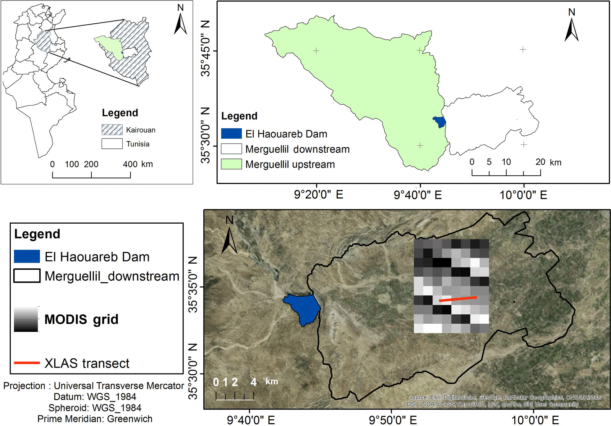
Figure 1The study area: the downstream Merguellil subbasin is the so-called Kairouan plain; the MODIS grid is the extracted 10 km × 8 km MODIS subimage and in red the scintillometer XLAS transect.
Contrarily to SWB models, most SEB models are run in their most standardized version, using observed RS-based parameters such as albedo in conjunction with a set of input parameters taken from literature or in situ data. However, the SEB model validation with enough data in space and time is difficult to achieve, due to the limited availability of high-resolution thermal images (Chirouze et al., 2014). Therefore, it is usually possible to evaluate SEB models results only at similar scale (km) to medium- or low-resolution images. Indeed, the pixel size of thermal remote sensing images, except for the scarce Landsat7 images (60 m), covers a range of 1000 m (Moderate Sensors Resolution Imaging Spectroradiometer MODIS), to 4000 m (Geostationary Operational Environmental Satellite GEOS). However, direct methods measuring sensible heat fluxes (eddy covariance for example) only provide point measurements with a footprint considerably smaller than a satellite pixel. Therefore, scintillometry techniques have emerged as one of the best tools aiming to quantify averaged fluxes over heterogeneous land surfaces (Brunsell et al., 2011). They provide area-averaged sensible heat flux over areas comparable to those observed by satellites (Hemakumara et al., 2003; Lagouarde et al., 2002). Scintillometry can provide sensible heat using different wavelengths (optical wavelength ranges), aperture sizes (15–30 cm) and configurations (long-path and short-path scintillometry) (Meijninger et al., 2002). The upwind area contributing to the flux (i.e., the flux footprint) varies as wind direction and atmospheric stability and must be estimated for the surface measurements in order to compare them to SEB estimates of the flux which are representative of the pixel (Brunsell et al., 2011). Assessing the upwind area contributing to the flux can be done using several footprint models (Schmid, 2002). Although footprint analysis ensures ad hoc spatial intersecting area between ground measurements and satellite-based surface fluxes, the spatial heterogeneity at subpixel scale should be further considered in validating low-resolution satellite data (Bai et al., 2015). The LAS technique has been validated over heterogeneous landscapes against eddy covariance measurements (Bai et al., 2009; Chehbouni et al., 2000; Hoedjes et al., 2009) and also against modeled fluxes (Marx et al., 2008; Samain et al., 2012; Watts et al., 2000). Few studies dealt with extra-large aperture scintillometer (XLAS) data (Kohsiek et al., 2002, 2006; Moene et al., 2006). Historical survey, theoretical background and recent works in applied research concerning scintillometry are reviewed in De Bruin and Wang (2017). Since the scintillometer provides large-scale area-average sensible heat flux (H_XLAS), the corresponding latent heat flux (LE_XLAS) can then be computed as the energy balance residual term (LE_XLAS = Rn − G − H_XLAS); hence, the estimation of a representative value for the available energy (AE = Rn − G) is always crucial for the accuracy of the retrieved values of LE_XLAS. This assumption is valid only under the similarity hypothesis of Monin–Obukhov (MO) (Monin and Obukhov, 1954), i.e., surface homogeneity and stationary flows. These hypotheses are verified in our study area where the topography is flat, and the landscape is heterogeneous only from an agronomic point of view since we find different land uses (cereals, market gardening and fruit trees, mainly olive trees with considerable spacing of bare soil); however, this heterogeneity in landscape features at field scale is randomly distributed and there is no drastic change in height and density of the vegetation at the scale of the XLAS transect (i.e., little heterogeneity at the kilometer scale, most MODIS pixels have similar NDVI values for instance).
In this study, spatially distributed estimates of surface energy fluxes (sensible heat H and latent heat fluxes LE) over an irrigated area located in the Kairouan plain (central Tunisia) were obtained by the SEB method, using the Soil Plant Atmosphere and Remote Sensing Evapotranspiration (SPARSE) model (Boulet et al., 2015) fed by 1 km thermal data and 1 km NDVI data from MODIS sensors on the Terra and Aqua satellites. The main objective of this paper is to compare the modeled H and LE simulated by the SPARSE model with, respectively, the H measured by the XLAS and the LE reconstructed from the XLAS measurements acquired in the course of 2 years over a large, heterogeneous area. We explore the consistency between the instantaneous H and LE estimates at the satellite overpass times, the water stress estimates and also ET derived at daily time steps from both approaches.
2.1 Study area
The study site is a semiarid region located in central Tunisia, the Kairouan plain (35∘1′–35∘55′ N, 9∘23′–10∘17′ E; Fig. 1). The landscape is mainly flat, and the vegetation is dominated by agricultural production (cereals, olive groves, fruit trees, market gardening; Zribi et al., 2011). Water management in the study area is typical of semiarid regions with an upstream subcatchment that transfers surface and subsurface flows collected by a dam (the El Haouareb dam) and a downstream plain (Kairouan plain) supporting irrigated agriculture (Fig. 1). Agriculture consumes more than 80% of the total amount of water extracted each year from the Kairouan aquifer (Poussin et al., 2008). Most farmers in the plain use their own wells to extract water for irrigation (Pradeleix et al., 2015), while a few depends on public irrigation schemes based on collective networks of water distribution pipelines all linked to a main borehole. The crop intensification in recent decades, associated with increasing irrigation, has led to growing water demand, and an over-exploitation of the groundwater (Leduc et al., 2004).
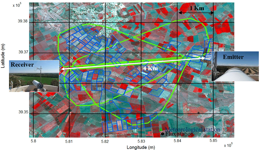
Figure 2XLAS setup: XLAS transect (white), for which the emitter and the receiver are located at the extremity of each white arrow; half-hourly XLAS footprint for selected typical wind conditions (green); MODIS grid (black); orchards (blue); and the location of the Ben Salem meteorological and flux stations. Background is a three-color (red, green, blue) composite of SPOT5 bands 3 (NIR), 2 (VIS-red) and 1 (VIS-green) acquired on 9 April 2013 and showing in red the cereal plots.
2.2 Experimental setup and remote sensing data
An optical Kipp & Zonen extra-large aperture scintillometer (XLAS) was operated continuously for more than 2 years (1 March 2013 to 3 June 2015) over a relatively flat terrain (maximum difference in elevation of about 18 m). The scintillometer consists of a transmitter and a receiver, both with an aperture diameter of 0.3 m, which allows longer path length. The wavelength of the light beam emitted by the transmitter is 940 nm. The transmitter was located on an eastern water tower (coordinates: 35∘34′0.7′′ N, 9∘53′25.19′′ E; 127 m a.s.l. – above sea level) and the receiver on a western water tower (coordinates: 35∘34′17.22′′ N, 9∘56′7.30′′ E; 145 m a.s.l.) separated by a path length of 4 km (Fig. 2).
The scintillometer transect was above a mixed-vegetation canopy: trees (mainly olive orchards) with some annual crops (cereals and market gardening) and the mean vegetation height is estimated to be about 1.17 m along the transect. Both instruments were installed at 20 m height as recommended in the Kipp & Zonen instruction manual for LAS and XLAS (Kipp & Zonen, 2017). At this height and for a 4 km path length, the devices are high enough to minimize measurement saturation and assumed to be above or close to the blending height where MO applied.
Furthermore, two automatic Campbell Scientific (Logan, USA) eddy covariance (EC) flux stations were also positioned at the same level on the two water-tower-top platforms. Half-hourly turbulent fluxes in the western and the eastern EC stations were measured using a sonic anemometer CSAT3 (Campbell Scientific, USA) at a rate of 20 Hz and a sonic anemometer RM 81000 (Young, USA) at a rate of 10 Hz, respectively. The western station data were more reliable with less measurement errors and gaps; hence, the western EC setup was used to initialize friction velocity u* values and the Obukhov length Lo in the scintillometer flux computation (Sect. 3.1).
Half-hourly standard meteorological measurements including incoming long wave radiation, i.e., global incoming radiation (), the incoming longwave radiation (i.e., atmospheric radiation, Ratm-30), wind speed (u30), wind direction (, air temperature (T30), relative humidity (RH30) and barometric pressure (P30) were recorded using an automated weather station installed in the study area (Fig. 2), referred to as the Ben Salem meteorological station (35∘33′1.44′′ N, 9∘55′18.11′′ E). Meteorological data were used either to force the SPARSE model or as input data in XLAS-derived sensible and latent heat flux. The global incoming radiation was also used in the extrapolation method to scale instantaneous observed (Sect. 3.3.2) and modeled (Sect. 4.2) available energy as well as modeled sensible heat flux (Sect. 4.2) to daily values.
In addition, an EC flux station, referred to as the Ben Salem flux station (a few tens of meters away from the meteorological station) was installed from November 2012 to June 2013 in an irrigated wheat field (Fig. 2) to measure half-hourly convective fluxes exchanged between the surface and the atmosphere (HBS-30 and LEBS-30) combined with measurements of the net radiation and the soil heat flux GBS-30. Net radiation and soil heat flux measurements were transferred to the meteorological station from June 2013 till June 2015. Since there are no Rn and G measurements in the two water towers EC stations, and GBS measurements were among the input data to derive sensible and latent heat fluxes from the XLAS measurements. In addition, measured available energy (AEBS = − GBS) and HBS were used to calibrate the extrapolation relationship of the available energy and the sensible heat flux, respectively (Sects. 3.3.2 and 4.2).
Remotely sensed data were acquired for the study period (1 September 2012 to 30 June 2015) at the resolution of the MODIS sensor at 1 km, embarked on board of the satellites Terra (overpass time around 10:30 local solar time) and Aqua (overpass time around 13:30 local solar time). Downloaded MODIS products were (i) MOD11A1 and MYD11A1 for Terra and Aqua, respectively (surface temperature Tsurf, surface emissivity εsurf and viewing angle ϕ); (ii) MOD13A2 and MYD13A2 for Terra and Aqua, respectively (NDVI); and (iii) MCD43B1, MCD43B2 and MCD43B3 (albedo α). These MODIS data provided in sinusoidal projection were reprojected in the Universal Transverse Mercator coordinate system using the MODIS Reprojection Tool. Then, subimages of 10 km × 8 km centered on the XLAS transect (Fig. 1) were extracted. The daily MODIS Tsurf and viewing angle, 8-day MODIS albedo, and 16-day MODIS NDVI contain some missing or unreliable data; hence, days with missing data (35 % of all dates) in MODIS pixels regarding the scintillometer footprint (see later footprint computation in Sect. 3.2) were excluded. Albedo products (MCD43) are available every 8 days; the day of interest is the central date. Both Terra and Aqua data are used in the generation of this product, providing the highest probability for quality input data and designating it as a combined product. Moreover, the 1 km and 16-day NDVI products (MOD13A2/MYD13A2) are available every 16 days and separately for Terra and Aqua. Algorithms generating this product operate on a per-pixel basis and require multiple daily observations to generate a composite NDVI value that will represent the full period (16 days). For both products, data are linearly interpolated over the available dates in order to get daily estimates. For each pixel, the quality index supplied with each product is used to select the best data.
3.1 Scintillometer-derived fluxes
Scintillometer measurements are based on the scintillation theory; fluxes of sensible heat and momentum cause atmospheric turbulence close to the ground, and create, with surface evaporation, refractive index fluctuations due mainly to air temperature and humidity fluctuations (Hill et al., 1980). The fluctuation intensity of the refractive index is directly linked to sensible and latent heat fluxes. The light beam emitted by the XLAS transmitter towards the receiver is dispersed by the atmospheric turbulence. The scintillations representing the intensity fluctuations are analyzed at the XLAS receiver and are expressed as the structure parameter of the refractive index of air integrated along the optical path (m) (Tatarskii, 1961). The sensitivity of the scintillometer to along the beam is not uniform and follows a bell-shaped curve due to the symmetry of the devices. This means that the measured flux is more sensitive to sources located towards the transect center and is less affected by those close to the transect extremities.
In order to compute the XLAS sensible heat flux, was converted to the structure parameter of temperature turbulence (K2 m) by introducing the Bowen ratio (ratio of sensible to latent heat fluxes), hereafter referred to as β, which is a temperature–humidity correlation factor. Moreover, the height of the scintillometer beam above the surface varies along the path. In our study site, the terrain is very flat leading to little beam height variation across the landscape, except for what is induced by the different roughness values of the individual fields. Since the interspaces between trees are large, the effective roughness of the orchards is not significantly different from that of annual crop fields. Consequently, and therefore are not only averaged horizontally but vertically as well.
At visible wavelengths, the refractive index is sensitive to temperature fluctuations. Then, we can relate the to as follows:
with T the air temperature (∘K) and P the atmospheric pressure (Pa).
Green and Hayashi (1998) proposed another method to compute XLAS sensible heat flux (H_XLAS) assuming full energy budget closure and using an iterative process without the need for β as an input parameter. This method is called the “β-closure method” (BCM, Twine et al., 2000). In the calculation algorithm, β is estimated iteratively with the BCM method, as described in Solignac et al. (2009) with an initial guess using and GBS from the Ben Salem flux station and initial u* coming from the western water tower EC station.
Then, the similarity relationship proposed by Andreas (1988) is used to relate the to the temperature scale T* in unstable atmospheric conditions as follows:
and for stable atmospheric conditions,
where LO (m) is the Monin–Obukhov length, ZLAS (m) is the scintillometer height, and d (m) is the displacement height, which corresponds to two-thirds of the averaged vegetation height zv.
The variable zv counts for the various heights within the selected footprint using angular zones originating from the center of the transect and supported by high-resolution remote sensing data (see Sect. 4.1).
Furthermore, considering the size of the surface changes in roughness (mean or effective vegetation height ∼ 1.5 m), the XLAS measurement height is assumed to be either close to the blending height or higher. Thus, the fluxes measured by XLAS are area-averaged and the MO similarity hypothesis can be applied in the flux algorithm computation.
Moreover, the fluxes measured with the XLAS were calculated for a stability index (ZLAS∕LO) between −2 and 0 (∼ 73 % of the cases). Then, according to Gruber and Fochesatto (2013), the sensitivity of the turbulent flux measurements to uncertainties in source measurements is rather similar between iterative algorithms and analytical solution, in this range of atmospheric stability.
From T* and the friction velocity u* (computed based on an iteration approach in the BCM method), the sensible heat flux can be derived as follows:
where ρ (kg m−3) the density of air and cp (J kg−1 K−1) the specific heat of air at constant pressure.
H_XLAS was computed at a half-hourly time step. Before flux computation, a strict filtering was applied to the XLAS data to remove outliers depending on weak demodulation signal. Negative nighttime data were set to zero and daytime flux missing data (one to three 30 min data) were gap filled using simple interpolation. Furthermore, half-hourly H_XLAS aberrant values due to measurement errors and values higher than 400 W m−2, arising from measurement saturation, were ruled out (3 % of the total measurement throughout the experiment duration). Finally, daily H_XLAS was computed as the average of the half-hourly H_XLAS.
3.2 XLAS footprint computation
The footprint of a flux measurement defines the spatial context of the measurement and the source area that influences the sensors. In case of inhomogeneous surfaces like patches of various land covers and moisture variability due to irrigation, the measured signal is dependent on the fraction of the surface having the strongest influence on the sensor and thus on the footprint size and location. Footprint models (Horst and Weil, 1992; Leclerc and Thurtell, 1990) have been developed to determine what area is contributing to the heat fluxes as well as the relative weight of each particular cell inside the footprint limits. Contributions of upwind locations to the measured flux depend on the height of the vegetation, height of the instrumentation, wind speed, wind direction and atmospheric stability conditions (Chávez et al., 2005).
According to the model of Horst and Weil (1992), for a one-point measurement system, the footprint function f relates the spatial distribution of surface fluxes, F0(x, y), to the measured flux at height, zm, F(x, y, zm), as follows:
The footprint function f is computed as follows:
where is the mean wind speed profile and is the mean plume height for diffusion from a surface source. The variables A, b and c are scale factors and r is a scale factor of the Gamma function. In the case of a scintillometer measurement, the footprint function has to be combined with the spatial weighting function W(x) of the scintillometer to account for the sensor integration along its path. Thus, the sensible heat flux footprint mainly depends on the scintillometer effective height ZLAS (Hartogensis et al., 2003), which includes the topography below the path and the transmitter and receiver heights, the wind direction, and the Obukhov length LO, which characterizes the atmospheric stability (Solignac et al., 2009). In a subsequent step, daily footprints were computed as a weighted sum of the half-hourly footprints by the XLAS sensible heat flux.
In fact, there is an issue with the MODIS pixel heterogeneity and notably the distribution of the land use classes at the intersection between the square pixel and the XLAS footprint (Bai et al., 2015). Hence, in order to provide a first guess on these relative heterogeneities, land use classes within each MODIS pixel of the 10 km × 8 km subimage were studied based on the land use map of the 2013–2014 season (Chahbi et al., 2016). The average footprint of all half-hourly footprints for the whole study period was computed and overlaid on the MODIS grid in order to identify the MODIS pixels partially or totally covered by footprint (Fig. 3).
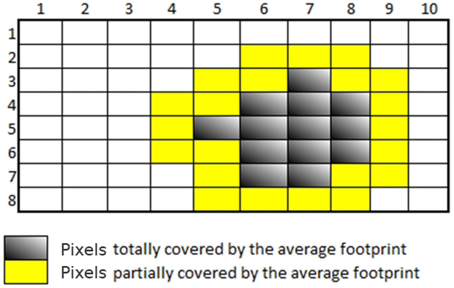
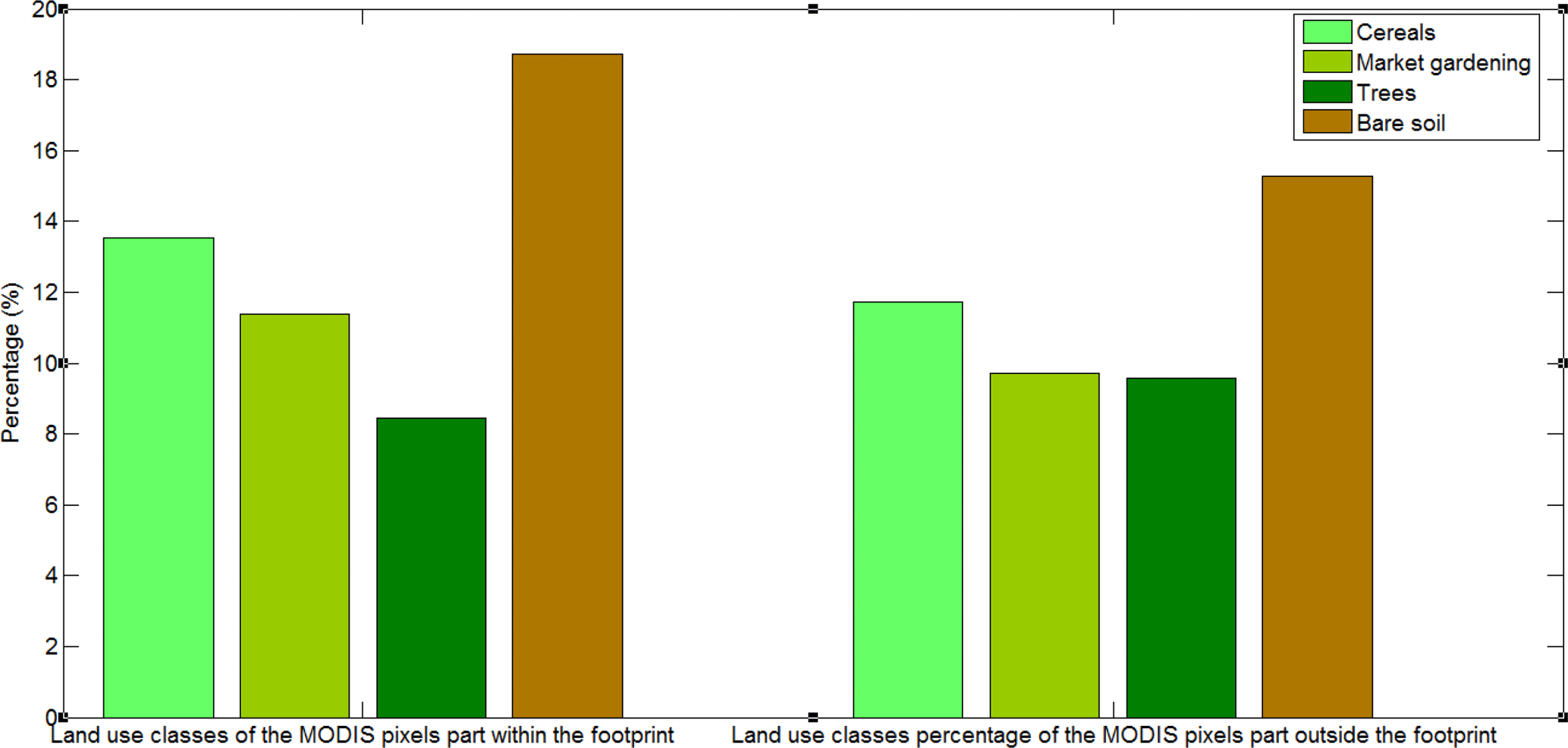
The percentage of land use classes was computed for (i) the part of each pixel that lies within the footprint and (ii) the complementary part of the pixel located outside of the footprint (Fig. 4). Results show that differences in percentages of each land use classes for the pixel fractions located within or outside the footprint are low, with 1.8, 1.7, 1.0 and 3.5 % for cereals, market gardening, trees and bare soil, respectively. Moreover, the major part of the area above the transect is covered by fallow and orchards. The land use classes' partition inside the 13 MODIS pixels totally covered by the average footprint is comparable.
3.3 XLAS-derived latent heat flux
Instantaneous (LE_residual_XLASt-FP) and daily (LE_residual_XLASday-FP) XLAS-derived latent heat fluxes (i.e., residual latent heat flux) of the XLAS upwind area were computed using the energy budget closure of the XLAS measured sensible heat flux (H_XLAS) with additional estimations of remotely sensed net surface radiation Rn and soil heat flux G, as available energy (AE = Rn − G), as follows:
H_XLASt and H_XLASday are respectively the instantaneous and daily measured H at the times of the satellite overpass interpolated from the half-hourly fluxes measurements. Daily available energy within the footprint (AEday-FP) was computed from instantaneous available energy (AEt-FP) as detailed in Sect. 3.3.1 and Sect. 3.3.2. The subscripts “30”, “day” and “t” refer to half-hourly, daily and instantaneous (at the times of Terra and Aqua overpasses) variables, respectively, while the subscript “FP” means that the footprint is taken into account, i.e., instantaneous or the daily (depending on timescale) footprint was multiplied by the variable.
3.3.1 Instantaneous available energy
Net surface radiation is the balance of energy between incoming and outgoing shortwave and longwave radiation fluxes at the land–atmosphere interface. Remotely sensed surface radiative budget components provide unparalleled spatial and temporal information, and thus several studies have attempted to estimate net radiation by combining remote sensing observations with surface and atmospheric data. Net radiation equation can be written as follows:
where Rg is the incoming shortwave radiation (W m−2), Ratm is the
incoming longwave radiation (W m−2), α is the albedo,
Tsurf is the surface emissivity, εsurf is the surface temperature (∘K)
and σ is the Stefan–Boltzmann constant (W−2 K4). The soil heat
flux G depends on the soil type and water content as well as the vegetation
type (Allen et al., 2005). The direct estimation of G by remote sensing data
is not possible (Allen et al., 2011); however, empirical relations can
estimate the fraction ξ = G∕Rn as a function of soil and vegetation
characteristics using satellite image data, such as the LAI, NDVI,
α and Tsurf. Generally, G represents 5–20 % of Rn during daylight hours
(Kalma et al., 2008). In order to estimate the G∕Rn ratio, several methods
have been tested for various types of surfaces at different locations. The
most common methods parameterize ξ as a constant for the entire day or
at satellite overpass time (Ventura et al., 1999), according to NDVI
(Jackson et al., 1987; Kustas and Daughtry, 1990), LAI
(Choudhury et al., 1987; Kustas et al., 1993; Tasumi et al., 2005),
vegetation fraction (fc) (Su, 2002), Tsurf and α
(Bastiaanssen, 1995), or only Tsurf (Santanello Jr. and Friedl,
2003). These empirical methods are suitable for specific conditions;
therefore, estimating G, especially in this type of environment where NDVI
values are low and thus G∕Rn values are large, is a critical issue. The
approach adopted here was drawn on Danelichen et al. (2014), who
evaluated the parameterization of these different models in three sites in
Mato Grosso state in Brazil and found that the model proposed by
Bastiaanssen (1995) showed the best performance for all sites, followed
by the model from Choudhury et al. (1987) and Jackson et al. (1987):
Bastiaanssen (1995):
Choudhury et al. (1987):
Jackson et al. (1987)
Hence, these three methods were tested for the Ben Salem flux station measurements, by comparing the measured GBS-t and the computed G using measured , Tsurf-BS-t, αBS, NDVIBS and LAIBS at Terra and Aqua overpass times (results not shown). The best results are issued from the Bastiaanssen (1995) method with a root mean square error (RMSE) of 0.09 (average value of the two satellite overpass times) followed by Jackson et al. (1987) and Choudhury et al. (1987) with RMSE values of 0.15 and 0.2, respectively. Moreover, daily measured GBS-day was computed and a G accumulation is generally found as has been already mentioned by Clothier et al. (1986), who showed that G is neither constant nor negligible on diurnal timescales and can constitute as much as 50 % of Rn over sparsely vegetated area. Since G estimation was the most uncertain variable, the three above methods were tested to compute the distributed remotely sensed AE. The Ben Salem meteorological station was used to provide and Ratm-t. Remote sensing variables α, Tsurf, εsurf and NDVI came from MODIS products. Remotely sensed LAI was computed from the MODIS NDVI using a single equation (Clevers, 1989) for all crops in the study area:
The calibration of this relationship was done over the Yaqui irrigated perimeter (Mexico) during the 2007–2008 growing season using hemispherical LAI measured in all the studied fields (Chirouze et al., 2014). Calibration results gave the asymptotical values of NDVI, NDVI∞ = 0.97 and NDVIsoil = 0.05, as well as the extinction factor k = 1.13. As this relationship was calibrated over a heterogeneous land surface but on herbaceous vegetation only, its relevance for trees was checked. For that purpose, clump-LAI measurements on an olive tree, as well as allometric measurements, i.e., mean distance between trees and mean crown size done using Pleiades satellite data (Mougenot et al., 2014; Touhami, 2013) were obtained. Clump LAI is the value of the LAI of an isolated element of vegetation (tree, shrub, etc.); if this element occupies a fraction cover f and is surrounded by bare soil, then the clump LAI value is equal to the area-average LAI divided by f. Hence, we checked that the pixels with tree-dominant cover show LAI values close to what was expected (of the order of 0.3 to 0.4 given the interrow distance of 12 m on average).
Remote sensed available energy was computed for the 10 km × 8 km MODIS subimages at Terra MODIS and Aqua MODIS overpass times, using the three methods estimating G. Since the measured heat fluxes H_XLASt represent only the weighted contribution of the fluxes from the upwind area to the tower (footprint), then instantaneous footprints at the times of Terra and Aqua overpass were selected among the two half-hours preceding and following the satellite's time of overpass (lowest time interval) and then was multiplied by the instantaneous remotely sensed available energy AEt to get the available energy of the upwind area AEt-FP.
3.3.2 Daily available energy
Most methods using TIR domain data rely on once-a-day, late morning (such as Terra-MODIS overpass time) or early afternoon (such as Aqua-MODIS overpass time) acquisitions. Thus, they provide a single instantaneous estimate of energy budget components. In order to obtain daily AE from these instantaneous measurements and to reconstruct hourly variations of AE, we considered that its evolution was proportional to another variable whose diurnal evolution can be easily known.
The extrapolation from an instantaneous flux estimate to a daytime flux assumes that the surface energy budget is “self-preserving”, i.e., the relative partitioning among components of the budget remains constant throughout the day. However, many studies (Brutsaert and Sugita, 1992; Gurney and Hsu, 1990; Sugita and Brutsaert, 1990) showed that the self-preservation method gives daytime latent heat estimates that are smaller than observed values by 5–10 %. Moreover, Anderson et al. (1997) found that the evaporative fraction computed from instantaneous measured fluxes tends to underestimate the daytime average by about 10 %; hence, a corrected parameterization was used and a coefficient = 1.1 was applied. Similarly, Delogu et al. (2012) found an overestimation of about 10 % between estimated and measured daily components of the available energy, and thus a coefficient = 0.9 was applied. The corrected parameterization proposed by Delogu et al. (2012) was tested, but this coefficient did not give consistent results; therefore, the extrapolation relationship was calibrated in order to get accurate daily results of AE.
Thereby, the applied extrapolation method was tested using in situ Ben Salem flux station measurements. The incoming short-wavelength radiation was used to scale available energy from instantaneous to daily values, but only for clear-sky days for which MODIS images can be acquired and remote sensing data used to compute AE are available. Clear-sky days were selected based on the ratio of daily measured incoming short-wavelength radiation to the theoretical clear-sky radiation Rso as proposed by the FAO-56 method (Allen et al., 1998). A day was defined as clear if the measured is higher than 85 % of the theoretical clear-sky radiation at the satellite overpass times (Delogu et al., 2012).
Daily measured available energy AEBS-day, computed as the average of half-hourly measured AEBS-30, was compared to daily available energy (AEBS-day-Terra and AEBS-day-Aqua) computed using the extrapolation method from instantaneous measured AEBS-t-Terra and AEBS-t-Aqua at Terra and Aqua overpass times, respectively (Eq. 14).
where is the daily measured incoming short-wavelength radiation in the Ben Salem meteorological station; and are the instantaneous incoming short-wavelength radiation measured at Terra and Aqua overpass time, respectively, and AEBS-t-Terra and AEBS-t-Aqua are the instantaneous measured available energy in the Ben Salem flux station, at Terra and Aqua overpass times.
Results gave an overestimation of about 15 %. The corrected parameterizations of AE (Table 1), needed to remove the bias between measured (AEBS-day) and computed AE (AEBS-day-Terra and AEBS-day-Aqua), were applied to compute daily remotely sensed AE (AEday) from instantaneous AE (AEt) following the extrapolation method shown in Eq. (14).
Then AEday was multiplied by the corresponding daily footprint to get the daily available energy of the upwind area AEday-FP. Finally, estimates of Terra and Aqua observed daily LE (LE_residual_XLASday-FP) were obtained based on the three methods used to compute G.
4.1 Energy fluxes derived from SPARSE model
The SPARSE dual-source model solves the energy budgets of the soil and the vegetation. Here we use the “layer approach”, for which the resistance network relating the soil and vegetation heat sources to a main reference level through a common aerodynamic level use a series electrical branching. The main unknowns are the component temperatures, i.e., soil (Ts) and vegetation (Tv) temperatures. Totals at the reference height (the measurement height of the meteorological forcing), as well as the longwave radiation budget, are also solved so that altogether a system of five equations can be built:
where Ratm is the atmospheric radiation (W m−2), Ran is net longwave radiation which depends on Ts and Tv (W m−2), and Tsurf and εsurf are respectively the surface temperature (∘K) and emissivity as observed by the satellite; indexes “s” and “v” designate the soil and the vegetation, respectively.
The first two (Eq. 15) express the continuity of the latent and sensible heat fluxes from the sources to the aerodynamic level through to the reference level, the third and the fourth (Eq. 15) are the soil and vegetation energy budgets, and the fifth (Eq. 15) relates the surface temperature Tsurf derived from observed MODIS surface temperature to Ts and Tv.
Table 1Corrected parameterizations of available energy for the diurnal reconstitution.
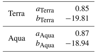
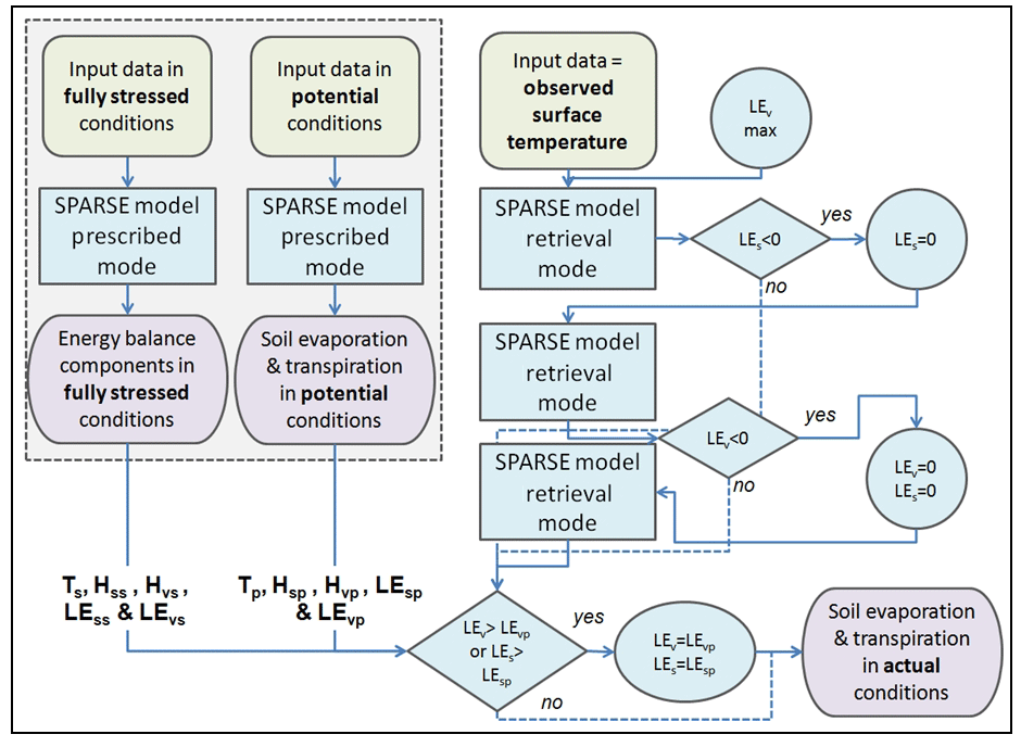
Figure 5Flowchart of the SPARSE algorithm; Ts, Hss, Hvs, LEss and LEvs are surface temperature, soil sensible heat flux, vegetation sensible heat flux, soil latent heat flux and vegetation latent heat flux in fully stressed conditions, respectively; Tp, Hsp, Hvp, LEsp and LEvp are surface temperature, soil sensible heat flux, vegetation sensible heat flux, soil latent heat flux and vegetation latent heat flux in potential conditions, respectively.
The SPARSE model system of equations is fully described in Boulet et al. (2015). SPARSE is similar to the TSEB model (Kustas and Norman, 1999) but includes the expressions of the aerodynamic resistances of Choudhury and Monteith (1988) and Shuttleworth and Gurney (1990). This system can be solved in a forward mode for which the surface temperature is an output (prescribed conditions), and an inverse mode when the surface temperature is an input derived from satellite observations or in situ measurements in the thermal infrared domain (retrieval conditions). Figure 5 illustrates a diagram showing the flowchart of the model algorithm. System (15) is solved step by step by following similar guidelines as in the TSEB model: the first step assumes that the vegetation transpiration (LEv) is at its maximum, and evaporation (LEs) is computed. If this soil latent heat flux (LEs) is below a minimum positive threshold for vegetation stress detection of 30 W m−2, the hypothesis that the vegetation is unstressed is no longer valid. In that case, the vegetation is assumed to suffer from water stress and the soil surface is assumed to be already long dry. Then, LEs is set to 30 W m−2. This value accounts for the small but nonnegligible vapor flow reaching the surface (Boulet et al., 1997). The system is then solved for vegetation latent heat flux (LEv). If LEv is also negative, both LEs and LEv values are set to zero, whatever the value of Tsurf. The system of equation can also be solved for Ts and Tv only if the efficiencies representing stress levels (dependent on surface soil moisture for the evaporation, and root zone soil moisture for the transpiration) are known. In that case the sole first four equations are solved. This prescribed mode allows all the fluxes in known limiting soil moisture levels to be computed (very dry, e.g., fully stressed, and wet enough, e.g., potential). It limits unrealistically high values of component fluxes, latent heat flux values above the potential rates or sensible heat flux values above that of a nonevaporating surface. The potential evaporation and transpiration rates used later on are computed using this prescribed mode with minimum surface resistance to evaporation and transpiration, respectively.
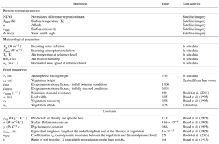
Some of the model parameters were remotely sensed data while others were taken from the bibliography or measured in situ. Remotely sensed data fed into SPARSE are Tsurf, εsurf, ϕ, NDVI, LAI and α. A grid of the vegetation height (zv) was also necessary as input in the SPARSE model; for herbaceous crops, vegetation height was interpolated with the help of NDVI time series between fixed minimum (0.05 m) and maximum (0.8 m) values, while for trees, the roughness length (zom) was linked to the allometric measurements (mentioned before) and computed as a function of canopy area index, drag coefficient and canopy height using the drag partition approach proposed by Raupach (1994) for tall sparse vegetative environments. Then, since SPARSE deals with vegetation height and not roughness length, the same simple rule of the thumb as the one used in SPARSE was used to reconstruct zv for the tree cover types (zv = zom∕0.13). In a final step, to get spatial vegetation height, zv was averaged over the MODIS pixels. In situ parameters used in SPARSE were mainly meteorological data: Rg, Ratm, Ta, Ha and u. No calibration was performed on the model parameters shown in Table 2.
The retrieval and prescribed modes of the SPARSE model were run for the 10 km × 8 km subimages at the times of Terra and Aqua overpasses, to get instantaneous modeled fluxes H_SPARSEt, LE_SPARSEt and AE_SPARSEt as well as sensible heat flux (Hs-t = Hss-t + Hvs-t) in fully stressed conditions and latent heat (LEp-t = LEsp-t + LEvp-t) and sensible heat (Hp-t = Hsp-t + Hvp-t) fluxes in potential conditions. Modeled values were then multiplied by the nearest half-hourly footprint to the satellite overpass time, in order to get fluxes corresponding to the upwind area: H_SPARSEt-FP, LE_SPARSEt-FP, AE_SPARSEt-FP, Hs-t-FP, Hp-t-FP and LEp-t-FP.
In a subsequent step, the retrieval and prescribed modes of SPARSE model was run at a half-hourly time step using the half-hourly meteorological measurements to get half-hourly latent heat flux at potential conditions LEp-30 and half-hourly modeled available energy AE_SPARSE30. The potential LE weighted by the corresponding half-hourly footprint (LEp-30-FP) is used later when computing daily LE based on the stress factor method, while the half-hourly AE weighted by the corresponding half-hourly footprint (AE_SPARSE30-FP) is used to compute daily LE based on the evaporative fraction method (Sect. 4.2).
4.2 Reconstruction of daily modeled ET from instantaneous latent heat flux
Daily ET is usually required for applications in hydrology or agronomy for instance, whereas most SEB methods provide a single instantaneous latent heat flux because the energy budget is only computed at the satellite overpass times (Delogu et al., 2012). In order to scale daily ET from one instantaneous estimate, there are various methods relying on the preservation, during the day, of the ratio of the latent heat flux to a scale factor with known diurnal evolution.
4.2.1 Stress factor (SF) method
The stress factor SF (Eq. 16) is assumed to be invariant during the same day, and the diurnal modeled fluxes are accounted for by recovering the diurnal course of potential ET.
The daily modeled ET (LE_SPARSEday-FP) can be expressed as the product of the instantaneous estimate of SF at the satellite overpass times and the daily potential evapotranspiration:
LEp-day-FP was calculated as the sum of the half-hourly modeled latent heat fluxes at potential conditions LEp-30-FP.
4.2.2 Evaporative fraction method
The evaporative fraction (EF) self-preservation is a valid assumption under dry conditions but no longer under wet conditions (Hoedjes et al., 2008). For these conditions, assuming a constant EF underestimates actual EF and therefore ET (Lhomme and Elguero, 1999). Indeed, according to Gentine et al. (2007), the diurnal shape of EF depends on both atmospheric forcing and surface conditions. Therefore EF was computed every 30 min using the following empirical parameterization (Delogu et al., 2012):
where and RH30 are respectively the half-hourly incoming short-wavelength radiation and relative humidity EFSPARSE-t and EFmet-t are respectively SPARSE EF (Eq. 19) and computed EF using the evaporative fraction method (Eq. 20) at the satellite overpass times.
where LE_SPARSEt-FP and AE_SPARSEt-FP are respectively the latent heat flux and the available energy modeled by SPARSE at the satellite overpass times; and RHt are respectively the incoming short-wavelength radiation and relative humidity measured at the times of the satellite overpasses.
The half-hourly modeled ET (LE_SPARSE30-FP) was computed as the product of the half-hourly EF estimate and the half-hourly modeled available energy AE_SPARSE30-FP (Eq. 21). AE_SPARSE30 was computed from instantaneous modeled available energy (AE_SPARSEt) using the same approach detailed in Sect. 3.3.2 and applying Eq. (14) for a half-hourly time step (instead of a daily time step). AE_SPARSE30 was weighted by the corresponding half-hourly footprint to get the modeled AE of the upwind area AE_SPARSE30-FP. The daily modeled ET (LE_SPARSEday-FP) was computed as the sum of the half-hourly LE_SPARSE30-FP (Eq. 22).
4.2.3 Residual method
Besides, daily modeled ET (LE_SPARSEday-FP) was also estimated as a residual term of the surface energy budget using daily modeled sensible heat flux (H_SPARSEday-FP) and available energy (AE_SPARSEday-FP) as follows:
H_SPARSEday was computed from modeled sensible heat flux (H_SPARSEt) following the same extrapolation method used for the available energy (see Sect. 3.3.2). The corrected parameterizations of H were obtained from the comparison of daily measured sensible heat flux HBS-day computed as the average of half-hourly measured HBS-30 and daily sensible heat flux (HBS-day-Terra and HBS-day-Aqua) computed using the extrapolation method from instantaneous measured HBS-t-Terra and HBS-t-Aqua at Terra and Aqua overpass times, respectively (Eq. 24).
where HBS-t-Terra and HBS-t-Aqua are the instantaneous measured sensible heat flux in the Ben Salem flux station.
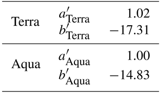
Therefore, the corrected parameterizations of H (Table 3), needed to remove the bias between measured (HBS-day) and computed H (HBS-day-Terra and AEBS-day-Aqua), were applied to compute daily modeled H (H_SPARSEday) from instantaneous modeled H (H_SPARSEt) following the extrapolation method shown in Eq. (21). Finally, H_SPARSEday was weighted by the corresponding daily footprint to get the daily modeled H of the upwind area H_SPARSEday-FP.
Table 3Corrected parameterizations of sensible heat flux for the diurnal reconstitution.
Water stress estimation is crucial to deduce the root zone soil moisture level using remote sensing data (Hain et al., 2009). Water stress results in a drop of actual evapotranspiration below the potential rate. Its intensity is usually represented by a stress factor as defined in Sect. 4.2, ranging between 0 (unstressed surface) and 1 (fully stressed surface).
Modeled values of SF at the times of Terra and Aqua overpasses (SFmod) have been computed from modeled potential LE (LEp-t-FP) as follows:
where LE_SPARSEt-FP and LEp-t-FP are the modeled latent heat fluxes in actual and potential conditions, respectively.
Furthermore, surface water stress factor derived from XLAS measurement, named SFobs, at the times of Terra and Aqua overpasses was computed as follows (Su, 2002):
where Hs-t-FP and Hp-t-FP are the modeled sensible heat flux in actual and potential conditions, respectively, and H_XLASt is the XLAS sensible heat flux at the satellite overpass times.
6.1 XLAS- and model-derived instantaneous sensible heat fluxes
Our primary focus is the comparison between scintillometer measurements and the modeled sensible heat fluxes computed using the Terra and Aqua remotely sensed data. The scintillometer H at the times of the two satellite overpasses (H_XLASt) are interpolated from the half-hourly H measurements. Heat flux determination was possible for typically about 87 % of the daytime measurements during the summer, availability of XLAS heat flux values was lower during the cold season due to poor visibility and/or stable stratification.
H_SPARSE was weighted by the XLAS footprint in order to be able to compare the modeled values (H_SPARSEt-FP) with the XLAS measurements (H_XLASt). Therefore, due to XLAS and remote sensing data availability, we got 175 and 118 values for Terra and Aqua respectively. In order to highlight H interseasonality between the drier 2012–2013 and the wetter 2013–2014 seasons, we present an example of 2 days, each in one season: DOY 2013-082 shows a H value ranging between 163 and 342 W m−2 while DOY 2014-208 shows a H value ranging between 97 and 311 W m−2 (Fig. 6). The colored area shows the modeled flux and the contours shows the surface source area contributing to the scintillometer measurements. Day 2013-82 (23 March 2013) is chosen in the cold season while day 208-2014 (27 July 2014) is in the warm season to focus on land cover impact on Tsurf and thus on modeled H (trees and cereals in winter vs. only irrigated trees and market gardening in summer). Moreover, the first day experiences a strong southern wind while there is a light northern wind during the second day. Generally, a small number of MODIS pixels brings a high contribution to the signal; among these, two are hot pixels (pixel with high Tsurf and low NDVI) in which the land use is mainly arboriculture.
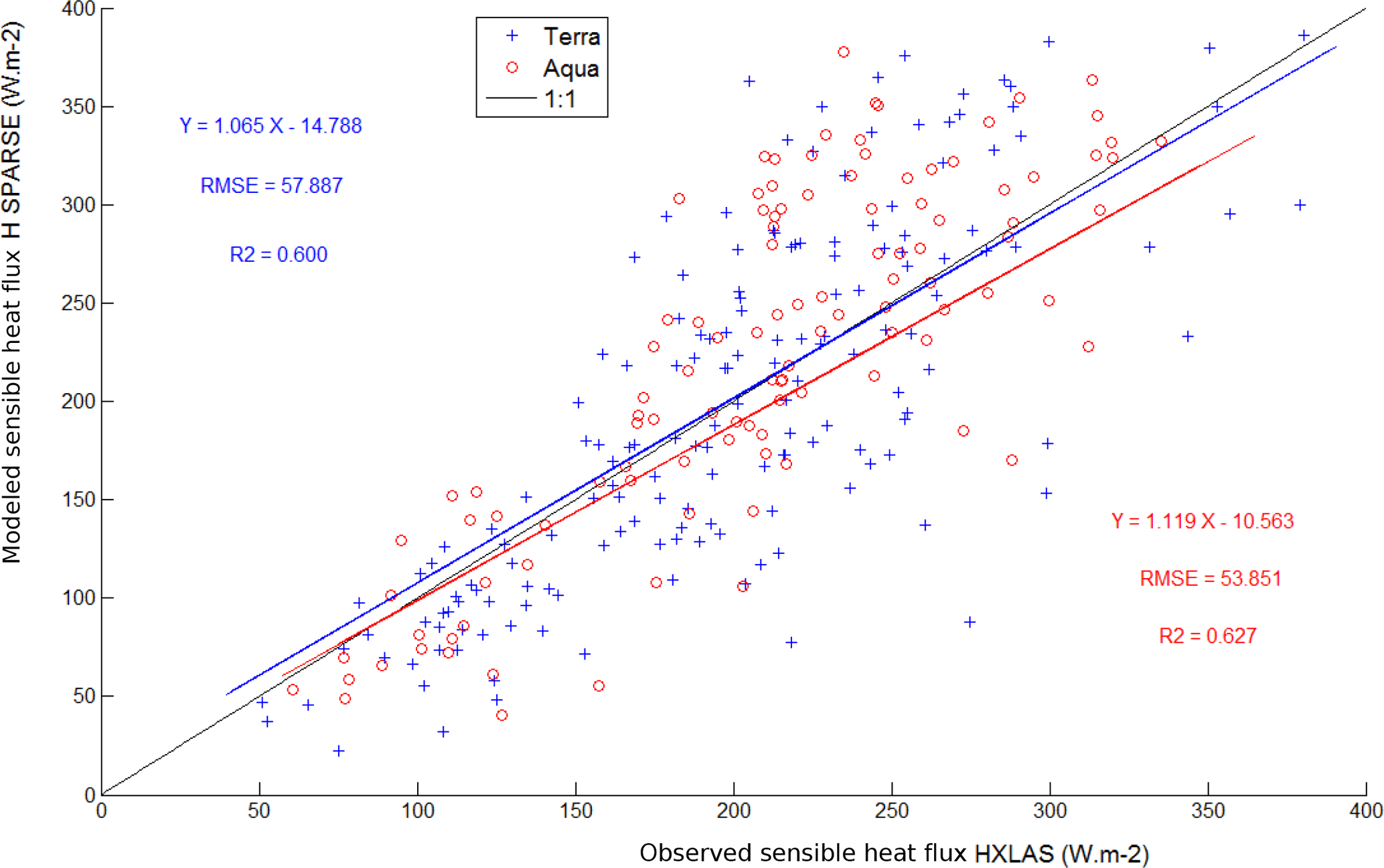
Prediction performance is assessed using RMSE and the coefficient of determination (R2). Results for the sensible heat flux are illustrated in Fig. 7 and show good agreement between modeled and measured H at the times of satellite overpasses. This is illustrated by linear regressions of H_SPARSEt-FP = 1.065 H_XLASt − 14.788 (R2 = 0.6; RMSE = 57.89 W m−2) and H_SPARSEt-FP = 1.12 H_XLASt − 10.57 (R2 = 0.63; RMSE = 53.85 W m−2) for Terra and Aqua, respectively. This result is of great interest considering that the SPARSE model was run with no prior calibration. However, we noted that bias is a function of the flux level and most outliers are recorded for H greater than 200 W m−2. This can be explained by (i) the XLAS measurement saturation (according to the “Kipp & Zonen LAS and XLAS instruction manual” (Kipp & Zonen, 2017), for a path length of 4 km and a scintillometer height of 20 m, the saturation measurement problems start from H values higher than 300 W m−2), (ii) uncertainties on the correction of stability using the universal stability function, and (iii) potential inconsistencies between the area average MODIS surface temperature and the air temperature measured locally at the meteorological station.
Whereas there are several studies dealing with large aperture scintillometer data whose measurements are compared to modeled fluxes, in the few studies dealing with extra large aperture scintillometer data, the comparison is generally done with eddy covariance station measurements (Kohsiek et al., 2002; Moene et al., 2006). Indeed, our results are in agreement with those found by Marx et al. (2008), who compared LAS-derived and satellite-derived H (SEBAL was applied with NOAA-AVHRR images providing maps of surface energy fluxes at a 1 km × 1 km spatial resolution) and found that modeled H is underestimated with a RMSE of 39 W m−2 for the site Tamale and 104 W m−2 for the site Ejura. Moreover, Watts et al. (2000) compared the satellite (AVHRR radiometer) estimates of H to those from LAS over semiarid grassland in north-western Mexico during the summer of 1997. They found RMSE values of 31 and 43 W m−2 for LAS path lengths of 300 m and 600 m respectively and showed that LAS measurements are less good than those derived from a 3-D sonic anemometer. They also suggested longer LAS path length (greater than 1.1 km) since the LAS is rather insensitive to the surface near the receiver and the emitter.
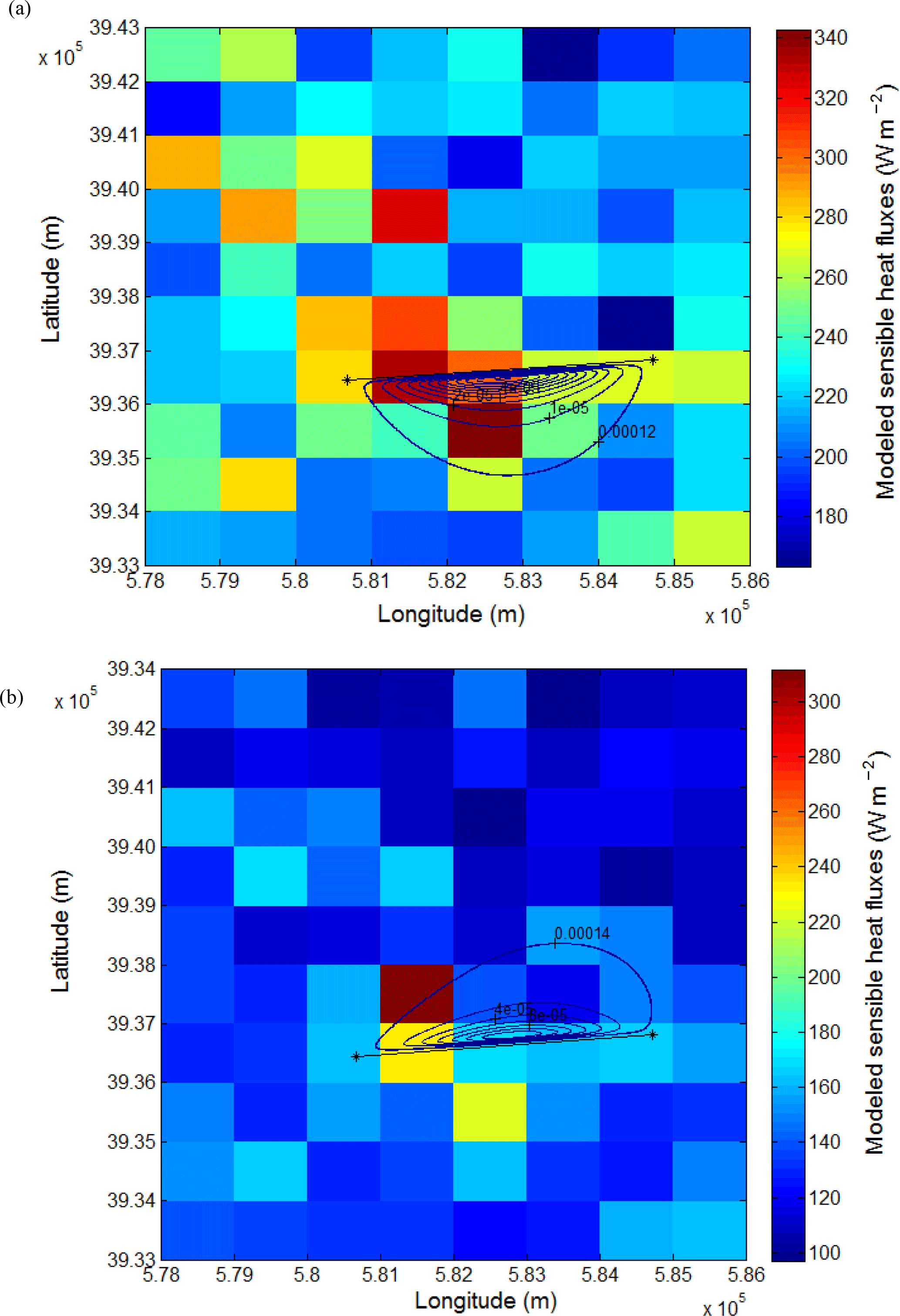
Figure 6Model-derived sensible heat fluxes and footprints for (a) DOY 2013-082 at Aqua overpass time and (b) DOY 2014-208 at Terra overpass time. The colored area shows the modeled flux and the contours shows the surface source area contributing to the scintillometer measurements.
6.2 XLAS- and model-derived instantaneous latent heat fluxes
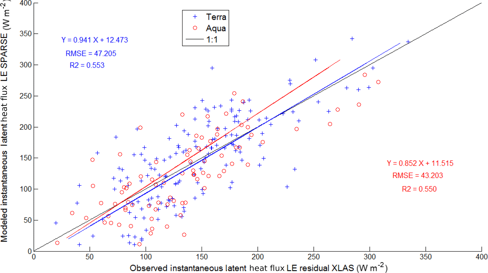
In a subsequent step, SPARSE-derived LE (LE_SPARSEt-FP) was compared to observed LE (LE_residual_XLASt-FP). Results are illustrated in Fig. 8, showing a good agreement between modeled and observed LE. However, these results are less good than for the H results, as shown by the following linear regressions: LE_SPARSEt-FP = 0.94 LE_residual_XLASt-FP + 12.47 (RMSE = 47.20 W m−2) and LE_SPARSEt-FP = 0.85 LE_residual_XLASt-FP + 11.51 (RMSE = 43.20 W m−2) for Terra and Aqua respectively, with an overall R2 of 0.55 for both satellites. We note a greater scatter for latent heat flux than for the sensible heat flux (Fig. 7), which can be explained by the fact that LE is here a residual term affected by estimation errors in both AE and H. Despite this moderate discrepancy, the good agreement between both approaches indicates that the methodology adopted in SPARSE for estimating H and AE using MODIS imagery is appropriate for modeling latent heat fluxes.
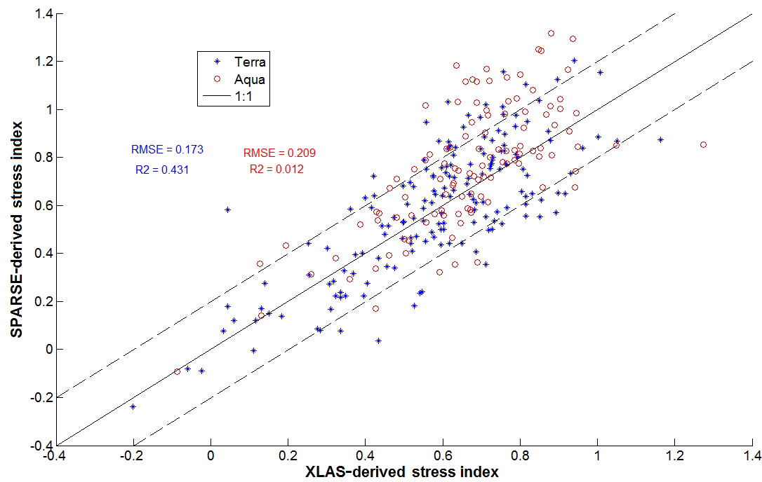
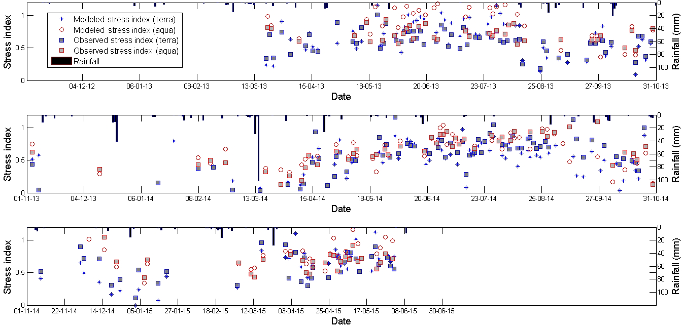
Figure 10Modeled and observed stress index evolution at Terra and Aqua overpass times compared to daily rainfall.
6.3 Water stress
The scattered values of the stress factor as shown in Fig. 9 are consistent with previous studies such as Boulet et al. (2015). SEB retrieval of stress is limited by the scale mismatch between the instantaneous estimate of the surface temperature during the satellite overpass (which can be influenced by high-frequency turbulence) and the aggregated values of other forcing data which are derived from half-hourly averages (Lagouarde et al., 2013, 2015). However, general tendencies are well reproduced, with most points located within a 0.2 confidence interval (illustrated by dotted lines along the 1 : 1 line) as found by Boulet et al. (2015) at field scale, which is encouraging from the perspective of assimilating ET or SF in a water balance model for example. Moreover, it is noted that results include small LE and LEp values with the same order of magnitude as the measurement uncertainty itself. Most outliers with greater water stress (∼ 1) correspond to high evaporation from bare soil since the dominant land use in the study area is arboriculture, but also, this could be due to saturation of scintillation which led to an underestimation of H XLAS measurements, as pointed out by Frehlich and Ochs (1990) and Kohsiek et al. (2002).

Figure 11Modeled vs. observed daily latent heat fluxes. Dark grey color shows minimum and maximum daily observed LE. Light grey vertical bars show gaps in XLAS data. Error bars for the modeled ET show the minimum and the maximum daily ET resulting from the three methods used to compute daily ET from instantaneous modeled ET.
Modeled and observed stress indexes at Terra and Aqua overpass times show a consistent evolution with daily rainfall (Fig. 10), although the modeled stress shows a greater dispersion than the observed one. During a rainy episode (or an eventual irrigation period), the surface temperature decreases towards the unstressed surface temperature, thus marking an unstressed state, and SF tends to 0. Conversely, after a long dry down, the water stress appears and the surface temperature increases towards the equilibrium surface temperature computed by SPARSE under stressed conditions, and SF tends towards 1. Besides, it is noted that modeled stress indexes computed on the basis of Aqua MODIS's Tsurf are often greater than those computed using Terra MODIS's Tsurf due to higher Tsurf (higher global solar radiation) at the time of Terra overpass (around midday).
6.4 XLAS- and model-derived daily latent heat fluxes
Daily observed ET, i.e., LE_residual_XLASday-FP, was computed using the residual method; hence, six estimates of the daily observed ET were obtained by combining the two satellite datasets and three methods to compute G and thus AE (see Sect. 3.3). Only the residual method was used to estimate daily observed ET for two reasons; on the one hand, to reduce the computations approach since, already, three methods to compute AE have been tested and, on the other hand, because the application of the EF method was not possible since we do not have a measured spatially distributed potential evapotranspiration (only point potential evapotranspiration data at the Ben Salem meteorological station are available). From daily observed ET estimates, minimum and maximum ET were selected for each day and minimum and maximum daily ET time series were interpolated between successive days based on the self preservation of the ratio of AE to Rg as scale factor (Fig. 11).
In addition, three methods were used to compute SPARSE daily ET for the Terra and Aqua overpasses (see Sect. 4.2), providing six estimates of the daily modeled ET. For each day average ET was plotted (260 days) with error bars showing minimum and maximum values, along with precipitation to understand the rainfall impact on the ET evolution (Fig. 11).
Despite the uncertainty in reconstructing the daily ET from instantaneous ET, overall results show a good agreement between XLAS-derived and SPARSE-derived ET values with similar seasonal dynamics. Daily observed and modeled ET over the whole study period were both in the range of 0–4 mm day−1 with an RMSE of 0.7 mm day−1, which is consistent with the land use present in the XLAS path: mainly trees spaced by a considerable fraction of bare soil and fewer herbaceous soil-covering crops (see Sect. 3.2). As expected, ET rates decrease significantly during dry periods (summers) since arid conditions limit the latent heat flux in favor of sensible heat flux and increase immediately after rainfall events due to the high amount of water evaporated from soil. The rainfall peaks that occurred on 3 September 2013 (about 10 mm), 6 October 2013 (about 20 mm), 15 March 2014 (about 100 mm) and 22 April 2014 (about 25 mm) are followed by well-reproduced dry downs.
At seasonal scale, we note a good agreement between modeled and observed daily ET for the 2013–2014 and 2014–2015 seasons, especially when vegetation cover was more developed: from March to July 2014 and from March to May 2015; these periods correspond to cereal vegetation peaks in some plots (March–April) and to market gardening crops (e.g., tomato, water melon, pepper) cultivated generally from spring to the beginning of autumn in the interrow area of trees plots, which is a common farming practice in the Kairouan plain. However, the 2012–2013 season was dry compared with the two other ones, and less accurate results were obtained. Some points with little to null ET were recorded from May to July 2013 which can be explained by the very dry conditions and scattered vegetation cover with a considerable amount of bare soil. This behavior was not observed in the same period of 2014, because 2014 was a rainy year in comparison to 2013; therefore, even supposing that the farmers have the same attitude and cultivate the same crop types between the two years (which is not true in the context of our study area and farmers always change crop types), precipitation favors the growth of spontaneous vegetation over fallows which contribute to ET rise. However, since this year experiences more rain, farmers cultivate a larger part of the land and diversify the crop types; the vegetation cover is denser and contributes to an overall increase in ET. Overall, lower ET values are recorded in autumn (October and November), which correspond to evapotranspiration from trees only, since the latest summer crops (market gardening crops) have been already harvested and the winter crops (mainly cereals) are not yet sown.
Moreover, it can be seen that occasionally SPARSE overestimated ET. For example, three dates can be selected in August 2013 (15, 25 and 29 August 2013) for which modeled ET were 3.30, 3.80 and 2.80 mm while maximum observed ET were 2.0, 2.40 and 1.20 mm, respectively; broader amplitude between modeled (4.00 mm) and observed ET (1.40 mm) was also recorded on 18 May 2013. SPARSE also overestimates ET throughout 10 days in August 2014 with an average difference of 1.1 mm and a maximum difference of 1.60 mm recorded in 23 August 2014. These discrepancies are always recorded under wet conditions (minimum stress factor) which show the difficulty in accurately representing the conditions close to the potential ET. This might be related to the theoretical limit of the model for low vegetation stress, especially when coupled with low evaporation efficiencies (i.e., dry soil surface), as already reported by Boulet et al. (2015) for senescent vegetation. The average difference between SPARSE and XLAS-derived LE estimates when both are available indicate that SPARSE can predict evapotranspiration with accuracies approaching 5 % of that of the XLAS.
This study evaluated the performances of the SPARSE model forced by MODIS remote sensing products in an operational context (no model calibration) to estimate instantaneous and daily evapotranspiration. The validation protocol was based on an unprecedented dataset with an extra large aperture scintillometer. Indeed, to our knowledge, this is the first work based on XLAS measurements acquired during the course of more than 2 years, as compared to 3 months in previous works (Kohsiek et al., 2002; Moene et al., 2006). The estimates of the sensible heat flux derived from the SPARSE model are in close agreement with those obtained from the XLAS. These results indicate that the XLAS can be fruitfully used to validate large-scale sensible heat flux derived from remote sensing data (and residual latent heat flux), in particular for the results obtained at the satellite overpass times, providing a feasible alternative to local micrometeorological techniques for measuring the sensible heat flux and validating satellite-derived estimates (i.e., eddy correlation). Furthermore, the extrapolation from instantaneous to daily evapotranspiration is less obvious and three methods were tested based on the stress index, the evaporative fraction and the residual approach. The daily latent heat fluxes derived from the XLAS agreed rather well with those modeled using the SPARSE model, which shows the potential of the SPARSE model in water consumption monitoring over heterogeneous landscapes in semiarid conditions, and especially to locate areas most affected by water stress. However, the precision in ET prediction with the SPARSE model is restricted by several assumptions and uncertainties: for instance, the instantaneous remote sensing data, mainly Tsurf which is paramount in stress coefficient computation, are assumed to be reliable. Moreover, there is an issue with the MODIS pixel heterogeneity and notably the distribution of components at the intersection between the square pixel and the XLAS footprint. Uncertainties are also due to half-hourly forcing (meteorological and flux data) and XLAS data as well as to the extrapolation method from instantaneous to daily results. Furthermore, the empirical estimation methods of soil heat flux G (three methods were tested) as well as the possible daily heat accumulation lead to possible errors in available energy estimation and in turn in residual LE estimation.
Even if overall results are encouraging, further work is needed to improve results by (i) being most efficient in the SPARSE model application using calibrated input data specific to our study area, especially input parameters to which the model is particularly sensitive such as the mean leaf width and the minimum stomatal resistance; (ii) taking into account the heterogeneity of the 1 km MODIS pixel by applying MODIS footprint, which is determined by the sensor's observation geometry; and (iii) using a land surface model applied at the field scale (Etchanchu et al., 2017) to analyze the scaling properties from the field to the footprint of the XLAS and the MODIS pixels similarly.
Finally, in a future work, we plan to take advantage of the complementarities between the soil water balance and surface energy balance approaches (i.e., continuous but uncertain estimates using SWB due to poor soil water content control on the one hand and sensitivity of SEB to the actual water stress on the other hand) to implement an assimilation scheme of the remotely sensed surface temperature into land surface models. In fact, in order to provide further information about distributed soil water status over the studied areas, the TIR-derived evapotranspiration products could be assimilated directly either in land surface or hydrological models.
No DOI is available for the research database; it is part of the AMETHYST database (http://anr-amethyst.net/). However, the data, other than the copyrighted images (Pleiades and SPOT5), are available upon request to Gilles Boulet (gilles.boulet@ird.fr).
SS conducted the data processing, data analysis and results interpretation. GB conducted data analysis and results interpretation. MB performed the SPARSE inputs and XLAS data processing and analysis. AB carried out XLAS data processing and analysis. ÉD conducted daily evaporative fraction computation and analysis. BM and ZLC managed the site, and PF managed site instrumentation. VS and ZLC contributed with ideas and discussions.
The authors declare that they have no conflict of interest.
The authors are thankful to the GDAs of Ben Salem I and Ben Salem II, which enabled
the scintillometer setup and access above the two water towers. Funding from the
CNES/TOSCA program for the EVA2IRT project, from the MISTRALS/SICMED program for
the ReSAMEd project, from the ORFEO/CNES Program for Pleiades images
(©CNES 2012, Distribution Airbus DS, all rights reserved) and from
the ANR/TRANSMED program for the AMETHYST project (ANR-12-TMED-0006-01) as well
as the mobility support from PHC Maghreb program (no. 32592VE/PHC 14 MAG 22) are gratefully
acknowledged. We also thank the International Mixed Laboratory NAILA. This work
has benefited also from the financial support of the ARTS program (“Allocations
de recherche pour une thèse au Sud”) of IRD (Institut de Recherche pour
le Développement).
Edited by: Nunzio Romano
Reviewed by: two anonymous referees
Allen, R. G., Pereira, L. S., Raes, D., and Smith, M.: Crop evapotranspiration – Guidelines for computing crop water requirements, FAO Irrigation and drainage paper 56, FAO, Rome, http://www.fao.org/docrep/X0490E/X0490E00.htm (last access: April 2018), 1998.
Allen, R. G., Walter, I., Elliott, R., Howell, T., Itenfisu, D., Jensen, M., and Snyder, R.: The ASCE standardized reference evapotranspiration equation, American Society of Civil Engineers, Reston, Virginia, 1–69, 2005.
Allen, R. G., Irmak, A., Trezza, R., Hendrickx, J. M., Bastiaanssen, W., and Kjaersgaard, J.: Satellite-based ET estimation in agriculture using SEBAL and METRIC, Hydrol. Process., 25, 4011–4027, 2011.
Amri, R., Zribi, M., Lili-Chabaane, Z., Szczypta, C., Calvet, J. C., and Boulet, G.: FAO-56 dual model combined with multi-sensor remote sensing for regional evapotranspiration estimations, Remote Sensing, 6, 5387–5406, 2014.
Anderson, M. C., Norman, J., Diak, G., Kustas, W., and Mecikalski, J.: A two-source time-integrated model for estimating surface fluxes using thermal infrared remote sensing, Remote Sens. Environ., 60, 195–216, 1997.
Anderson, M. C., Kustas, W. P., Norman, J. M., Hain, C. R., Mecikalski, J. R., Schultz, L., González-Dugo, M. P., Cammalleri, C., d'Urso, G., Pimstein, A., and Gao, F.: Mapping daily evapotranspiration at field to continental scales using geostationary and polar orbiting satellite imagery, Hydrol. Earth Syst. Sci., 15, 223–239, https://doi.org/10.5194/hess-15-223-2011, 2011.
Andreas, E. L.: Atmospheric stability from scintillation measurements, Appl. Optics, 27, 2241–2246, 1988.
Bai, J., Liu, S., and Mao, D.: Area-averaged evapotranspiration fluxes measured from large aperture scintillometer in the Hai River basin, in: River Basin Research And Planning Approach, Orient ACAD Forum, edited by: Zhang, H., Zhao, R., and Zhoa, H., Marrickville, Australia, 331–340, 2009.
Bai, J., Jia, L., Liu, S., Xu, Z., Hu, G., Zhu, M., and Song, L.: Characterizing the footprint of eddy covariance system and large aperture scintillometer measurements to validate satellite-based surface fluxes, IEEE Geosci. Remote Sens. Lett., 12, 943–947, 2015.
Bastiaanssen, W. G. M.: Regionalization of surface flux densities and moisture indicators in composite terrain; a remote sensing approach under clear skies in mediterranean climates, SC-DLO, Wageningen, 1995.
Bastiaanssen, W. G. M., Allen, R. G., Droogers, P., D'Urso, G., and Steduto, P.: Twenty-five years modeling irrigated and drained soils: State of the art, Agr. Water Manage., 92, 111–125, https://doi.org/10.1016/j.agwat.2007.05.013, 2007.
Boulet, G., Braud, I., and Vauclin, M.: Study of the mechanisms of evaporation under arid conditions using a detailed model of the soil–atmosphere continuum. Application to the EFEDA I experiment, J. Hydrol., 193, 114–141, https://doi.org/10.1016/S0022-1694(96)03148-4, 1997.
Boulet, G., Chehbouni, A., Gentine, P., Duchemin, B., Ezzahar, J., and Hadria, R.: Monitoring water stress using time series of observed to unstressed surface temperature difference, Agr. Forest Meteorol., 146, 159–172, https://doi.org/10.1016/j.agrformet.2007.05.012, 2007.
Boulet, G., Mougenot, B., Lhomme, J. P., Fanise, P., Lili-Chabaane, Z., Olioso, A., Bahir, M., Rivalland, V., Jarlan, L., Merlin, O., Coudert, B., Er-Raki, S., and Lagouarde, J. P.: The SPARSE model for the prediction of water stress and evapotranspiration components from thermal infra-red data and its evaluation over irrigated and rainfed wheat, Hydrol. Earth Syst. Sci., 19, 4653–4672, https://doi.org/10.5194/hess-19-4653-2015, 2015.
Bounoua, L., Zhang, P., Thome, K., Masek, J., Safia, A., Imhoff, M. L., and Wolfe, R. E.: Mapping Biophysical Parameters for Land Surface Modeling over the Continental US Using MODIS and Landsat, Dataset Pap. Sci., 2015, 564279, https://doi.org/10.1155/2015/564279, 2015.
Braud, I., Dantas-Antonino, A. C., Vauclin, M., Thony, J. L., and Ruelle, P.: A simple soil-plant-atmosphere transfer model (SiSPAT) development and field verification, J. Hydrol., 166, 213–250, https://doi.org/10.1016/0022-1694(94)05085-C, 1995.
Brunsell, N. A., Ham, J. M., and Arnold, K. A.: Validating remotely sensed land surface fluxes in heterogeneous terrain with large aperture scintillometry, Int. J. Remote Sens., 32, 6295–6314, https://doi.org/10.1080/01431161.2010.508058, 2011.
Brutsaert, W. and Sugita, M.: Application of self-preservation in the diurnal evolution of the surface energy budget to determine daily evaporation, J. Geophys. Res.-Atmos., 97, 18377–18382, 1992.
Calera, A., Campos, I., Osann, A., D'Urso, G., and Menenti, M.: Remote Sensing for Crop Water Management: From ET Modelling to Services for the End Users, Sensors, 17, 1104, https://doi.org/10.3390/s17051104, 2017.
Chahbi, A., Zribi, M., Saadi, S., Simonneaux, V., and Lili Chabaane, Z.: Classification et caractérisation de la couverture végétale dans un milieu semi aride en utilisant des images SPOT 5, Deuxième Workshop AMETHYST, 11 Février 2016, Marrakech, Maroc, 2016,
Chávez, J., Neale, C. M. U., Hipps, L. E., Prueger, J. H., and Kustas, W. P.: Comparing Aircraft-Based Remotely Sensed Energy Balance Fluxes with Eddy Covariance Tower Data Using Heat Flux Source Area Functions, J. Hydrometeorol., 6, 923–940, https://doi.org/10.1175/jhm467.1, 2005.
Chehbouni, A., Watts, C., Lagouarde, J. P., Kerr, Y. H., Rodriguez, J. C., Bonnefond, J. M., Santiago, F., Dedieu, G., Goodrich, D. C., and Unkrich, C.: Estimation of heat and momentum fluxes over complex terrain using a large aperture scintillometer, Agr. Forest Meteorol., 105, 215–226, https://doi.org/10.1016/S0168-1923(00)00187-8, 2000.
Chirouze, J., Boulet, G., Jarlan, L., Fieuzal, R., Rodriguez, J. C., Ezzahar, J., Er-Raki, S., Bigeard, G., Merlin, O., Garatuza-Payan, J., Watts, C., and Chehbouni, G.: Intercomparison of four remote-sensing-based energy balance methods to retrieve surface evapotranspiration and water stress of irrigated fields in semi-arid climate, Hydrol. Earth Syst. Sci., 18, 1165–1188, https://doi.org/10.5194/hess-18-1165-2014, 2014.
Choudhury, B. J. and Monteith, J.: A four-layer model for the heat budget of homogeneous land surfaces, Q. J. Roy. Meteorol. Soc., 114, 373–398, 1988.
Choudhury, B. J., Idso, S. B., and Reginato, R. J.: Analysis of an empirical model for soil heat flux under a growing wheat crop for estimating evaporation by an infrared-temperature based energy balance equation, Agr. Forest Meteorol., 39, 283–297, https://doi.org/10.1016/0168-1923(87)90021-9, 1987.
Courault, D., Seguin, B., and Olioso, A.: Review on estimation of evapotranspiration from remote sensing data: From empirical to numerical modeling approaches, Irrig. Drain. Syst., 19, 223–249, https://doi.org/10.1007/s10795-005-5186-0, 2005.
Clevers, J. G. P. W.: Application of a weighted infrared-red vegetation index for estimating leaf Area Index by Correcting for Soil Moisture, Remote Sens. Environ., 29, 25–37, https://doi.org/10.1016/0034-4257(89)90076-X, 1989.
Clothier, B., Clawson, K., Pinter, P., Moran, M., Reginato, R. J., and Jackson, R.: Estimation of soil heat flux from net radiation during the growth of alfalfa, Agr. Forest Meteorol., 37, 319–329, 1986.
Danelichen, V. H. D. M., Biudes, M. S., Souza, M. C., Machado, N. G., d. Silva, B. B., and d. Nogueira, J. S.: Estimation of soil heat flux in a neotropical Wetland region using remote sensing techniques, Rev. Brasil. Meteorol., 29, 469–482, 2014.
De Bruin, H. and Wang, J.: Scintillometry: a review, Researchgate, https://www.researchgate.net/publication/316285424_Scintillometry_a_review, last access: 17 June 2017.
Delogu, E., Boulet, G., Olioso, A., Coudert, B., Chirouze, J., Ceschia, E., Le Dantec, V., Marloie, O., Chehbouni, G., and Lagouarde, J. P.: Reconstruction of temporal variations of evapotranspiration using instantaneous estimates at the time of satellite overpass, Hydrol. Earth Syst. Sci., 16, 2995–3010, https://doi.org/10.5194/hess-16-2995-2012, 2012.
Etchanchu, J., Rivalland, V., Gascoin, S., Cros, J., Brut, A., and Boulet, G.: Effects of multi-temporal high-resolution remote sensing products on simulated hydrometeorological variables in a cultivated area (southwestern France), Hydrol. Earth Syst. Sci., 21, 5693–5708, https://doi.org/10.5194/hess-21-5693-2017, 2017.
Feddes, R. A., Kowalik, P. J., and Zaradny, H.: Simulation of Field Water Use and Crop Yield, Wiley, USA, 1978.
Frehlich, R. G. and Ochs, G. R.: Effects of saturation on the optical scintillometer, Appl. Optics, 29, 548–553, 1990.
Gentine, P., Entekhabi, D., Chehbouni, A., Boulet, G., and Duchemin, B.: Analysis of evaporative fraction diurnal behaviour, Agr. Forest Meteorol., 143, 13–29, 2007.
Giorgi, F. and Avissar, R.: Representation of heterogeneity effects in earth system modeling: Experience from land surface modeling, Rev. Geophys., 35, 413–437, 1997.
Giorgi, F. and Lionello, P.: Climate change projections for the Mediterranean region, Global Planet. Change, 63, 90–104, 2008.
Glenn, E. P., Huete, A. R., Nagler, P. L., Hirschboeck, K. K., and Brown, P.: Integrating remote sensing and ground methods to estimate evapotranspiration, Crit. Rev. Plant Sci., 26, 139–168, 2007.
Green, A. E. and Hayashi, Y.: Use of the scintillometer technique over a rice paddy, J. Agricult. Meteorol., 54, 225–234, 1998.
Gruber, M. and Fochesatto, G. J.: A new sensitivity analysis and solution method for scintillometermeasurements of area-averaged turbulent fluxes, Bound.-Lay. Meteorol., 149, 65–83, 2013.
Gurney, R. and Hsu, A.: Relating evaporative fraction to remotely sensed data at the FIFE site, in: Symposium on FIFE – First ISLSCP Field Experiment, 7–9 February 1990, Anaheim, CA, USA, p. 5, 1990.
Hain, C. R., Mecikalski, J. R., and Anderson, M. C.: Retrieval of an Available Water-Based Soil Moisture Proxy from Thermal Infrared Remote Sensing. Part I: Methodology and Validation, J. Hydrometeorol., 10, 665–683, https://doi.org/10.1175/2008jhm1024.1, 2009.
Hartogensis, O. K., Watts, C. J., Rodriguez, J.-C., and Bruin, H. A. R. D.: Derivation of an Effective Height for Scintillometers: La Poza Experiment in Northwest Mexico, J. Hydrometeorol., 4, 915–928, https://doi.org/10.1175/1525-7541(2003)004<0915:doaehf>2.0.co;2, 2003.
Hemakumara, H. M., Chandrapala, L., and Moene, A. F.: Evapotranspiration fluxes over mixed vegetation areas measured from large aperture scintillometer, Agr. Water Manage., 58, 109–122, https://doi.org/10.1016/S0378-3774(02)00131-2, 2003.
Hill, R., Clifford, S. F., and Lawrence, R. S.: Refractive-index and absorption fluctuations in the infrared caused by temperature, humidity, and pressure fluctuations, J. Opt. Soc. Am., 70, 1192–1205, 1980.
Hoedjes, J. C. B., Chehbouni, A., Jacob, F., Ezzahar, J., and Boulet, G.: Deriving daily evapotranspiration from remotely sensed instantaneous evaporative fraction over olive orchard in semi-arid Morocco, J. Hydrol., 354, 53–64, 2008.
Hoedjes, J., Ramier, D., Boulain, N., Boubkraoui, S., Cappelaere, B., Descroix, L., Mougenot, B., and Timouk, F.: Combining scintillometer measurements and an aggregation scheme to estimate area-averaged latent heat flux during the AMMA experiment, J. Hydrol., 375, 217–226, https://doi.org/10.1016/j.jhydrol.2009.01.010, 2009.
Horst, T. and Weil, J.: Footprint estimation for scalar flux measurements in the atmospheric surface layer, Bound.-Lay. Meteorol., 59, 279–296, 1992.
Hunink, J., Eekhout, J., Vente, J., Contreras, S., Droogers, P., and Baille, A.: Hydrological Modelling using Satellite-Based Crop Coefficients: A Comparison of Methods at the Basin Scale, Remote Sensing, 9, 174–190, 2017.
Jackson, R. D., Moran, M. S., Gay, L. W., and Raymond, L. H.: Evaluating evaporation from field crops using airborne radiometry and ground-based meteorological data, Irrigation Science, 8, 81–90, https://doi.org/10.1007/bf00259473, 1987.
Kalma, J. D., McVicar, T. R., and McCabe, M. F.: Estimating land surface evaporation: A review of methods using remotely sensed surface temperature data, Surv. Geophys., 29, 421–469, 2008.
Kipp & Zonen: LAS and X-LAS instruction manual, http://www.kippzonen.fr/Download/244/LAS-and-X-LAS-Scintillometers-Manual?ShowInfo=true, last access: 7 December 2017.
Kohsiek, W., Meijninger, W. M. L., Moene, A. F., Heusinkveld, B. G., Hartogensis, O. K., Hillen, W. C. A. M., and De Bruin, H. A. R.: An Extra Large Aperture Scintillometer For Long Range Applications, Bound.-Lay. Meteorol., 105, 119–127, https://doi.org/10.1023/a:1019600908144, 2002.
Kohsiek, W., Meijninger, W. M. L., Debruin, H. A. R., and Beyrich, F.: Saturation of the Large Aperture Scintillometer, Bound.-Lay. Meteorol., 121, 111–126, https://doi.org/10.1007/s10546-005-9031-7, 2006.
Kroes, J. G., van Dam, J. C., Bartholomeus, R. P., Groenendijk, P., Heinen, M., Hendriks, R. F. A., Mulder, H. M., Supit, I., and van Walsum, P. E. V.: SWAP version 4; Theory description and user manual, Report 2780, Wageningen Environmental Research, Wageningen, available at: http://library.wur.nl/WebQuery/wurpubs/fulltext/416321, last access: 21 March 2017.
Kustas, W. P. and Anderson, M.: Advances in thermal infrared remote sensing for land surface modeling, Agr. Forest Meteorol., 149, 2071–2081, 2009.
Kustas, W. P. and Daughtry, C. S. T.: Estimation of the soil heat flux/net radiation ratio from spectral data, Agr. Forest Meteorol., 49, 205–223, https://doi.org/10.1016/0168-1923(90)90033-3, 1990.
Kustas, W. P. and Norman, J. M.: Evaluation of soil and vegetation heat flux predictions using a simple two-source model with radiometric temperatures for partial canopy cover, Agr. Forest Meteorol., 94, 13–29, https://doi.org/10.1016/S0168-1923(99)00005-2, 1999.
Kustas, W. P., Daughtry, C. S. T., and Van Oevelen, P. J.: Analytical treatment of the relationships between soil heat flux/net radiation ratio and vegetation indices, Remote Sens. Environ., 46, 319–330, https://doi.org/10.1016/0034-4257(93)90052-Y, 1993.
Lagouarde, J.-P., Jacob, F., Gu, X. F., Olioso, A., Bonnefond, J.-M., Kerr, Y., Mcaneney, K. J., and Irvine, M.: Spatialization of sensible heat flux over a heterogeneous landscape, Agronomie – Sciences des Productions Vegetales et de l'Environnement, 22, 627–634, 2002.
Lagouarde, J.-P., Bach, M., Sobrino, J. A., Boulet, G., Briottet, X., Cherchali, S., Coudert, B., Dadou, I., Dedieu, G., and Gamet, P.: The MISTIGRI thermal infrared project: scientific objectives and mission specifications, Int. J. Remote Sens., 34, 3437–3466, 2013.
Lagouarde, J.-P., Irvine, M., and Dupont, S.: Atmospheric turbulence induced errors on measurements of surface temperature from space, Remote Sens. Environ., 168, 40–53, https://doi.org/10.1016/j.rse.2015.06.018, 2015.
Leclerc, M. Y. and Thurtell, G. W.: Footprint prediction of scalar fluxes using a Markovian analysis, Bound.-Lay. Meteorol., 52, 247–258, https://doi.org/10.1007/bf00122089, 1990.
Leduc, C., Calvez, R., Beji, R., Nazoumou, Y., Lacombe, G., and Aouadi, C.: Evolution de la ressource en eau dans la vallée du Merguellil (Tunisie centrale), in: Séminaire Euro-Méditerranéen sur la Modernisation de l'Agriculture Irriguée, 19–23 Avril 2004, Rabat, Maroc, p. 10, 2004.
Lhomme, J.-P. and Elguero, E.: Examination of evaporative fraction diurnal behaviour using a soil–vegetation model coupled with a mixed-layer model, Hydrol. Earth Syst. Sci., 3, 259–270, https://doi.org/10.5194/hess-3-259-1999, 1999.
Li, Z.-L., Tang, R., Wan, Z., Bi, Y., Zhou, C., Tang, B., Yan, G., and Zhang, X.: A review of current methodologies for regional evapotranspiration estimation from remotely sensed data, Sensors, 9, 3801–3853, 2009.
Liou, Y.-A. and Kar, S.: Evapotranspiration Estimation with Remote Sensing and Various Surface Energy Balance Algorithms – A Review, Energies, 7, 2821–2849, 2014.
Marx, A., Kunstmann, H., Schüttemeyer, D., and Moene, A. F.: Uncertainty analysis for satellite derived sensible heat fluxes and scintillometer measurements over Savannah environment and comparison to mesoscale meteorological simulation results, Agr. Forest Meteorol., 148, 656–667, https://doi.org/10.1016/j.agrformet.2007.11.009, 2008.
Mauser, W. and Schädlich, S.: Modelling the spatial distribution of evapotranspiration on different scales using remote sensing data, J. Hydrol., 212, 250–267, 1998.
Meijninger, W. M. L., Hartogensis, O. K., Kohsiek, W., Hoedjes, J. C. B., Zuurbier, R. M., and De Bruin, H. A. R.: Determination of Area-Averaged Sensible Heat Fluxes with a Large Aperture Scintillometer over a Heterogeneous Surface – Flevoland Field Experiment, Bound.-Lay. Meteorol., 105, 37–62, https://doi.org/10.1023/a:1019647732027, 2002.
Minacapilli, M., Ciraolo, G., D'Urso, G., and Cammalleri, C.: Evaluating actual evapotranspiration by means of multi-platform remote sensing data: a case study in Sicily, IAHS Publication, 316, 207–219, 2007.
Minacapilli, M., Agnese, C., Blanda, F., Cammalleri, C., Ciraolo, G., D'Urso, G., Iovino, M., Pumo, D., Provenzano, G., and Rallo, G.: Estimation of actual evapotranspiration of Mediterranean perennial crops by means of remote-sensing based surface energy balance models, Hydrol. Earth Syst. Sci., 13, 1061–1074, https://doi.org/10.5194/hess-13-1061-2009, 2009.
Moene, A. F., Meijninger, W., Kohsiek, W., Gioli, B., Miglietta, F., and Bosveld, F.: Validation of fluxes of an extra large aperture scintillometer at Cabauw using sky arrow aircraft flux measurements, in: Proceedings of 17th symposium on boundary layers and turbulence, American Meteorological Society, San Diego, 22–25, CA, 2006.
Monin, A. and Obukhov, A.: Basic laws of turbulent mixing in the surface layer of the atmosphere, Contrib. Geophys. Inst. Acad. Sci. USSR, 24, 163–187, 1954.
Mougenot, B., Touhami, N., Lili Chabaane, Z., Boulet, G., Simonneaux, V., and Zribi, M.: Trees detection for water resources management in irrigated and rainfed arid and semi-arid agricultural areas, in: Pléiades Days, 1–3 April 2014, Toulouse, 2014.
Mutziger, A. J., Burt, C. M., Howes, D. J., and Allen, R. G.: Comparison of measured and FAO-56 modeled evaporation from bare soil, J. Irrig. Drain. Eng., 131, 59–72, 2005.
Odi-Lara, M., Campos, I., Neale, C., Ortega-Farías, S., Poblete-Echeverría, C., Balbontín, C., and Calera, A.: Estimating Evapotranspiration of an Apple Orchard Using a Remote Sensing-Based Soil Water Balance, Remote Sensing, 8, 253–273, 2016.
Oki, T. and Kanae, S.: Global Hydrological Cycles and World Water Resources, Science, 313, 1068–1072, https://doi.org/10.1126/science.1128845, 2006.
Overgaard, J., Rosbjerg, D., and Butts, M. B.: Land-surface modelling in hydrological perspective – a review, Biogeosciences, 3, 229–241, https://doi.org/10.5194/bg-3-229-2006, 2006.
Pereira, L. S., Oweis, T., and Zairi, A.: Irrigation management under water scarcity, Agr. Water Manage., 57, 175–206, 2002.
Poussin, J. C., Imache, A., Beji, R., Le Grusse, P., and Benmihoub, A.: Exploring regional irrigation water demand using typologies of farms and production units: An example from Tunisia, Agr. Water Manage., 95, 973–983, https://doi.org/10.1016/j.agwat.2008.04.001, 2008.
Pradeleix, L., Roux, P., Bouarfa, S., Jaouani, B., Lili-Chabaane, Z., and Bellon-Maurel, V.: Environmental Impacts of Contrasted Groundwater Pumping Systems Assessed by Life Cycle Assessment Methodology: Contribution to the Water–Energy Nexus Study, Irrig. Drain., 64, 124–138, 2015.
Raupach, M. R.: Simplified expressions for vegetation roughness length and zero-plane displacement as functions of canopy height and area index, Bound.-Lay. Meteorol., 71, 211–216, https://doi.org/10.1007/bf00709229, 1994.
Saadi, S., Simonneaux, V., Boulet, G., Raimbault, B., Mougenot, B., Fanise, P., Ayari, H., and Lili-Chabaane, Z.: Monitoring Irrigation Consumption Using High Resolution NDVI Image Time Series: Calibration and Validation in the Kairouan Plain (Tunisia), Remote Sensing, 7, 13005–13028, https://doi.org/10.3390/rs71013005, 2015.
Samain, B., Simons, G. W. H., Voogt, M. P., Defloor, W., Bink, N.-J., and Pauwels, V. R. N.: Consistency between hydrological model, large aperture scintillometer and remote sensing based evapotranspiration estimates for a heterogeneous catchment, Hydrol. Earth Syst. Sci., 16, 2095–2107, https://doi.org/10.5194/hess-16-2095-2012, 2012.
Santanello Jr., J. A. and Friedl, M. A.: Diurnal covariation in soil heat flux and net radiation, J. Appl. Meteorol., 42, 851–862, 2003.
Schmid, H. P.: Footprint modeling for vegetation atmosphere exchange studies: a review and perspective, Agr. Forest Meteorol., 113, 159–183, https://doi.org/10.1016/S0168-1923(02)00107-7, 2002.
Shuttleworth, W. J. and Gurney, R. J.: The theoretical relationship between foliage temperature and canopy resistance in sparse crops, Q. J. Roy. Meteorol. Soc., 116, 497–519, 1990.
Simonneaux, V., Lepage, M., Helson, D., Metral, J., Thomas, S., Duchemin, B., Cherkaoui, M., Kharrou, H., Berjami, B., and Chehbouni, A.: Estimation spatialisée de l'évapotranspiration des cultures irriguées par télédétection: application à la gestion de l'irrigation dans la plaine du Haouz (Marrakech, Maroc), Science et changements planétaires/Sécheresse, 20, 123–130, 2009.
Solignac, P. A., Brut, A., Selves, J. L., Béteille, J. P., Gastellu-Etchegorry, J. P., Keravec, P., Béziat, P., and Ceschia, E.: Uncertainty analysis of computational methods for deriving sensible heat flux values from scintillometer measurements, Atmos. Meas. Tech., 2, 741–753, https://doi.org/10.5194/amt-2-741-2009, 2009.
Steduto, P., Hsiao, T. C., Raes, D., and Fereres, E.: AquaCrop – The FAO crop model to simulate yield response to water: I. Concepts and underlying principles, Agron. J., 101, 426–437, 2009.
Stöckle, C. O., Donatelli, M., and Nelson, R.: CropSyst, a cropping systems simulation model, Eur. J. Agron., 18, 289–307, 2003.
Su, Z.: The Surface Energy Balance System (SEBS) for estimation of turbulent heat fluxes, Hydrol. Earth Syst. Sci., 6, 85–100, https://doi.org/10.5194/hess-6-85-2002, 2002.
Sugita, M. and Brutsaert, W.: Regional surface fluxes from remotely sensed skin temperature and lower boundary layer measurements, Water Resour. Res., 26, 2937–2944, 1990.
Tasumi, M., Trezza, R., Allen, R. G., and Wright, J. L.: Operational aspects of satellite-based energy balance models for irrigated crops in the semi-arid US, Irrig. Drain. Syst., 19, 355–376, 2005.
Tatarskii, V. I. (Ed.): Wave propagation in turbulent medium, in: Wave Propagation in Turbulent Medium, by Valerian Ilich Tatarskii, translated by: Silverman, R. A., McGraw-Hill, UK, 285 pp., 1961.
Torres, E. A. and Calera, A.: Bare soil evaporation under high evaporation demand: a proposed modification to the FAO-56 model, Hydrological Sciences Journal – Journal des Sciences Hydrologiques, 55, 303–315, 2010.
Touhami, N.: Détection des arbres par imagerie Très Haute Résolution Spatiale sur la plaine de Kairouan Engineer, Institut National Agronomqiue de Tunisie, Tunis, 78 pp., 2013.
Tucker, C. J.: A comparison of satellite sensor bands for vegetation monitoring, Photogram. Eng. Remote Sens., 44, 1369–1380, 1978.
Twine, T. E., Kustas, W., Norman, J., Cook, D., Houser, P., Meyers, T., Prueger, J., Starks, P., and Wesely, M.: Correcting eddy-covariance flux underestimates over a grassland, Agr. Forest Meteorol., 103, 279–300, 2000.
Ventura, F., Spano, D., Duce, P., and Snyder, R.: An evaluation of common evapotranspiration equations, Irrigation Science, 18, 163–170, 1999.
Watts, C. J., Chehbouni, A., Rodriguez, J. C., Kerr, Y. H., Hartogensis, O., and de Bruin, H. A. R.: Comparison of sensible heat flux estimates using AVHRR with scintillometer measurements over semi-arid grassland in northwest Mexico, Agr. Forest Meteorol., 105, 81–89, https://doi.org/10.1016/S0168-1923(00)00188-X, 2000.
Xie, Y., Sha, Z., and Yu, M.: Remote sensing imagery in vegetation mapping: a review, J. Plant Ecol., 1, 9–23, 2008.
Zribi, M., Chahbi, A., Shabou, M., Lili-Chabaane, Z., Duchemin, B., Baghdadi, N., Amri, R., and Chehbouni, A.: Soil surface moisture estimation over a semi-arid region using ENVISAT ASAR radar data for soil evaporation evaluation, Hydrol. Earth Syst. Sci., 15, 345–358, https://doi.org/10.5194/hess-15-345-2011, 2011.