Technical note: Analysis of concentration-discharge hysteresis loops using Self-Organizing Maps

Analyzing concentration–discharge (C–Q) hysteresis loops is essential for understanding both dissolved and particulate constituent sources and transport mechanisms in watershed hydrology. However, traditional hysteresis analysis methods, including loop classification schemes and hysteresis indices, fail to capture the full variability and gradual transitions between loop patterns. To address these limitations, we introduce an alternative approach for characterizing hysteresis patterns in watersheds using the Self-Organizing Map (SOM) algorithm, which better represents loop variability without relying on rigid categories. This technical note outlines the application – and the advantages – of SOM-based hysteresis loop characterization and presents a general workflow for its implementation to characterize C–Q hysteresis for any watershed constituent. We demonstrate the efficacy of the SOM algorithm through a proof-of-concept with sediment transport hysteresis loops. The SOM algorithm was able to classify hysteresis loops with a high degree of accuracy, correctly mapping the amplitude, direction, and concavity of hysteresis loops in the training dataset. We also used the SOM algorithm to develop a General Turbidity-Discharge (T–Q) SOM – which may be used as a standard for characterizing primary loop types in sediment hysteresis analysis. We demonstrate the use of the General T–Q SOM in describing loop frequency distributions and exploring associations with hydrologic variables to infer hydrologic controls of loop types. We found that the General T–Q SOM captures key differences in loop shape (and thus sediment transport processes) overlooked by hysteresis indices while preserving the gradual transitions between loop types that are often lost in classification schemes. Additionally, SOM-based correlation analysis effectively detected associations between loop types and hydrologic variables, enhancing understanding of their hydrologic significance. This method offers a powerful tool for advancing the identification of constituent sources and transport mechanisms at the watershed scale. To support broader adoption of the methodology described in this paper, we have developed a Python package, equipped with detailed documentation, to facilitate SOM implementation and application in future C–Q analysis.

1 Introduction

The analysis of event-scale concentration–discharge (C–Q) hysteresis loops has been employed for decades to infer mechanisms governing the export of dissolved and particulate constituents from watersheds (Heidel, 1956; Williams, 1989; Evans and Davies, 1998; Malutta et al., 2020; Liu et al., 2021; Mazilamani et al., 2024; Speir et al., 2024; Jing et al., 2025). These hysteretic patterns are commonly used to characterize time lags between water and constituent export, flushing versus dilution during storm events, and the dispersion and skewness of water and constituent pulses (Williams, 1989; Evans and Davies, 1998; Zuecco et al., 2016). Hysteresis analyses have proven valuable for identifying sources of distributed pollutants in watersheds (Williams, 1989; Molder et al., 2015; Pickering and Ford, 2021), understanding pollutant transport pathways (Evans and Davies, 1998; Marin-Ramirez et al., 2024; Bettel et al., 2025), improving model calibration (Husic et al., 2023), assessing the impact of watershed and in-stream alterations such as land use/land cover changes and restoration strategies (Gellis, 2013; Pickering and Ford, 2021; Zarnaghsh and Husic, 2021; Bettel et al., 2025), and supporting better comprehension of catchment functioning to inform management practices (Sherriff et al., 2016; Haddadchi and Hicks, 2021).

Traditionally, the characterization of hysteresis patterns has relied on classification schemes and hysteresis indices (Mazilamani et al., 2024). The former categorizes loops into predefined shapes such as clockwise, counterclockwise, or linear (Williams, 1989), whereas the latter involves representing loops with an index that typically captures information regarding the loop amplitude and direction (e.g., clockwise or counterclockwise) (Lloyd et al., 2016; Zuecco et al., 2016). Both approaches, however, have limitations. Manual classification is time-consuming and impractical for large datasets, which are increasingly common due to high-resolution in-situ monitoring. While this limitation can be overcome with automatic classification methods (sensu Hamshaw et al., 2018), a more fundamental limitation persists: classification schemes impose rigid and subjective boundaries that fail to capture the continuous variation in hysteresis loop patterns (see Fig. 1). These strict boundaries result in poor description of similarities and differences between loops, potentially hindering statistical analyses that aim to link loop patterns to their controlling factors.

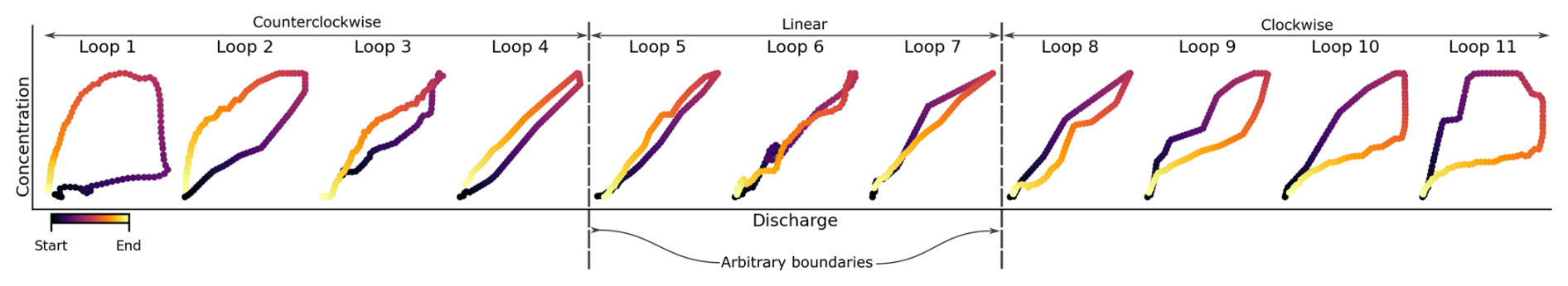
Figure 1 Examples of hysteresis loops arranged to show the smooth transition from wide counterclockwise loops (left), through linear loops (center), to wide clockwise loops (right). The figure demonstrates the limitations of traditional classification schemes which rely on rigid boundaries that fail to account for the gradual transition between loop types. For instance, if loops are classified based on the depicted boundaries, the similarity between loop 4 and loop 5 would not be captured. This classification scheme would, in fact, treat loop 4 and loop 5 as being as categorically distinct as loop 1 and loop 5, despite the clear similarities. The depicted hysteresis loops are derived from turbidity and discharge data collected by the USGS across eight different watersheds (see Sect. 3.1.1).

The use of hysteresis indices addresses some of these limitations. They can be automated for large datasets and preserve some of the continuous variability of hysteresis loops. For instance, the indices proposed by Zuecco et al. (2016) and Lloyd et al. (2016) – which are among the most commonly used – range from −1 to 1, reflecting the transition from counterclockwise to clockwise, with zero indicating the absence of a loop (single line). While these hysteresis indices has proven effective for revealing information about dominant hydrologic processes in watersheds (Liu et al., 2021; Zarnaghsh and Husic, 2021; Marin-Ramirez et al., 2024), they often fail to capture meaningful differences in loop shape. For example, the hysteresis index values (as calculated following Zuecco et al., 2016) of the clockwise loops in Fig. 2 are equal despite presenting significant qualitative differences, not just in the loop shape itself, but in the characteristics of the discharge and concentration pulses. Particularly, Event 1 and Event 2 differ in their concavity (concave-up and concave-down, respectively) which reflects differences in the relative spread of the discharge and concentration pulses (Williams, 1989). As shown in the lower panel of Fig. 2, concave-up loops occur when the concentration pulse is narrower than the discharge pulse, whereas concave-down loops indicate a wide concentration pulse, likely reflecting a persistent source that remains active during the receding limb of the event. Event 3 on the other hand, shows an extreme case of a leading concentration pulse, where the concentration rises and recedes almost entirely during the rising limb of the hydrograph producing an “L” shaped loop. This loop shape suggests a strong decoupling between stream discharge and concentration. Despite these differences, the hysteresis index of each loop in Fig. 2 is identical, demonstrating its limitation to capture loop features relevant for distinguishing transport mechanisms and/or sources.

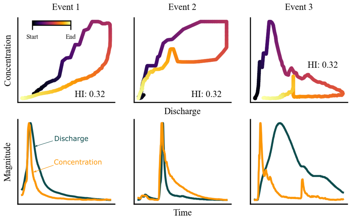
Figure 2 Examples of hydrologic events with hysteresis loops that yield identical hysteresis index values (as defined by Zuecco et al., 2016) despite notable differences in their C–Q relationships. For instance, the variation in concavity between events 1 and 2 reflects differences in the width of the concentration pulse, while the distinctive “L”-shaped loop in event 3 suggests a decoupling between stream discharge and concentration. These examples illustrate the limitations of hysteresis indices in capturing critical differences in loop shapes that are essential for characterizing transport dynamics. The depicted loops are based on turbidity and discharge data collected by the USGS from three watersheds (see Sect. 3.1.1).

To overcome the limitations of traditional classification schemes and hysteresis indices, we propose characterizing discharge-concentration hysteresis loops using Self-Organizing Maps (SOM). SOM is an unsupervised machine learning algorithm (Kohonen, 1990) widely used for clustering, dimensionality reduction, and data visualization. Although extensively used in water resources (Kalteh et al., 2008; Clark et al., 2020), to our knowledge, its potential for characterizing hysteresis loops has yet to be explored. When applied to C–Q hysteresis loops, SOM generates a two-dimensional map, also called a Kohonen map, that may enable improved representation of loop type variability, deeper exploration of loop characteristics, and enhanced interpretation of diverse C–Q relationships. Furthermore, the algorithm may support key workflows in hysteresis analysis, including data visualization, clustering of similar loop patterns, and correlation analysis to uncover potential controls on loop types, while taking advantage of machine learning's ability to analyze large datasets.

In this technical note, we evaluate the efficacy of the SOM algorithm to represent hysteresis loop patterns and discriminate hysteresis loop types, compared to traditional classification schemes and hysteresis indices. We use a dataset of turbidity (as a proxy for sediment concentration) and discharge to provide a proof-of-concept for using SOM to discriminate and characterize loop types commonly seen in sediment transport literature. In the following sections, we: (i) present a brief description of the SOM algorithm and explain its application for C–Q hysteresis analysis (Sect. 2), (ii) present a proof-of-concept for the use of SOM to analyze turbidity–discharge hysteresis loops (Sects. 3 and 4), (iii) compare results from SOM with the hysteresis index and discuss its efficacy in discriminating samples between different loop types (Sect. 4), and (iv) show how to use the SOM algorithm with data from any watershed (regardless of the number of hysteresis loop samples available) to describe the distribution of loop patterns and explore the association between loop types and their potential controlling factors (Sects. 4 and 5). Finally, to support broader adoption of the methodology described in this paper, we have developed a Python package – HySOM – equipped with detailed documentation to facilitate SOM implementation and application in future C–Q analysis (Code and data availability section).

2 Self-Organizing Maps for C–Q hysteresis analysis

2.1 Brief description of SOM

The SOM algorithm (Kohonen, 1982, 1990) is an unsupervised learning technique widely applied in various fields, including clustering, classification, manifold learning, dimensionality reduction, and data visualization (Miljković, 2017). In water resources, SOM has been applied for diverse purposes such as rainfall-runoff modelling, regionalization, clustering of water quality data, analysis of land use and land cover, and more (Kalteh et al., 2008; Clark et al., 2020). The algorithm generates a discrete representation of a dataset known as a feature map or Kohonen map (Miljković, 2017), which typically takes the form of a two-dimensional grid of nodes arranged in either a rectangular or hexagonal lattice. Each of these nodes represents a prototype of similar samples in the training dataset. The spatial arrangement of prototypes on the map preserves the topological structure of the input training data such that similar prototypes are placed close to each other, while dissimilar prototypes are placed farther apart. In the context of hysteresis, the input samples to the SOM algorithm are paired sequences of discharge and concentration data, each of them representing a hysteresis event, and the output of the SOM algorithm is a set of prototype loops that represent characteristic C–Q behavior arranged in a continuum. In the following subsections we will explain how SOM can be applied to hysteresis analysis. We have also included a glossary in the SI with key SOM terminology to facilitate understanding for readers who may be unfamiliar with the algorithm.

2.2 A two-phase workflow for applying SOM in hysteresis analysis

We propose using SOM for C–Q hysteresis analysis following the two-phase workflow illustrated in Fig. 3. The Training and evaluation phase involves constructing an SOM to represent the spectrum of hysteresis loop types associated with a specific dissolved or particulate constituent. To ensure the trained SOM adequately captures the diversity of loop patterns, we recommend curating a training dataset that includes a similar number of representative examples of all known loop types for the constituent under investigation. This curated dataset serves three key purposes: (i) to represent the known hysteresis loops for a given constituent, thereby ensuring broad applicability of the resulting SOM; (ii) to guarantee representation of less frequent patterns; and (iii) to provide a reference for evaluating the SOM's ability to distinguish loops in line with conceptual classifications (last step of the Training and evaluation phase, Fig. 3). More details on the training and evaluation procedures are provided in Sect. 2.3.

The output of the first phase is a trained SOM composed of coherently arranged prototypes reflecting the range of loop types in the training dataset. For instance, along with this technical note, we released a trained SOM for sediment transport hysteresis analysis – referred to as the General T–Q SOM – which is publicly available for use in sediment hysteresis analysis studies (Code and data availability section).

The Analysis phase consists of using the trained SOM to classify loop types in new datasets, provided they correspond to the same constituent of interest. First, each loop in the dataset is mapped to its most similar loop prototype. This classification enables systematic analysis of hysteresis patterns across watersheds. For example, by quantifying the number of samples assigned to each prototype, researchers can characterize the frequency distribution of loop types and investigate their associations with hydrological variables, thereby providing valuable insights into the underlying controlling mechanisms, as demonstrated in Sect. 4.

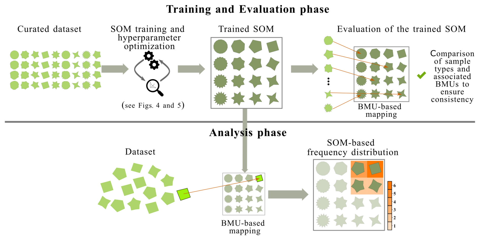
Figure 3 Workflow to generate an SOM for C–Q hysteresis loops (Training and evaluation phase) and apply the SOM for C–Q hysteresis analyses in watersheds (Analysis phase). Here, we illustrate the generation of the SOM using different shapes, which are analogous to the hysteresis loop types that might be found for a dissolved or particulate constituent in a watershed. In the bottom panel (Analysis phase), we demonstrate how hysteresis loops from a new dataset get mapped to the trained SOM, where the shade of orange represents the frequency with which the shape occurs in the dataset. The HySOM python package (see Code and data availability section) allows users to implement both phases of this workflow. BMU (Best-Matching Unit) refers to the prototype that best represents a given sample.

2.3 Training and evaluation phase

2.3.1 Input data: Representing hysteresis loops for SOM

In Fig. 3, samples (in light green) are depicted as geometric shapes for illustrative purposes. However, the SOM algorithm requires that input data be represented as numeric arrays. In conventional SOM applications, each sample is represented as an n-dimensional vector. Similarly, the resulting prototypes are vectors of the same dimension. For C–Q hysteresis analysis, we propose representing each loop as a sequence of paired discharge-concentration values, forming a matrix with dimensions n×2, where n indicates the number of data pairs used to represent the loop. n therefore may be equal to the number of entries in the C–Q time series, however because hydrologic events usually vary in duration, we recommend resampling the data such that hysteresis samples and prototypes each share a consistent dimension. We expand on this in Sect. 3.

Alternative formats for samples and prototypes are also possible. For instance, Hamshaw et al. (2018) encoded loops as greyscale images with a resolution of 28×28 pixels for use in a classification algorithm. However, in our implementation, representing loops as sequences of (Q, C) pairs yielded better results through the SOM algorithm.

2.3.2 SOM training

Training setup

As a preliminary step prior to training, several components of the SOM algorithm must be specified, including a distance function, a decay function, and a neighborhood function, which together control how input samples are compared and organized within the low-dimensional lattice during SOM training. We adopt standard formulations for the decay and neighborhood functions commonly used in SOM applications, as described in Sect. 2.3.2 “Training algorithm” and shown in Fig. 4. However, we provide greater explanation regarding our choice of distance function, as its application to hysteresis analyses warrants additional consideration.

The distance function is a critical element of the SOM algorithm as it measures the similarity between a sample and each prototype. In the context of hysteresis, the distance function measures the similarity (or dissimilarity) between two hysteresis loops. This function directly affects the SOM algorithm's ability to extract the main patterns from the input data and arrange them in a coherent manner. Furthermore, this function is required during the Analysis phase (Fig. 3) to map new hysteresis data to their associated loop prototype (BMU). While Euclidean distance is the default selection in most SOM applications, any function that computes the degree of similarity between two numeric arrays can be used such as Cosine similarity, Manhattan distance, Minkowski distance, etc. (Samarasinghe, 2016). Given our representation of hysteresis loops as sequences of Q–C data pairs, we propose using Dynamic Time Warping (DTW) to measure similarity between loops for application with SOM for hysteresis analysis.

DTW is an algorithm that measures the similarity between two timeseries that may have slight timing mismatches. It has proven effective in clustering and classification across various domains involving sequential data (Ding et al., 2008; Dupas et al., 2015; Shokoohi-Yekta et al., 2017; Lee et al., 2020). Its primary advantage lies in its ability to prioritize the overall shape of the temporal sequences over a strict match of individual data points comprising the sequence. This is achieved by non-linearly stretching or compressing the time axis of one sequence to achieve optimal alignment with another, prior to computing the Euclidean distance between the aligned sequences. The resulting DTW distance reflects this alignment: it is upper bounded by the Euclidean distance when no alignment is possible, but yields a lower value when warping improves the match, indicating greater shape similarity. A comparison between Euclidean and DTW distances is presented in the Supplement (Sect. S2).

Training algorithm

The SOM training algorithm for hysteresis analysis is illustrated in Fig. 4. First, training hyperparameters must be set. This includes the number of nodes in the map lattice, which thereby determines the number of prototypes (and, therefore, the number of distinct loop types) to be included in the trained map. While a larger map can represent a dataset with higher accuracy, they are often more difficult to visualize and interpret. Additionally, larger maps may produce prototypes that represent too few or none of the input samples, making the results more susceptible to noise and outliers. Ultimately, defining the map size relies on heuristic rules, domain intuition, and visual examination of the dataset (Vesanto, 2000; Kohonen, 2013). Importantly, however, the optimal size of the map should be refined iteratively (see Sect. 2.3.3 and Fig. 5), expanding the number of nodes until increases no longer result in meaningful improvements in the quality of the map (Céréghino and Park, 2009). We discuss metrics to assess the map quality in Sect. 2.3.3.

Additional hyperparameters include the initial and final learning rate (α₀, α_f) and neighborhood radius (σ₀, σ_f). As explained below, they control the degree to which the map prototypes are adjusted during each step of the training process. The final hyperparameter is the number of epochs (an epoch is a training iteration where the entire dataset is processed once), which controls the length of the training process.

Once the map size is defined, initial prototypes must be assigned to each node. Random initialization using samples from the training dataset is commonly used, although more elaborate initialization approaches can also be employed (Attik et al., 2005). In the context of hysteresis, this means that a random set of hysteresis loops from the training dataset would be used to initialize the prototypes, which are then refined throughout the training process.

With this initial, untrained map, the training process is conducted by sequentially feeding random samples and adjusting the prototypes to better match the input data (see Training loop in Fig. 4). For each sample X, the BMU is identified as the node whose prototype exhibits the highest similarity to the input sample as measured by the DTW function. Once the BMU is identified, the learning parameters for the current iteration – learning rate (α) and neighborhood radius (σ) – are computed using a decay function. This decay function gradually reduces α and σ, resulting in a transition during training from an initial ordering and placement phase where prototypes broadly align with the spatial structure of the input data, to a fine-tuning phase where prototypes are refined to better represent the input samples (Samarasinghe, 2016).

Common choices of decay functions include hyperbolic, exponential, and linear (Kohonen, 2013). In our implementation, we adopted an exponential decay rate which varies from initial to final values defined during the map initialization (see Compute learning parameters in Fig. 4). In the next step of the training loop, neighborhood values $\left(h_{\mathrm{BMU},{\mathit{\eta }}_k}\right)$ are computed. These values control the extent to which the prototype of each node η_k is updated during the current iteration based on the Euclidean distance – in map coordinates – between η_k and the BMU. This function plays a critical role in enabling SOM to produce smooth transitions across neighboring prototypes (i.e., ensuring that similar hysteresis loops are placed near one another). The neighborhood value reaches its maximum at the BMU and decreases with increasing distance from it, with the rate of decay being controlled by σ. In our implementation, we used the Gaussian kernel (see Compute neighborhood function values in Fig. 4), which is the most commonly used neighborhood function in SOM applications (Kalteh et al., 2008).

Finally, the prototype ${\mathbf{m}}^{{\mathit{\eta }}_k}$ of each node η_k is updated using the learning rule (see Update prototypes in Fig. 4), which adjusts the prototypes toward the input sample. In the context of hysteresis, each prototype loop is iteratively refined to resemble C–Q hysteresis loops in the training data. This learning rule ensures that both the BMU and its neighboring nodes are moved closer to the current sample, allowing nearby prototypes to become more similar, which preserves the continuity of patterns across the map. The magnitude of adjustment decreases over time and with distance from the BMU, as determined by the decay and neighborhood functions.

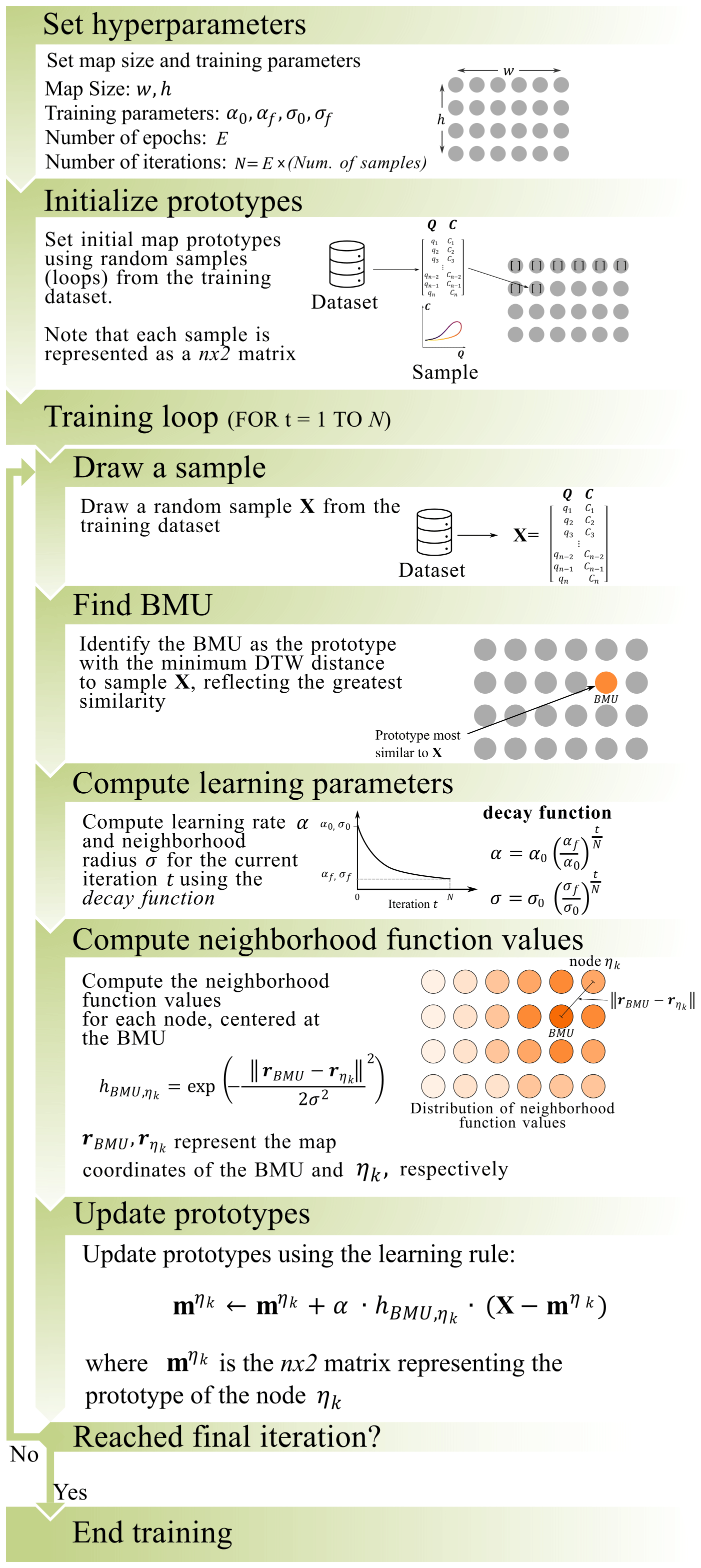
Figure 4 Workflow for training an SOM. α: learning rate, σ: neighborhood radius, subscripts , f indicate initial (first iteration) and final (last iteration) values, respectively. Q: Discharge, C: Concentration, n: length of the sequence of (QC) data pairs representing a loop (Sect. 2.3.1). Other symbols are defined in the figure.

2.3.3 Hyperparameter optimization

Training hyperparameters – such as map size, learning rate, and neighborhood radius – directly influences the SOM's ability to preserve data topology and accurately represent input samples. To guide hyperparameter selection, we rely on two widely used SOM quality metrics: topographic error and quantization error. These metrics provide complementary insights into the structural fidelity and representational accuracy of the trained map.

Topographic error quantifies the degree to which the SOM preserves the topological structure of the input space, that is, how well it maintains neighborhood relationships between loop types. A low topographic error indicates that similar loop prototypes are positioned close together, while dissimilar ones are placed farther apart. In the context of hysteresis, this means that loops with similar amplitude, rotational direction and shape should be placed close together. This metric is defined as the fraction of samples for which the Best Matching Unit (BMU) and the second BMU (i.e., the prototype with the second smallest distance to the input vector) are not adjacent on the map (Kiviluoto, 1996; Pölzlbauer, 2004). Lower values are preferred.

Quantization error, on the other hand, measures how closely hysteresis prototypes approximate the input hysteresis samples. It is defined here as the average DTW distance between each sample and its BMU (Pölzlbauer, 2004). Lower quantization errors indicate improved accuracy.

These two metrics often represent competing objectives as reducing one metric may increase the other. Therefore, a balance must be achieved by evaluating SOMs trained under varying hyperparameter configurations. These configurations should simultaneously consider:

• Map size. Increasing the number of nodes generally reduces quantization error, as more prototypes can better approximate the dataset. However, larger maps may complicate visualization and interpretation. In the context of hysteresis analysis, the map size determines the number of distinct loop types to be included in the trained map.

• Neighborhood radius. A wider radius promotes smoother transitions between hysteresis prototypes, reducing topographic error but potentially increasing quantization error. Conversely, a narrower radius sharpens prototype specialization, improving quantization error such that hysteresis loops are mapped to their prototypes relatively well, but risking topological fragmentation, which can result in dissimilar hysteresis loops being placed close together.

• Learning rate. This influences the speed and stability of convergence, with its decay profile affecting both error metrics.

In addition to quantitative metrics such as topographic and quantization errors, SOMs trained on hysteresis loops can be evaluated qualitatively as the prototype distribution can be easily visualized. The spatial distribution of prototypes offers a visual indication of topological preservation, with smooth and coherent transitions between loop types serving as a desirable trait.

To fine-tune training hyperparameters, we propose the workflow illustrated in Fig. 5. First, multiple SOMs are trained across a grid of map sizes, learning rates, and neighborhood radii. The optimal map size is identified by examining the relationship between quantization error and number of nodes. While a decreasing trend in quantization error is expected as the number of nodes increases, the elbow method (Nainggolan et al., 2019) helps pinpoint the optimal number of nodes for a map. Once the optimal size is selected, a subset of high-quality maps – trained with varying learning rates and neighborhood spreads – is extracted for closer inspection. These maps are chosen from the Pareto frontier (Koppa et al., 2019) of topographic and quantization errors.

Visual assessment of these maps is then performed, guided by conceptual understanding of loop type similarities. In this application, we prioritized maps that exhibited smooth transitions between similar loop types and clear separations between contrasting ones. Finally, we recommend further retraining the selected SOM to further improve map quality. While the initial selection from the Pareto frontier emphasized topological arrangement, retraining enhances quantization accuracy, yielding final error metrics that surpass the original Pareto frontier.

Figure 5 Workflow for fine-tuning SOM hyperparameters using a combination of quantitative metrics and qualitative assessment. The process begins with training multiple SOMs across a grid of map sizes, learning rates, and neighborhood radii. Quantization error is evaluated to identify the optimal map size using the elbow method. A subset of high-quality maps – selected from the Pareto frontier of topographic and quantization errors – is then examined in detail. SOM selection is based on visual inspection, prioritizing maps that exhibit coherent transitions between similar loop types and clear separation between contrasting ones. Finally, retraining of the selected SOM may enhance quantization accuracy.

2.3.4 Evaluation of a trained SOM

The final step of the training and evaluation phase (see Fig. 3) involves assessing the SOM's ability to represent the full spectrum of loop types included in the curated dataset. We propose visual inspection as the most suitable approach, as it allows researchers to assess whether the distribution of prototypes reflects the diversity of loop shapes in the curated dataset and whether their arrangement aligns with conceptual expectations of loop similarities and differences. For instance, in our proof of concept, we examined whether loops from closely related classes (e.g., async-peak and sync-peak; see Fig. 6) were mapped to neighboring prototypes – indicating the SOM's ability to recognize shared geometric traits.

This evaluation helps identify which loop features are effectively captured by the SOM and which may require more nuanced analysis. Crucially, because SOM training is fully unsupervised, it does not rely on manual labels; instead, it organizes loops based solely on shape similarity, as defined by the DTW distance function.

Although quantitative metrics such as confusion matrices could be used to assess classification performance, we recommend not to apply them here. Such metrics would require converting the SOM output into discrete categories, undermining its key advantage: preserving smooth transitions and continuous variation between loop types.

2.4 Analysis phase

Once the SOM has been trained, it can be used to classify hysteresis loops in new datasets. For each new loop, the two-dimensional Q–C sequence is compared against all map prototypes using the same distance function employed during training (i.e., DTW). The prototype yielding the minimum distance is identified as the BMU, and the loop is assigned to the corresponding map node. Applying this procedure to all samples in a dataset enables the results to be visualized as heatmaps, as illustrated in Fig. 3. In addition to visualizing the frequency of loop-type assignments, associations between loop types and hydrologic variables can be explored by mapping the corresponding variable values onto the SOM lattice. This approach is demonstrated in detail in the proof-of-concept presented below.

3 Applying SOM to turbidity-discharge hysteresis loops

We employ turbidity–discharge (T–Q) data to develop a proof-of-concept and demonstrate the proposed workflow for training and applying SOM for C–Q hysteresis analysis described in Sect. 2 and Fig. 3. The output of the training and evaluation phase for the proof-of-concept is what we refer to as the General T–Q SOM. We stress, however, that this workflow is adaptable to other constituents such as nutrients, dissolved solids, metals, and more. Future studies are encouraged to explore its application across a broader range of constituents.

3.1 Training and evaluation phase

3.1.1 Data curation and preprocessing

We surveyed the sediment transport literature to compile the primary loop types included in the curated dataset (Fig. 6). Our review indicates that the majority of sediment hysteresis loop types recognized in the literature were originally identified by Williams (1989), with the Figure L loop introduced by Hamshaw et al. (2018). Additional studies have introduced nuanced variations of these loop types; for example, Bettel et al. (2025) introduced the “J” loop for a karstic system in Kentucky, USA which resembles concave-up loops. However, our analysis suggests that sediment hysteresis loop diversity can largely be explained by the 17 loop types identified in Fig. 6, encompassing single-line (first row in Fig. 6), clockwise (second row in Fig. 6), and counterclockwise (third row in Fig. 6) topologies. Irregular loops (e.g., complex loops) were excluded due to their abnormality and lack of a standardized classification system. While additional loop types may exist beyond those included, they are generally infrequent and relevant only to specific studies or watersheds. Therefore, since our training dataset incorporates most of the known sediment hysteresis loop types, we refer to the output of the training and evaluation phase as the General T–Q SOM. We discuss the incorporation of less common loops in Sect. 5 and encourage the development of tailored SOMs to accommodate specialized applications.

The curated dataset consists of 20 samples for each loop type, resulting in a total of 340 loops. These loops come from hydrologic events which were manually delineated from publicly available discharge and turbidity data collected by the USGS at 15 min intervals across 37 stream gauges in the United States. Data were retrieved from the National Water Information System using the Data Retrieval Python package (Hodson et al., 2023). Event delineation was supported by a custom-built application designed to manually label hydrologic time series.

Watershed selection and event delineation followed the criteria outlined below:

• Only rainfall-dominated hydrologic events were included; heavily regulated rivers and snowmelt-dominated watersheds were excluded.

• Multi-peak events were split into single-peak events if turbidity receded fully before the onset of the subsequent peak.

• Irregular loops (such as complex loops) or loop shapes that did not conform to the typologies illustrated in Fig. 6 were excluded.

• We then manually classified the loop shape to one of the typologies illustrated in Fig. 6 according to visual comparison until an even number of event types was identified.

We should note that while manual classification during data curation can be somewhat subjective, this is a minor concern since the SOM is not constrained to enforce strict boundaries between loop types and does not see the assigned labels. For example, whether a narrow clockwise loop is labeled as a single line or a clockwise Sync-Peak loop may be debatable – but including it in training allows the SOM to learn the gradual transition between these shapes, independent of the assigned label. Additionally, while dataset curation is a time-intensive task, requiring the extraction of multiple hydrologic events from several watersheds, it is typically performed only once for each constituent. Once trained, the SOM can be readily shared and reused by other researchers without the need for retraining.

The Supplement provides detailed site information and data periods (Table S1), while the complete set of loops included in the training dataset is presented in Fig. S3.

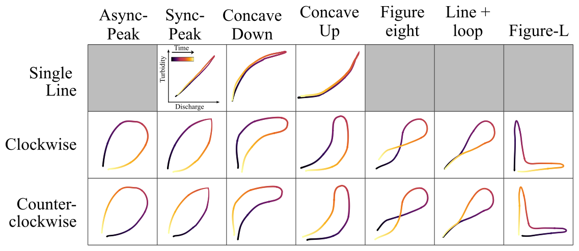
Figure 6 Loop types considered in the training dataset. Except for Figure-L loops – introduced by Hamshaw et al. (2018) – all loop types were originally described by Williams (1989). While past studies often lump together all subclasses within the broader categories of Single Line, Clockwise, and Counterclockwise loops, our dataset introduces a more granular classification that captures multiple shape variations within each type, such as differences in concavity, which reflect the relative spread of the sedigraph with respect to the hydrograph, or Figure-L loops, which indicate strong decoupling between discharge and sediment concentration. Readers interested in the hydrological interpretation of these loop types are encouraged to consult the original studies.

The SOM algorithm requires samples to be represented as arrays with an equal number of elements. Given that loops in the dataset consist of variable-length sequences of Q–T data pairs, we implemented a preprocessing procedure to convert all loops into sequences of equal length, ensuring compatibility with the SOM algorithm. This procedure is illustrated in Fig. 7 and involves the following steps. First, we applied a moving median with a 5-point window to the turbidity values to reduce random noise (Fig. 7b). Second, the Q–T data were scaled to a [0,1] interval using min–max normalization based on the minimum and maximum values for each event. This scaling, commonly applied prior to the calculation of hysteresis indices, facilitates comparison between loops of different magnitudes (Lloyd et al., 2016); and third, we interpolated the resulting variable-length, scaled T–Q data (Fig. 7c) to produce equal-length sequences (Fig. 7d) of 100 data pairs. The interpolation ensures that data points are equally spaced in the Q–T plane.

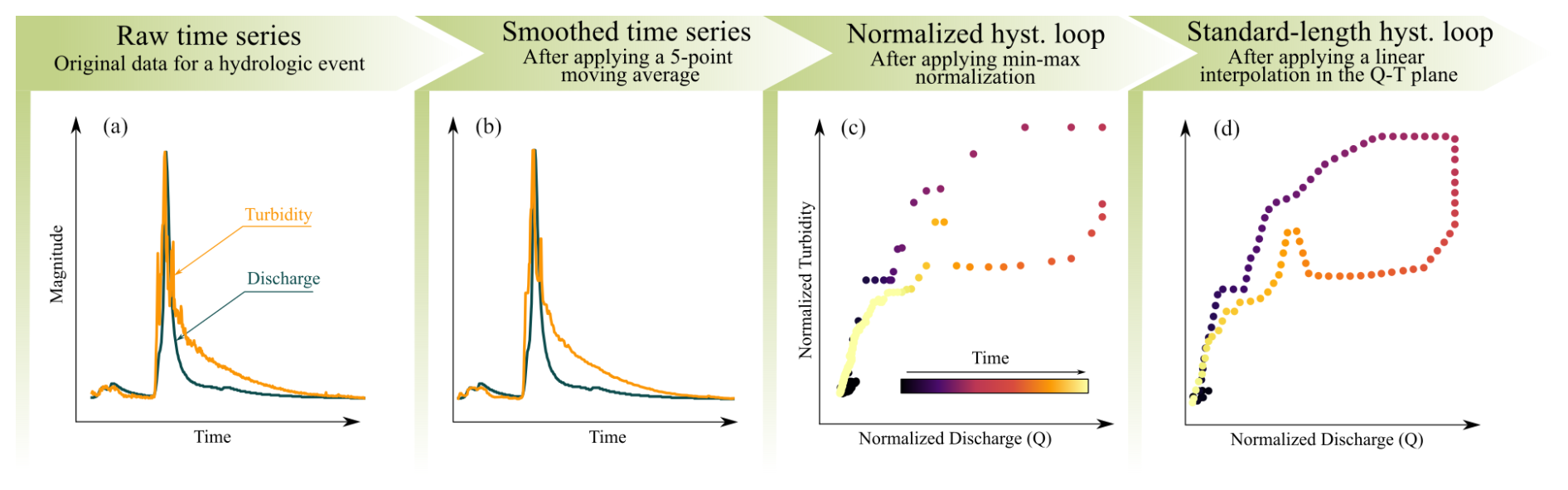
Figure 7 Workflow illustrating data preprocessing steps: (a) original discharge and turbidity data, (b) a 5-point moving median was applied to turbidity data to mitigate outliers, (c) Q–T data were min-max normalized to a [0,1] interval, (d) the scaled, variable-length data were interpolated into equal-length sequences of 100 data pairs.

3.1.2 SOM training and hyperparameter optimization

SOM training and hyperparameter tuning followed the workflows explained in Sect. 2.3. SOM sizes ranged from 5×5 to 13×13 nodes, with initial neighborhood radii varying from 0.5 to 13 and initial learning rates from 0.05 to 0.9. Final values for neighborhood radius and learning rate were set at 0.3 and 0.01, respectively. Training was conducted over five epochs, meaning the entire dataset was presented to the algorithm five times, resulting in 1700 iterations per hyperparameter combination (340 samples × 5 epochs). In total, approximately 900 SOMs were trained.

The training algorithm was implemented in Python, using the Numpy library (Harris et al., 2020) for array computations and the DTW implementation provided by the tslearn package (Tavenard et al., 2020). Training time per SOM ranged from 20 s for smaller maps (5×5 nodes) to 140 s for larger maps (13×13 nodes), with a total execution time of approximately 15 h on an AMD Ryzen 9 PRO 5945 12-Core Processor (3.00 GHz). It is important to note that this computing time applies only to the training phase. Once trained, the SOM can classify hundreds of loops in a fraction of a second using the DTW algorithm.

Optimal SOM selection, as illustrated in the fourth step of Fig. 5, was guided by our conceptual understanding of sediment transport loop types. For instance, maps were prioritized when clockwise and counterclockwise Figure L loops were placed farther apart than clockwise and counterclockwise Sync-Peak loops (see Fig. 6), reflecting the greater temporal mismatch between discharge and turbidity in the former. This conceptual prioritization helped ensure that the SOM captured meaningful distinctions in loop behavior.

In the final refinement step, the selected SOM was retrained for an additional five epochs to enhance quantization accuracy. While the initial training emphasized the overall arrangement of loop types, this refinement focused on improving the alignment between each BMU and its associated samples. To achieve this, a constant neighborhood spread of 0.45 and learning rate of 0.05 were employed.

3.1.3 Evaluation

We followed the principles defined in Sect. 2.3.4 to evaluate the trained SOM's ability to represent the full spectrum of loop types in the curated dataset. Specifically, we visually examined whether loops from the same or similar categories (e.g., single-lines) were consistently mapped to prototypes that reflect their characteristic shapes. We also assessed the extent to which the SOM distinguished between conceptually contrasting C–Q dynamics, such as clockwise versus counterclockwise Figure L loops, indicating its capacity to capture meaningful differences in loop behavior.

3.2 Analysis phase

We demonstrate the application of the trained and evaluated T–Q SOM (referred to henceforth as the General T–Q SOM) for analyzing hysteresis patterns using a secondary dataset, not used during training, consisting of T–Q hysteresis loops from three monitoring stations. These watersheds were selected to illustrate two primary analyses for characterizing hysteresis patterns: (1) exploring the frequency distribution of loop types within a watershed (gages 07364130 and 03254480), and (2) identifying associations between loop types and hydrologic variables (gage 03289000).

The coordinates of these stations and key properties of their associated watersheds are provided in Table 1. Watershed boundaries were obtained from the USGS StreamStats online application, watershed slope was calculated using the USGS 3DEP (10 m) digital elevation model, urban area was extracted from the 2021 National Land Cover Database, and soil texture was extracted from the Probabilistic Remapping of SSURGO (POLARIS) database (Chaney et al., 2019).

Table 1 USGS monitoring stations and watershed properties used in the SOM-based analysis phase.

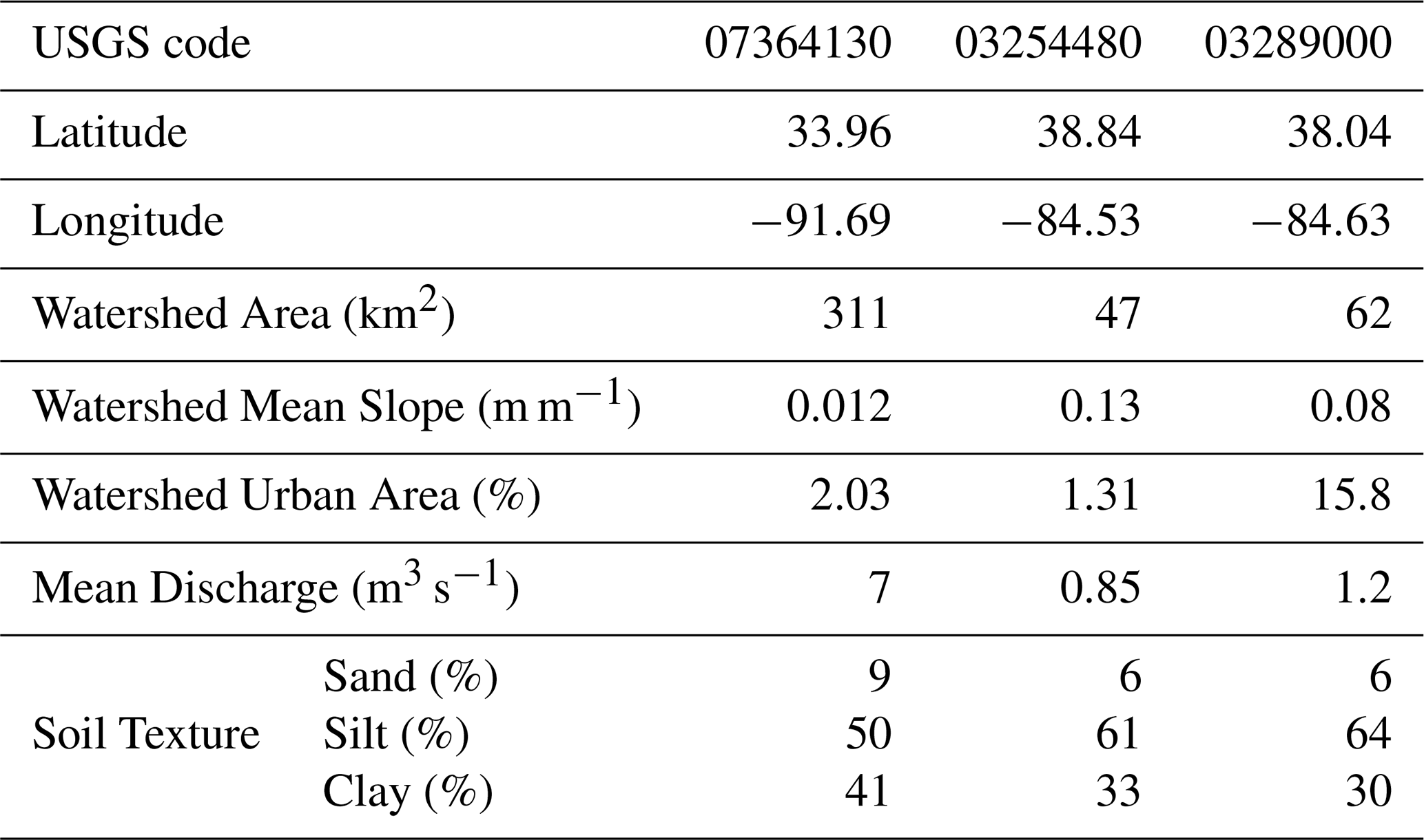
Hydrologic events for watersheds 07364130, 03254480, and 03289000 were manually extracted from 15 min discharge and turbidity data provided by the USGS and retrieved via the National Water Information System. For station 03289000, turbidity data were collected by the University of Kentucky using a YSI 6-series optical turbidity sensor. All loops underwent preprocessing consistent with the curated dataset (see Sect. 3.1.1). This process resulted in 27, 54, and 70 events for gages 07364130, 03254480, and 03289000, respectively. Additional hydrologic variables were included for watershed 03289000, including rainfall 15 h prior to events, average discharge over the 5 preceding days, and the ratio of old-water to event-water, derived from our previous work in this watershed (Marin-Ramirez et al., 2024). These variables serve as proxies for rainfall, antecedent moisture conditions, and dominant hydrologic pathways associated with each event, respectively.

For each site, loop frequency distributions were generated by mapping individual hysteresis loops to their corresponding BMU prototype and visualizing the results as heatmaps atop the General T–Q SOM. For gages 07364130 and 03254480, we compared these heatmaps to frequency distributions of hysteresis index, as proposed by Zuecco et al. (2016).

For watershed 03289000, the General T–Q SOM was employed to explore relationships between loop types and hydrologic variables. This watershed was selected based on prior understanding of the hydrologic processes controlling sediment transport in the watershed (Marin-Ramirez et al., 2024), providing a framework for validation and comparison with the trained General T–Q SOM. Associations between hydrologic variables and loop types were qualitatively explored through visual analysis, where median values of the variables were plotted across SOM prototypes as heatmaps to reveal patterns linking high or low values with specific loop types.

To further quantify these associations, we applied a correlation-based approach using multiple linear regression. The BMU coordinates of each loop served as predictor variables and the response variable was a rank-normalized hydrologic metric (precipitation, antecedent discharge, and the ratio of old-water to event-water). Rank-normalization enabled the model to capture non-linear, monotonic relationships. However, non-normalized variables could also be employed. Correlation coefficients quantified the strength of associations, while the regression-plane coefficients indicated the direction of maximum change in the hydrologic variable across the General T–Q SOM. These gradients helped identify which loop types were associated with higher or lower values of the hydrologic variables. Results were visualized using a biplot chart, enabling simultaneous exploration of relationships between loop types and multiple hydrologic variables.

4 Results

4.1 Training the General T–Q SOM

4.1.1 Balancing quantization and topographic errors

The elbow method identified 8×8 nodes as the optimal map size for the General T–Q SOM, where quantization error stabilizes (Fig. 8a). While larger maps may achieve lower quantization errors, this improvement comes at the cost of increased distortion, reflected by high topographic errors. Moreover, visual inspection of maps with varying sizes (not shown) revealed no advantages in terms of the number of loop patterns represented.

The pareto frontier of these 8×8 maps shows the expected inverse relationship between topographic and quantization errors (Fig. 8b). After visually examining six maps along this frontier, the map with the best overall distribution of loop types was selected (black dot shown in Fig. 8b). We favored maps with clear separations and smooth transitions between clockwise and counterclockwise loops and between concave-up and concave-down loops, which are representative of both the timing and duration of sediment transport during events (refer to Sect. S4 in the Supplement for an example of a discarded SOM). The selected map exhibited a low topographic error (0.006) but a relatively high quantization error (0.73). However, the quantization error was improved during the refinement phase. The final map achieves a well-balanced trade-off between topological preservation (TE = 0.04) and quantization error (QE = 0.66).

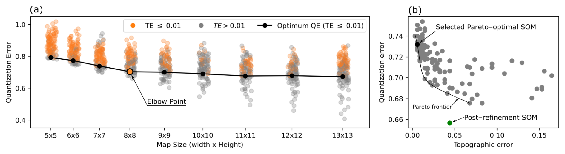
Figure 8 (a) Quantization Error (QE) across varying map sizes, illustrating the expected decrease in QE as map size increases. While larger maps continue to lower the minimum QE, this reduction stabilizes when considering maps with low Topographic Error (TE ≤0.01). Similar stabilization patterns are observed across other TE thresholds (0.05 and 0.1). (b) Scatterplot displaying QE and TE for 8×8 maps. The map selected after visual inspection is highlighted, alongside the final QE and TE following map refinement training, which corresponds to the General T–Q SOM.

4.1.2 The General T–Q SOM: A trained SOM for sediment hysteresis analysis

Figure 9 shows the trained SOM generated using the curated T–Q dataset, which we refer to as the General T–Q SOM. The map provides an organized representation of most loop types from the curated dataset, with smooth transitions between different classes. In general, the map arranges loop shapes based on the loop amplitude, rotational direction (clockwise or counterclockwise), and concavity following the directions defined by the diagonals. These diagonals can be conceptualized as axes of a Cartesian plane: the diagonal running from the lower left to the upper right (LL-UR) represents variations in loop amplitude and rotational direction, while the diagonal from the upper left to the lower right (UL-LR) represents changes in concavity.

The LL-UR diagonal illustrates the expected progression between clockwise and counterclockwise loops as illustrated in Fig. 1. Wide clockwise and counterclockwise loops occupy the extreme ends of this diagonal, while single lines are positioned near the center of the transition. Figure L loops notably appear at opposite ends of this transition, emphasizing their role as extreme cases of clockwise and counterclockwise loops, as they represent a pronounced mismatch in concentration between the rising and falling limbs (Fig. 2). The UL-LR diagonal, on the other hand, captures the transition from concave-up to concave-down loops. Hence, all concave-up (clockwise, counterclockwise and single lines) loops are placed in the upper-left quadrant of the map, while concave-down (clockwise, counterclockwise and single lines) occupy the lower-right quadrant.

Furthermore, these diagonals effectively serve as symmetrical axes, highlighting the map's coherent and robust topological structure. For example, clockwise loops along the LL-UR diagonal (e.g., H1, G2, F3, E4) are mirrored by their counterclockwise equivalents (e.g., D5, C6, B7, A8).

Interestingly, the map also reveals the presence of loop types not explicitly considered during data curation. For instance, it distinguishes between concave-up and concave-down clockwise line+loop loops (e.g., prototypes C1 and H6), underscoring its ability to capture differences in concavity. On the other hand, Figure-eight loops are less accurately represented – they appear as narrow loops placed close to single lines (e.g., D4, E5). This suggests that the map may have less discriminatory power for Figure-eight loops.

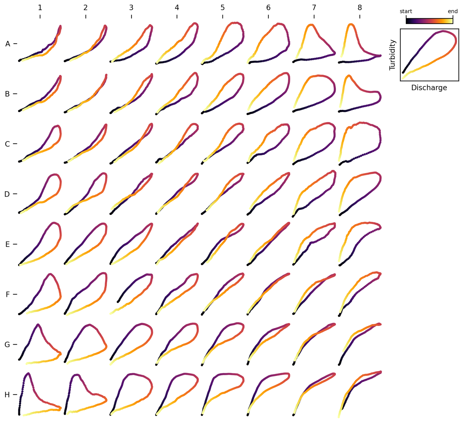
Figure 9 SOM for Turbidity–Discharge (T–Q) hysteresis analysis. The map was trained using a curated dataset comprising 17 different loop types, with 20 samples for each loop type. We refer to this as the General T–Q SOM.

4.1.3 Evaluation of the General T–Q SOM

To evaluate the efficacy of the trained SOM in discriminating between different loop types, we mapped each loop in our curated dataset to its corresponding prototype (i.e., its BMU). As shown in Fig. 10, the results are consistent with our manual classifications, noting that the manual classification was not seen by the model as part of the training process. In particular, the map effectively distinguishes rotational direction (clockwise, counterclockwise), loop amplitude (ranging from wide loops to single lines), and concavity. However, the self-intersecting structure of Figure-eight loops is less effectively captured.

Single-line loops are consistently mapped to prototypes that best represent their shape along the UL-LR diagonal (Fig. 10a), while Figure L loops are properly mapped to their corresponding prototypes at the map's corners (Fig. 10b, c). The spectrum of clockwise and counterclockwise loops (including Async-Peak, Sync-Peak, concave-down, concave-up and line + loop loops) is also well-represented, with clockwise loops occupying the lower-left quadrant and counterclockwise loops in the upper-left quadrant of the map (Fig. 10b, c).

Overlap exists between some loop types, which is expected due to the similar topologies of many loops (see Fig. 1). For instance, several counterclockwise Async-Peak and Sync-Peak loops map to the same prototype (prototype B6, Fig. 10c), while their clockwise counterparts group under prototype E2 (Fig. 10b). A closer examination of these clusters (Fig. 11) reveals that they comprise of loops sharing similar characteristics in terms of direction, amplitude, and concavity – or the lack thereof – demonstrating the algorithm's effectiveness in discriminating loops based on these features.

Figure-eight loops, in contrast, exhibit a more dispersed mapping, often associated with prototypes that lack a clear Figure-eight resemblance. Nonetheless, the mapping is not entirely flawed. Closer examination reveals that Figure-eight loops are matched to prototypes resembling their loop amplitude, direction, and concavity (see Fig. 11). Note that in our manual classification, these Figure-eight loops were categorized as clockwise based on the rotational direction of the second loop (i.e., the one with larger T–Q values). Nevertheless, they were mapped to counterclockwise loops following the rotational direction of the dominant loop, which in this case is the first loop. Despite this apparent contradiction, we consider this an acceptable representation of these loops.

Overall, we consider the trained SOM to perform satisfactorily when representing and discriminating between a broad spectrum of loop patterns associated with sediment transport, as informed by our survey of the sediment transport literature, therefore giving us confidence when referring to this trained SOM as the General T–Q SOM. Next, we explore specific uses of the General T–Q SOM for broader hysteresis analysis.

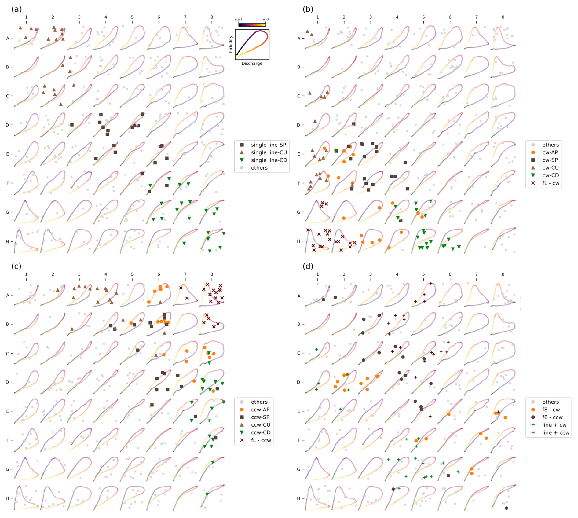
Figure 10 Mapping of all samples from the curated loop dataset to their respective BMUs on the trained SOM. For visual clarity, loop types and their mappings are organized into four distinct panels: (a) single-line loops; (b) clockwise loops including Async, Sync, Concave, and Figure-L; (c) counterclockwise loops including Async, Sync, Concave, and Figure-L; and (d) Figure-eight and Line+loops. Acronyms used in the figure include: SP: Sync-Peak, AP: Async-Peak, CU: Concave-Up, CD: Concave-Down, ccw: Counterclockwise, cw: Clockwise, fL: Figure-L, f8: Figure-eight.

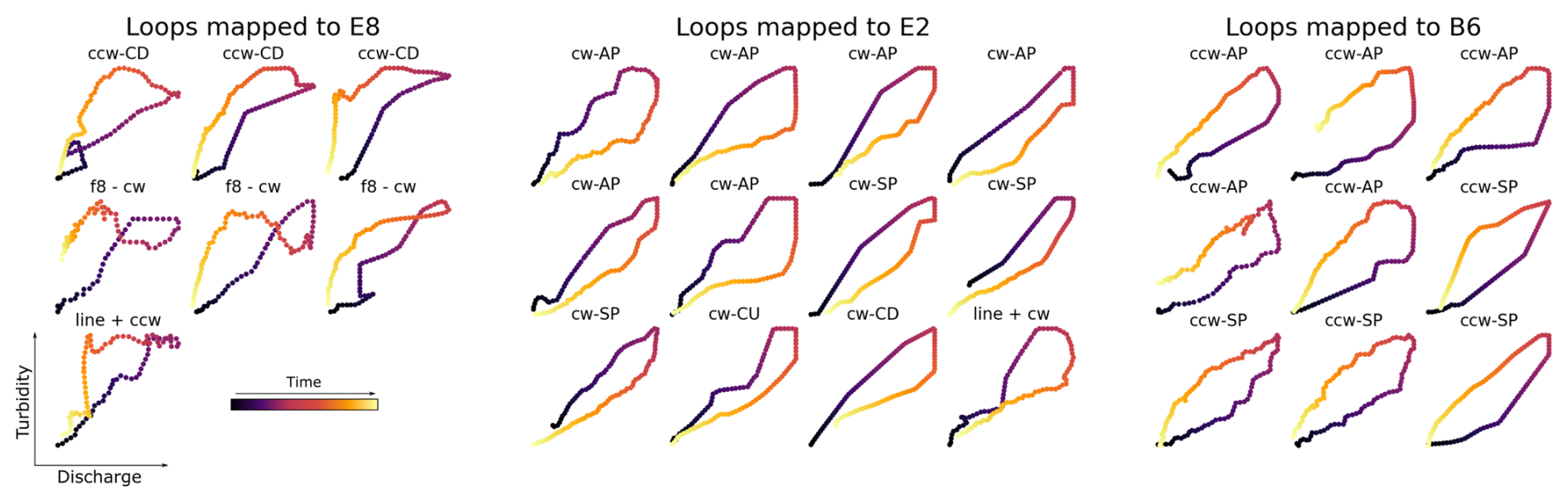
Figure 11 Loops mapped to prototypes E8, E2 and B6 along with their respective classes as defined in the manual classification. While loops from different classes in the curated dataset are mapped to the same prototype, this figure underscores their similarities in terms of loop direction, amplitude, and concavity – or the lack thereof. This highlights the inherently fuzzy boundaries that exist between certain loop types. SP: Sync-Peak, AP: Async-Peak, CU: Concave-Up, CD: Concave-Down, ccw: Counterclockwise, cw: Clockwise, fL: Figure-L, f8: Figure-eight.

4.2 Analysis of hysteresis loops using the General T–Q SOM

4.2.1 Characterizing frequency distributions of hysteresis loop types

Figure 12a shows the frequency distributions of hysteresis loop types found in watersheds 03254480 and 07364130 as heatmaps over the General T–Q SOM, contrasted with Fig. 12c, which shows the distributions of hysteresis index. While both watersheds predominantly exhibit clockwise loops, the General T–Q SOM reveals additional insights that the hysteresis index distribution cannot capture. Specifically, watershed 03254480 shows more concave-down loops, while watershed 07364130 primarily shows concave-up loops. These differences are overlooked by the hysteresis index, as its frequency distributions are statistically indistinguishable (two-sided Smirnov-Kolmogorov test, p=0.997).

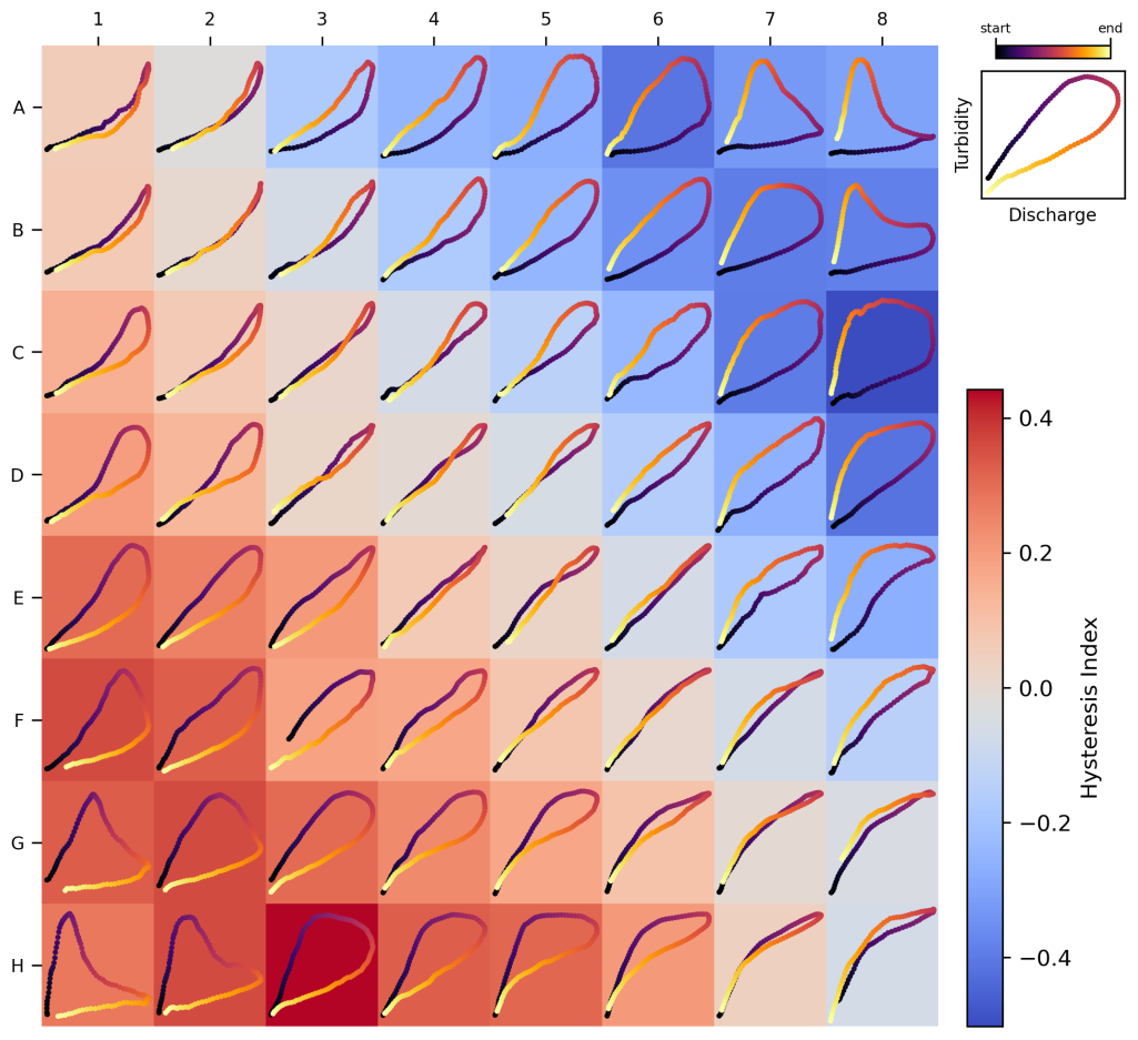
Figure 13 reinforces this by illustrating the distribution of hysteresis index values across the map's prototypes, confirming that the hysteresis index does not account for loop concavity. For instance, prototypes along the diagonal from E1 to H4 exhibit identical hysteresis index values, despite a noticeable transition from concave-up to concave-down loops. This highlights the General T–Q SOM's ability to capture subtle variations in loop characteristics that the hysteresis index fails to detect.

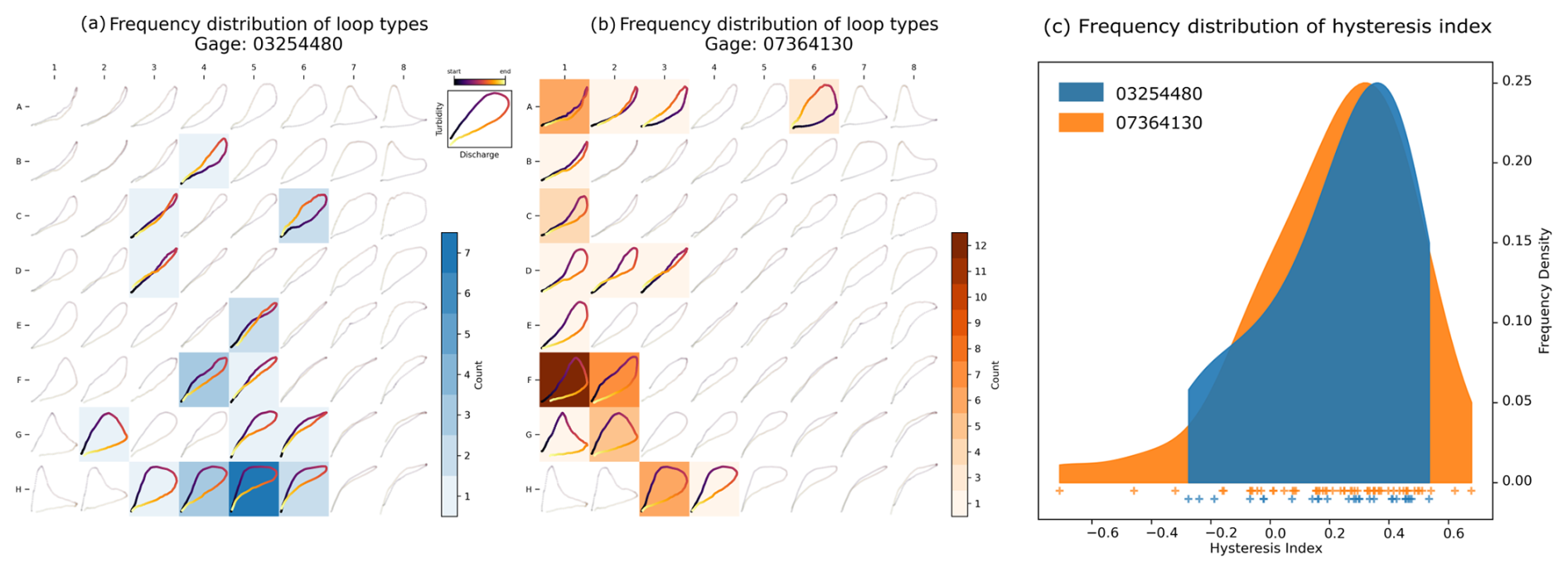
Figure 12 Frequency distribution of loop types for watersheds 03254480 (a) and 07364130 (b) mapped onto the General T–Q SOM and the hysteresis index (c). The frequency distributions mapped onto the General T–Q SOM reveal distinctions in loop types that are not captured by the hysteresis index.

Figure 13 Distribution of hysteresis index values across the General T–Q SOM.

Although a detailed analysis of the factors driving differences in loop types between watersheds 03254480 and 07364130 is beyond the scope of this technical note, the variations in frequency distribution displayed in Fig. 12a and b likely reflect differences in sediment transport mechanisms. Concave-down loops are typically associated with significantly higher sediment concentrations during the falling limb of the hydrograph compared to concave-up loops (See Fig. 2; Williams, 1989). This could be the result of differences in the watersheds's physiographic attributes. Gage 03254480, located in northern Kentucky at the outlet of a 47 km² watershed, is situated in hilly terrain with few flat areas (McGrain and Currens, 1978). In contrast, Gage 07364130, located in Arkansas at the outlet of a 311 km² watershed, is characterized by low-relief topography dissected by meandering rivers and streams, typical of the alluvial plain of the Arkansas and Mississippi Rivers. The hydrologic regime of 07364130 is likely more base-flow dominated than that of 03254480, a condition that has been linked to the formation of concave-up loops in previous research (Bettel et al., 2025). While this explanation remains speculative and requires further analysis for validation, the General T–Q SOM proves valuable in identifying variations in hysteresis loops that might have been overlooked with traditional hysteresis indices.

4.2.2 Identifying associations between hydrologic variables and loop types

The relationship between loop types and associated variables is shown in Fig. 14 as heatmaps of median values for rainfall (Fig. 14b), antecedent discharge (a proxy for antecedent moisture conditions; Fig. 14c), and the old-water to event-water ratio (a proxy for event flow pathways; Fig. 14d) for watershed 03289000. The heatmaps show clear relationships between loop types and hydrologic variables: precipitation increases from the upper-right to the lower-left corner of the map (Fig. 14b), linking higher precipitation to clockwise loops and lower precipitation to counterclockwise loops. Similarly, old-water to event-water ratios decrease along this same gradient, indicating a greater dominance of old-water contributions in counterclockwise loops compared to clockwise loops (Fig. 14d). In contrast, antecedent discharge values appear randomly distributed, showing no discernible pattern (Fig. 14c). These findings are consistent with our previous study (Marin-Ramirez et al., 2024), which identified rainfall and old-water to event-water ratios as key predictors of hysteresis variation, while antecedent conditions showed no significant association with the hysteresis patterns.

Figure 15 complements this analysis by showing the quantitative relationship between loop types (as represented by BMU coordinates) and the hydrologic variables. The correlation analysis shown in Fig. 15, as indicated by arrow lengths representing coefficients of determination, highlights the association between loop type and both precipitation and old-water to event-water ratios (R²∼0.5). In contrast, antecedent discharge shows negligible association, reflected in a near-zero coefficient and short arrow. The arrows reveal the direction of these associations: precipitation increases along the transition from counterclockwise to clockwise loops, while old-water to event-water ratios increase in the opposite direction. This supports the visual analysis shown in Fig. 14.

While verifying the causation of these relationships is outside the scope of this technical note (and is explored more in Marin-Ramirez et al., 2024), we emphasize that the method provides a quantitative and repeatable approach for visualizing relationships between watershed variables and loop types, which overcomes limitations of traditional hysteresis anlayses.

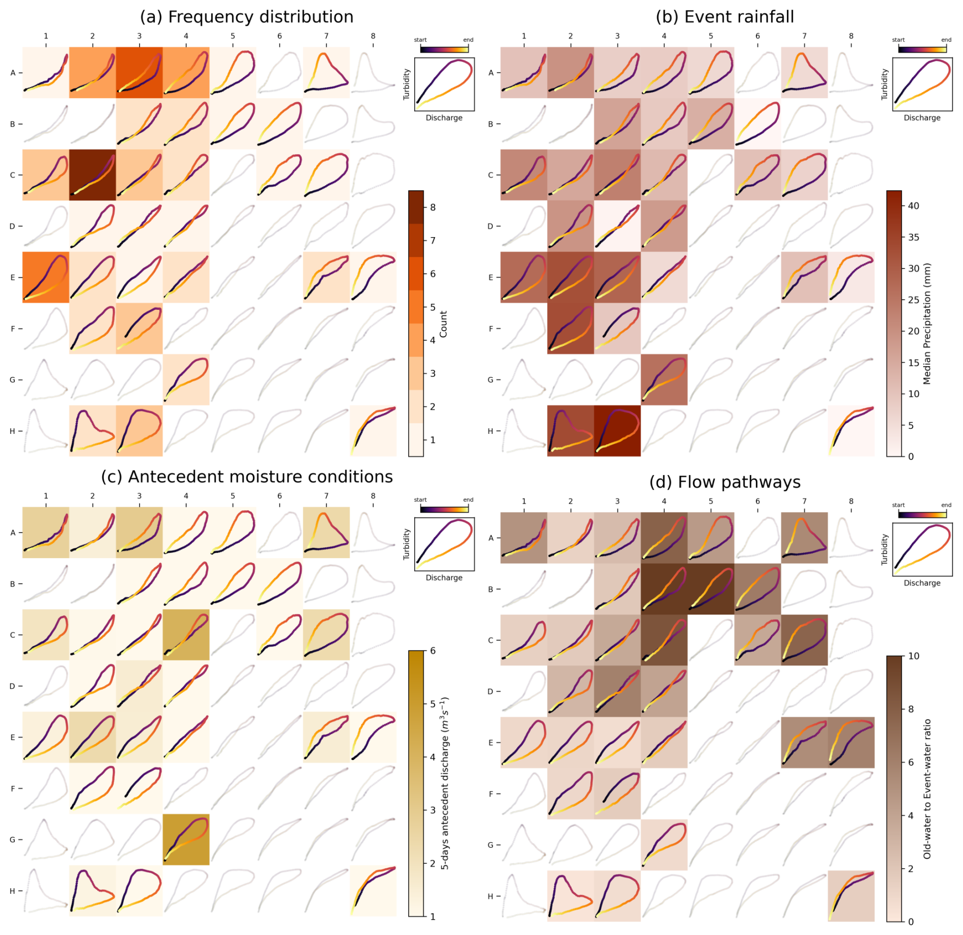
Figure 14 Heatmaps for watershed 03289000 of (a) loop types, (b) precipitation, (c) antecedent discharge, and (d) old-water to event-water ratio. The figure illustrates a visual approach for analyzing associations between hydrologic variables and loop types using the General T–Q SOM. In panels (b) and (c), the color intensity represents the median values of the variable calculated for loop samples mapped to each prototype. Consistent patterns are evident for precipitation (higher precipitation for clockwise loops) and the old-water to event-water ratio (higher ratios for counterclockwise loops), whereas no discernible pattern can be seen for the 5 d antecedent discharge.

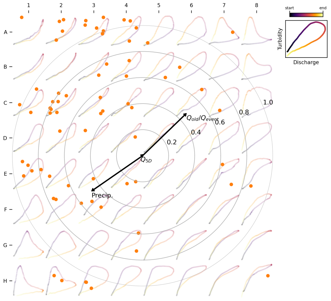
Figure 15 SOM-based biplot. The figure illustrates results from a correlation analysis between hysteresis loop types and hydrologic variables. The direction and length of the arrows are derived from multiple linear correlation analysis, where BMU coordinates serve as the independent variables and the hydrologic variables serve as the dependent variables. Arrows indicate the direction of increasing variable values (e.g., precipitation increases for clockwise loops and decreases for counterclockwise loops). The length of each arrow corresponds to the coefficient of determination for the correlation, with reference values provided by the concentric circles. Each dot represents a sample loop, positioned randomly within the square circumscribed by its respective BMU.

5 Discussion

5.1 Efficacy of the SOM algorithm for C–Q analyses

In this technical note, we introduce a novel approach for characterizing C–Q hysteresis loops using the unsupervised machine learning algorithm, Self-Organizing Maps (SOM). ML has recently proven useful in hysteresis analysis, as demonstrated by Hamshaw et al. (2018), however the application of the SOM algorithm for hysteresis classification overcomes issues associated with classification of hysteresis loops to nominal categories. As discussed in this study, such methods overlook the continuum of hysteresis loop variability by imposing arbitrary boundaries on loop classifications, disregarding the nuanced similarities and differences between loop types (see Fig. 1). In contrast, the SOM-based approach presented here preserves the gradual transitions between hysteresis types, providing a more robust framework for exploring the hydrologic significance of diverse loop types.

Our method also addresses key limitations inherent to hysteresis index-based approaches, which simplify loop shape variability into a single dimension (e.g., clockwise vs. counterclockwise). By contrast, SOMs offer a two-dimensional framework that enables more nuanced discrimination of loop types while maintaining low dimensionality to facilitate further analyses, including visualization (see Figs. 12, 14, and 15). Moreover, the flexibility of this approach allows for extensions into higher dimensions, making it adaptable to the specific requirements of diverse applications.

By applying SOM to a curated dataset of hysteresis loops, representative of sediment transport patterns documented in the literature, we developed the General T–Q SOM. Beyond the advantages over nominal classification schemes, this map also improves upon hysteresis indices by capturing changes in concavity, which is entirely overlooked by traditional hysteresis indices (e.g., Zuecco et al., 2016). Previous studies highlight the importance of concavity in characterizing C–Q relationships. Williams (1989) first described concave up and concave down loops, while Evans and Davies (1998) demonstrated how relative contributions from different flow pathways shape distinct concavity patterns, suggesting concavity as an indicator of constituent sources. Bettel et al. (2025) further reinforced this concept, associating concave up loops with higher base flow contributions. These findings underscore the importance of concavity in understanding C–Q dynamics (see also Fig. 2) and highlight the General T–Q SOM's value in supporting hysteresis workflows, particularly for identifying critical sources and pathways of sediment transport.

5.2 Future use of the SOM algorithm for C–Q analyses

By offering an improved characterization of the spectrum of sediment hysteresis loop types, we believe the SOM algorithm will enhance our understanding of the factors driving their emergence, as illustrated here with the General T–Q SOM. Scaling this analysis across watersheds with diverse physiographic conditions may yield valuable insights into the links between loop types, hydrologic conditions, and watershed characteristics. For example, trained SOMs can be further used to explore seasonal variations in sediment hysteresis within individual watersheds, such as contrasts between wet and dry seasons. Furthermore, the SOM algorithm can support regional or continental-scale characterizations of hysteresis behaviors, enabling comparison of hysteresis patterns across climate zones (e.g., arid and humid basins), as well as different physiographic settings (e.g., flat and steep basins); which, ultimately, may offer critical information to mitigate the negative impacts of excessive sediment transport.

While the General T–Q SOM (Fig. 9) derived herein was created as a proof-of-concept of applying the SOM algorithm for hysteresis analyses, the map can readily be used for sediment transport hysteresis workflows more broadly. We demonstrate how this can be done by using data from three watersheds that were not utilized during the map training process. Importantly, for these watersheds, it was unnecessary to retrain the General T–Q SOM to facilitate the analysis. This trained model is included in the HySOM Python package released with this technical note (see Code and data availability section).

However, studies examining less-common loop patterns or focused on specific loop features may require training alternative T–Q SOMs. For example, Figure-eight loops cannot be reliably distinguished from non-figure-eight loops with similar amplitude and concavity by the General T–Q SOM (see Fig. 10). Attempts to improve the representation of Figure-eight loops (not shown) revealed that including this typology often resulted in highly distorted maps, which compromised the topological structure and disrupted smooth transitions between loop types. We suspect that three- or higher-dimensional SOMs would be a suitable approach for incorporating figure-eight and other loop types while preserving a coherent topological structure in the map. We encourage researchers to explore this alternative.

Furthermore, how to incorporate irregular and less common loops (e.g., watershed-specific loop patterns not represented in the General T–Q SOM) into the SOM framework remains an open area of research. Addressing this challenge, initially, requires identification of loop types that do not fit well with the General T–Q SOM. To identify these events, we propose that two approaches may be employed. For small datasets, visual inspection is recommended to flag loops that deviate fundamentally from those in the General T–Q SOM. This process can leverage the prototype arrangement within the General T–Q SOM to generate a structured visualization of the dataset, as illustrated in the Supplement (Fig. S5). Flagged loops can then be analyzed as an additional category, or the General T–Q SOM could be retrained by incorporating the additional loop type in the training dataset. For larger datasets, where visualization of the entire dataset is impractical, outlier detection methods can be easily implemented for SOMs, for example, by comparing the QE of individual samples with the distribution of QEs for their associated prototypes, as proposed by Munoz and Muruzábal (1998). Interestingly, identified outliers may serve as candidates for training additional SOMs, aiding in the discovery of novel hysteresis patterns. We encourage researchers to use the General T–Q SOM as an initial benchmark and point of comparison to aid with uncovering such patterns in future analyses, thereby facilitating new understanding of the controls of sediment transport in watersheds.

While we chose to curate a dataset containing representative sediment hysteresis patterns for training the General T–Q SOM, alternative methods to train hysteresis SOMs are worth exploring. For example, training on large, uncurated datasets can serve as a powerful exploratory tool, leveraging SOM's visualization strengths to uncover dominant or previously unnoticed loop patterns. Note, however, that less frequent patterns may not be properly captured in the trained SOM due to the learning algorithm's limited exposure to rare types during training (Douzas and Bacao, 2017). Further research is encouraged to develop workflows that better identify and incorporate rare loop types with hydrological relevance.

Similarly, training an SOM on loops from a single watershed may reveal site-specific dynamics and deviations from the General T–Q SOM, offering valuable insights into local hysteresis behavior. However, such watershed-specific SOMs limit comparability across sites, as their prototypes are tailored to a single watershed. Additionally, if the number of available samples is small, the SOM may not be adequately trained, reducing its ability to capture meaningful structure in the hysteresis data.

More broadly, we advocate for developing and carrying out analyses for SOMs tailored to other dissolved and suspended constituents, as distinct loop patterns are likely to emerge for different parameters. For instance, dissolved solids often exhibit dilution during hydrologic events, resulting in loops with a negative overall slope – a pattern rarely seen in sediment transport. To better capture these unique characteristics and understand their controls, we recommend creating C–Q SOM maps for other water quality parameters, such as nutrients, organic carbon, metals, and more. Additionally, researchers may find that distance functions other than DTW better capture hysteresis patterns for certain constituents, and we encourage exploration of such alternatives.

6 Conclusions

This study introduces a novel method for characterizing C–Q hysteresis loops using the Self-Organizing Map (SOM) algorithm. Unlike traditional classification schemes that rely on nominal categories and fail to account for the gradual variability among loop types, the SOM-based framework captures the continuum of hysteresis loop variability. Furthermore, it addresses limitations of hysteresis indices by providing a two-dimensional representation that captures greater detail in loop shapes, offering a more nuanced depiction of the diversity within hysteresis loop types.

Our proof-of-concept application of the SOM algorithm for turbidity-discharge data demonstrates its efficacy for capturing key features of sediment hysteresis loops. This enabled the development of a General T–Q SOM, which represents the primary loop types associated with sediment transport hysteresis patterns. This map characterizes variations in rotational direction, loop amplitude, and, unlike traditional hysteresis indices, loop concavity. The inclusion of concavity adds a critical dimension to hysteresis analysis, as it has been linked to the dominance of different flow pathways, reflecting, along with the rotational direction, the relative contributions of different water and sediment sources. Alternative T–Q SOMs could be developed to better capture loop types not represented by the General T–Q SOM, such as Figure-eight loops or other uncommon patterns. We encourage use of the General T–Q SOM as a benchmark for future studies to facilitate discovery of novel hysteresis patterns.

We demonstrate how the General T–Q SOM can be used to facilitate workflows for hysteresis analysis. For example, we show how the map can be used to visualize hysteresis frequency distributions, facilitate hysteresis comparisons between watersheds, and link hydrologic processes to hysteresis patterns.

Finally, we discuss several promising avenues for application of the SOM algorithm for hysteresis analysis, including discerning seasonality of hysteresis patterns in individual watersheds, and, more broadly, applying the algorithm to characterize hysteresis behavior at the regional or continental scale. We advocate for the development of SOMs tailored to other dissolved and suspended constituents, as distinct loop patterns are likely to emerge for different parameters.