Time shift between precipitation and evaporation has more impact on annual streamflow variability than the elasticity of potential evaporation

One of the most basic questions asked of hydrologists is the quantification of catchment response to climatic variations, i.e., the variations around the average annual flow given the climatic anomaly of a particular year. This paper presents an analysis based on 4122 catchments from four continents, where we investigate how annual streamflow variability depends on climate variables – rainfall and potential evaporation – and on the synchronicity between precipitation and potential evaporation. We use catchment data to verify the existence of this link and show that, in all countries and under the main climates represented, anomalies in this synchronicity are the second most important factor to explain annual streamflow anomalies, after precipitation, but before potential evaporation. Introducing the synchronicity between precipitation and potential evaporation as an independent variable improves the prediction of annual streamflow variability with an average additional explained variance of 6 % globally.

1 Introduction

1.1 On the climate elasticity of streamflow

To assess the impact of climate change on water resources, hydrologists aim to quantify the amount of change in catchment flow when climatic conditions vary. The ratio between changes in streamflow and climate is formally defined as the climate elasticity of streamflow (Schaake and Liu, 1989). The hydrological literature and common sense both suggest that the best factor explaining the changes in annual streamflow is the annual precipitation anomaly (e.g., Pardé, 1933a; Leopold, 1974). In addition, many elasticity studies have also considered the anomaly of potential evaporation, although it is usually only weakly statistically significant in regression studies. In this paper, we focus on a third explanatory variable that quantifies the synchronicity between precipitation and potential evaporation within the year.

1.2 Linear models to predict streamflow anomalies

There is an abundance of literature concerning elasticity studies in hydrology, and our work builds upon the earlier empirical (i.e., measurement-based) studies of Sankarasubramanian et al. (2001), Chiew (2006), and Andréassian et al. (2016). Here, we follow the same principle and use linear regression models based on measured annual data to evaluate the climate elasticity of streamflow. An alternative approach to estimating climate elasticities would involve using hydrological models of varying complexities (e.g., Koster and Suarez, 1999). However, even if models are powerful investigative tools, they also rely on restrictive assumptions that often limit their credibility outside their calibration range. This can be particularly problematic in a large-scale study on the impact of climate change. Thus, we favored an approach introducing the minimal number of hydrological assumptions, hence a linear regression that also has the advantage of being mathematically extremely simple.

1.3 The synchronicity between precipitation and potential evaporation impacts annual streamflow totals

The fact that the time shift between precipitation and potential evaporation, hereon referred to as “climatic synchronicity”, has a hydrological impact has been known for a long time, as shown by a few precursors on this topic. For example, Pardé (1933b) published a classic paper dedicated to the average flow of rivers, where he underlined that “for identical values of precipitation and temperature, everything else being equal, the runoff coefficient $Q/P$ will be smaller where the larger part of precipitation falls during the warm season”. Similarly, Coutagne and de Martonne (1935) discussed formulas for annual streamflow, and underlined that formulas based only on the humidity ratio $P/E_{\mathrm{0}}$ are deficient, because they fail to account for “the distribution of precipitations between seasons, in particular, in the temperate zone, between the warm and the cold season. Of two years of equal precipitation, the year which will receive the most part in summer will produce the less annual flow”. Additional classical studies include Thornthwaite (1948), who proposed to classify climates initially with two indices (one characterizing the periods of water surplus and the other the periods of water deficiency), which he subsequently combined into a single index. A few years later, Turc (1954) introduced his famous formula for long-term actual evaporation. At the very end of his paper, he wrote that “the most urgent improvement” to his actual evaporation formula should be the introduction of the “distribution of precipitations and of the temperature changes within the year.”

Recent studies have also discussed the impact of climate seasonality on water balance, based on either theoretical or empirical approaches. Among the theoretical studies, Dooge (1992) presented catchment yield curves where he introduced as a parameter the length of the dry season. Milly (1994) proposed a theoretical computation of actual evaporation based on the seasonality of the aridity index. Yokoo et al. (2008) made theoretical computations on the difference between in-phase and out-of-phase regimes of precipitation and potential evapotranspiration. Additionally, Roderick and Farquhar (2011), Feng et al. (2012), Donohue et al. (2012), Berghuijs et al. (2014) and Jawitz et al. (2022) all made notable developments. Among the empirical studies, Potter et al. (2005) quantified the impact of rainfall seasonality on mean annual water balance in Australia. Hickel and Zhang (2006) discussed the antagonistic effects of climate seasonality and soil moisture storage. More recently, de Lavenne and Andréassian (2018) proposed a synchronicity index to characterize the phase difference between precipitation and potential evaporation, and Feng et al. (2019) proposed an index of asynchronicity for Mediterranean climates.

1.4 Purpose of the paper

In this paper, we aim to improve the prediction of streamflow elasticity by introducing anomalies in synchronicity between precipitation and potential evaporation as a predictor, alongside variability in rainfall and potential evapotranspiration. Our study is based solely on data analysis, and uses only linear regression models.

2 Test catchments

2.1 Origin of the dataset

As presented in Table 1, we use catchments from nine countries to base our analysis on a wide range of climates.

Table 1 Origin of the catchments used in this paper.

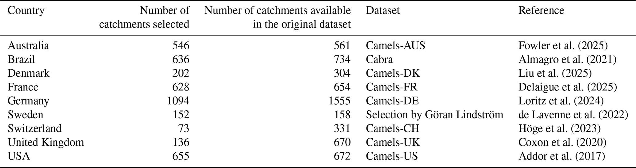
The total number of catchments is 4122, for a total of 162 005 station-years (the average length of catchment time series is 39 years). We use hydrological years as defined in the Notations section.

2.2 Catchment selection

The catchments used in this paper were selected from several datasets indicated in Table 1 and represent approximately 75 % of the original catchments. Our catchment selection was based on three criteria: record length, catchment memory and regulation degree. First, we only selected catchments that had more than 20 complete hydrological years. Second, we selected catchments that exhibit minimal interannual memory (“memory” as defined by de Lavenne et al., 2022). This criterion was needed because the equation used here to estimate streamflow elasticity is only hydrologically warranted for catchments displaying minimum interannual memory, thus allowing a straightforward computation of annual elasticity coefficients, based only on annual average values. Finally, catchments identified as significantly regulated by reservoirs were removed. This identification was done by either asking the datasets authors, or, where the information was available, by setting a limit equal to 10 mm equivalent volume storage in dams). For Switzerland, the list of almost natural catchments published by Muelchi et al. (2022) was utilized.

2.3 Climatic inputs

Where several precipitation products were available in the original dataset, we used the product recommended by dataset authors as being of the best quality, while avoiding precipitation data based exclusively on satellite estimates.

In the original datasets, potential evaporation was computed with a variety of different formulas (Makkink, Morton, FAO-56, Penman-Monteith, Hargreaves, Oudin, etc.). For the sake of homogeneity, we recomputed it (at the daily time step) for all catchments using the formula proposed by Oudin et al. (2005), which requires only extraterrestrial radiation and air temperature. This formula was selected for two reasons: first, it could be computed, given the available data, for all datasets, and it has been widely used worldwide and appears appropriate (while of course not perfect) for describing atmospheric evaporative demand.

2.4 Characteristics of the catchment set

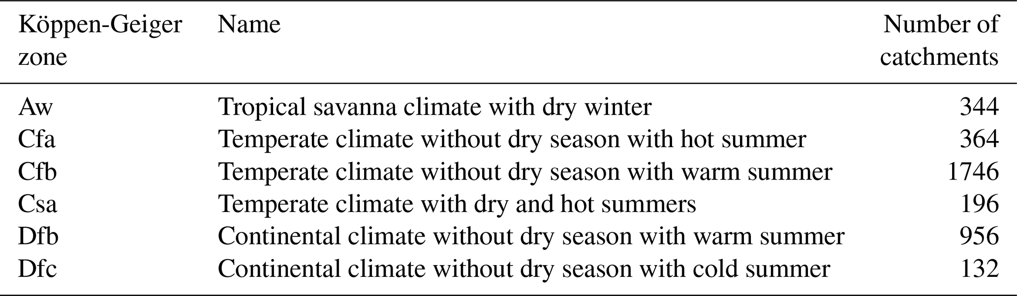
In our dataset, the aridity index, computed as $E_{\mathrm{0}}/P$, ranges from 0.1 to 6.3, with a first quartile of 0.6 and a third quartile of 1.0. The mean and the median of the aridity index are both 0.8. In order to assess the generality of the results, we will discuss them at the country scale and also by climatic classes following the Köppen-Geiger classification (see e.g., Peel et al. 2007 and Table 2). Note that we only give numerical results for the climatic zones with more than 100 catchments.

Table 2 Main climatic zones (in the sense of the Köppen-Geiger classification) represented in our dataset (we present the zones counting more than 100 catchments).

Finally, Fig. 1 presents the 4122 catchments of our dataset with two variants of the Turc-Budyko non-dimensional graph. On the left-hand graph, each catchment corresponds to one point, with coordinates representing the average aridity on the x-axis and “actual evaporation” yield, computed as $(P-Q)/P$, on the y-axis. On the right-hand graph, each catchment is represented by a single point, with coordinates indicating the average humidity on the x-axis and the average streamflow yield, computed as $Q/P$, on the y-axis.

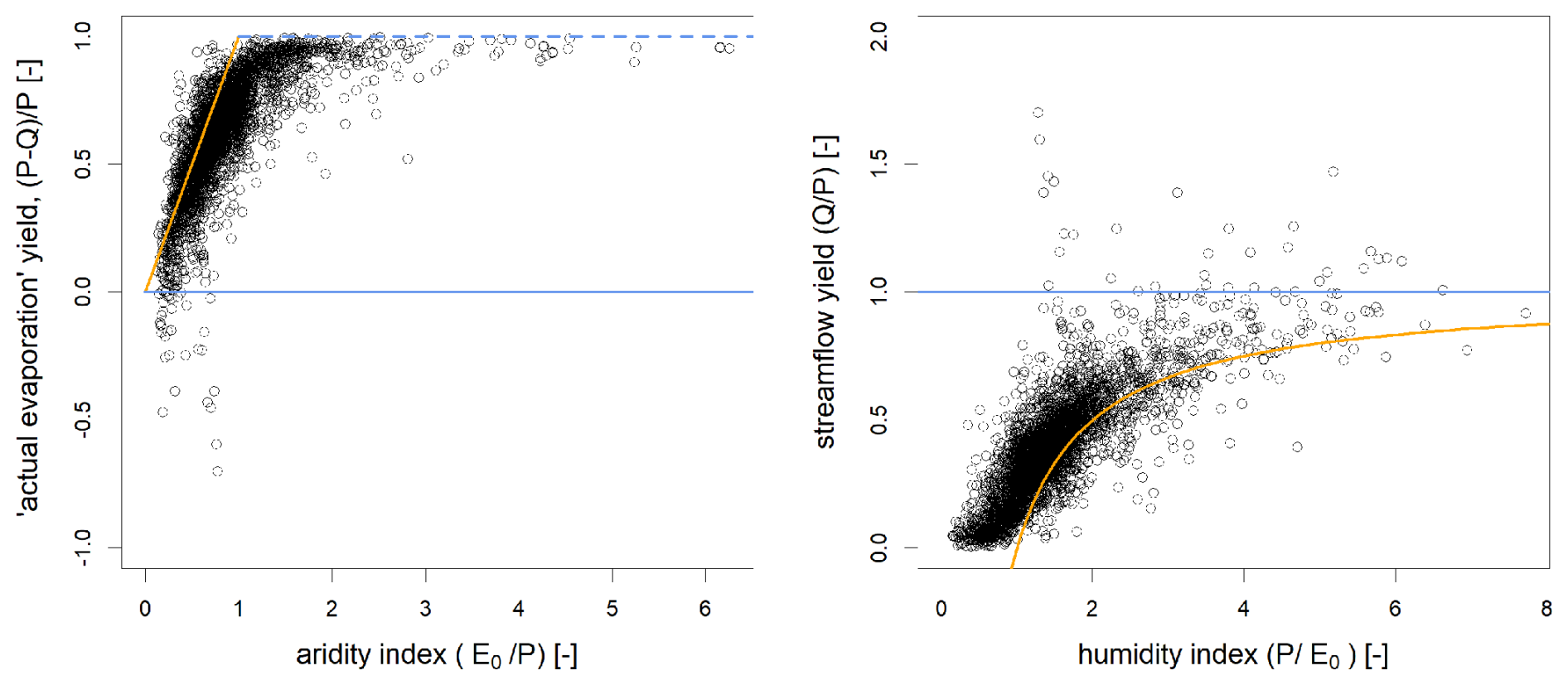
Figure 1 Representation of the 4122 catchments in two equivalent forms of the Turc-Budyko non-dimensional space. The solid blue line corresponds to the water limit (Q=P), and the orange line corresponds to the energy limit ($Q=P-E_{\mathrm{0}}$). On the left, an additional limit (dotted blue line) is sometimes improperly referred to as “water limit” in the literature, but it only corresponds to the physical limit (Q=0, when one estimates the actual evaporation as the difference between discharge and precipitation. The catchments that are beyond the orange line (i.e., above on the left and below on the right) are “leaky” (in the sense that they contribute to the recharge of a regional aquifer) and those which are beyond the blue line (i.e., below on the left and above on the right) are “gaining” in the sense of a karstic catchment which would drain a larger than specified catchment (note that in a few cases, data uncertainties might also cause catchments to be beyond the limits).

3 Method

3.1 Computation of the synchronicity of precipitation and potential evaporation

In this paper, we utilize a modified version of the seasonality index introduced by de Lavenne and Andréassian (2018): a detailed discussion of the reasons for this change is provided in Appendix A. The objective of this index (Λ) is to characterize the synchronicity between precipitation P and potential evaporation E₀ at the annual time step. For each year n, we define the part of annual precipitation that is the most easily accessible to evaporation (i.e., neutralizable by evaporation) as in Eq. (1) and Fig. 2:

$$\begin{array}{}\text{(1)}& \mathrm{\text{synchronous}}P-E_{\mathrm{0}}\text{amount}={\sum }_{m=\mathrm{1}}^{\mathrm{12}}min\left(P_{m,n},E_{{\mathrm{0}}_{m,n}}\right)\end{array}$$

where the index m refers to the calendar month.

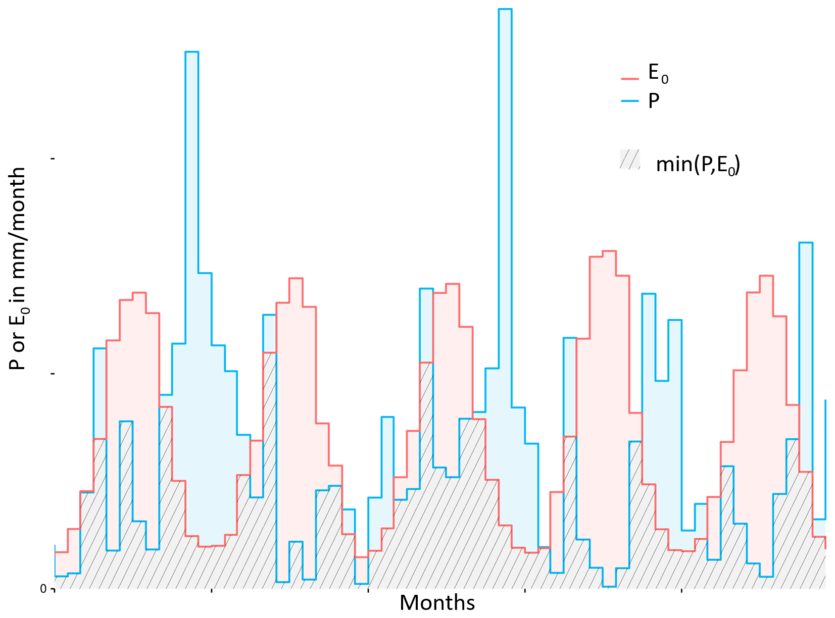
Figure 2 Two series of precipitation and potential evaporation at catchment scale: the part of precipitation that is the most easily accessible to evaporation is illustrated in hatched pattern.

The percentage of easily neutralizable precipitation is then defined as Eq. (2), and the percentage of easily neutralizable potential evaporation as Eq. (3).

$$\begin{array}{}\text{(2)}& {\displaystyle }{\mathit{\lambda }}_{\mathrm{1},n}={\displaystyle \frac{{\sum }_{m=\mathrm{1}}^{\mathrm{12}}min\left(P_{m,n},E_{{\mathrm{0}}_{m,n}}\right)}{P_n}}\text{(3)}& {\displaystyle }{\mathit{\lambda }}_{\mathrm{2},n}={\displaystyle \frac{{\sum }_{m=\mathrm{1}}^{\mathrm{12}}min\left(P_{m,n},E_{{\mathrm{0}}_{m,n}}\right)}{E_{{\mathrm{0}}_n}}}\end{array}$$

Because both ratios belong to the interval [0,1], their geometric average will also be within the same range (Eq. 4).

$$\begin{array}{}\text{(4)}& {\mathit{\lambda }}_{\mathrm{3},n}=\sqrt{{\mathit{\lambda }}_{\mathrm{1},n}{\mathit{\lambda }}_{\mathrm{2},n}}={\displaystyle \frac{{\sum }_{m=\mathrm{1}}^{\mathrm{12}}min\left(P_{m,n},E_{{\mathrm{0}}_{m,n}}\right)}{\sqrt{P_n{E}_{{\mathrm{0}}_n}}}}\end{array}$$

Finally, the index Λ rescales and combines λ₁ and λ₂ into a single quantity, expressed in mm yr⁻¹, representing the average ratio of neutralizable precipitation and neutralizable potential evaporation as shown in Eq. (5). For two years with the same annual amounts of precipitation and potential evaporation, Λ will reach higher values when P and E₀ are synchronous, and lower values when they are out of phase.

$$\begin{array}{}\text{(5)}& {\mathrm{\Lambda }}_n={\mathit{\lambda }}_{\mathrm{3},n}\cdot \overline{P}={\displaystyle \frac{{\sum }_{m=\mathrm{1}}^{\mathrm{12}}min\left(P_{m,n},E_{{\mathrm{0}}_{m,n}}\right)}{\sqrt{P_n\cdot E_{{\mathrm{0}}_n}}}}\cdot \overline{P}\end{array}$$

3.2 Computation of streamflow elasticities

To compute the streamflow elasticities, we solve two linear equations given by Eqs. (6) and (7).

$$\begin{array}{}\text{(6)}& {\displaystyle }\mathrm{\Delta }{Q}_n=e_{Q/P}\mathrm{\Delta }{P}_n+e_{Q/E_{\mathrm{0}}}\mathrm{\Delta }{E}_{{\mathrm{0}}_n}\text{(7)}& {\displaystyle }\mathrm{\Delta }{Q}_n=e_{Q/P}\mathrm{\Delta }{P}_n+e_{Q/E_{\mathrm{0}}}\mathrm{\Delta }{E}_{{\mathrm{0}}_n}+e_{Q/\mathrm{\Lambda }}\mathrm{\Delta }{\mathrm{\Lambda }}_n\end{array}$$

Where ΔQ_n (respectively ΔP_n, $\mathrm{\Delta }{E}_{{\mathrm{0}}_n}$, ΔΛ_n) represents the deviation from the mean annual value (anomaly) for variable Q (respectively P, E₀, Λ) in mm yr⁻¹ and $e_{Q/P}$, $e_{Q/E_{\mathrm{0}}}$ and $e_{Q/\mathrm{\Lambda }}$ represent the elasticity of streamflow with respect to P, E₀, and Λ(dimensionless).

Equation (6) represents the classical approach to elasticity computation (Andréassian et al., 2016), while Eq. (7) represents the original contribution of this paper, and aims at determining how far climatic synchronicity explains annual streamflow variability.

The elasticities in Eqs. (6) and (7) are estimated via ordinary least squares (OLS). More complex statistical models such as generalized least squares are not required because the selected catchments do not exhibit interannual memory, as explained in the data section. This absence of interannual memory guarantees the lack of autocorrelation in annual streamflow, which is an important statistical assumption for OLS. Additionally, we chose a p-value threshold of 0.05 for all the discussion of results. We compute elasticity coefficients between anomalies of equal dimensions (in mm yr⁻¹), and not between relative anomalies (in %) because with the anomalies expressed in mm yr⁻¹ the physically-plausible range is known: [0,1] for $e_{Q/P}$, [−1,0] for $e_{Q/E_{\mathrm{0}}}$ and $e_{Q/\mathrm{\Lambda }}$. Finally, Eqs. (6) and (7) were solved on a catchment-by-catchment basis, i.e., we computed 4122 distinct regressions.

Figure 3 illustrates this catchment-based computation using the example of the Meurthe River at Raon-l'Étape (727 km²). For this catchment, annual streamflow anomalies exhibit a well-defined dependency on both precipitation and synchronicity anomalies, with the dependency on potential evaporation anomaly being very weak.

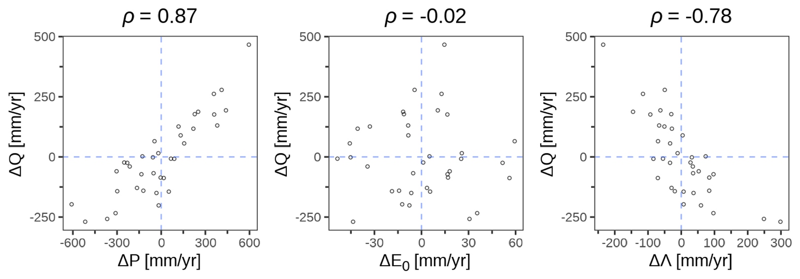
Figure 3 Example of an elasticity plot for the Meurthe River at Raon-l'Étape (A615103001): each point corresponds to one hydrological year (for this catchment, 36 hydrological years were available, from 1975 to 2021). The Pearson correlations of ΔQ with ΔP, ΔE₀ and ΔΛ are respectively 0.87, −0.02 and −0.78.

The visual impression of Fig. 3 is confirmed by the results of the linear regressions of Eqs. (6) and (7) in Table 3. Values of the Student's t-test indicate that precipitation has a dominant contribution, while the contribution of potential evaporation is not statistically significant. The introduction of synchronicity increases the R² from 0.75 to 0.80.

Table 3 Climate elasticity coefficients computed with and without the inclusion of the synchronicity variable Λ for the example catchment (La Meurthe at Raon-l'Étape).

4 Results

4.1 Graphical analysis of anomalies by country

To provide a general overview of the correlation between streamflow anomalies and climatic anomalies, Figs. 4 and 5 present an aggregated plot for each country and for each main climate class, combining the anomalies of all catchments. At this scale, only general trends are apparent. As expected, streamflow anomaly is clearly positively correlated with precipitation anomaly in all countries; streamflow anomaly is, overall, very weakly negatively correlated with potential evaporation anomaly, Denmark being the only outlier with a weak positive correlation (it is mainly due to the year 1990, which was a very dry year in Denmark, but with an unusual cold summer). Streamflow anomaly is clearly negatively correlated to the synchronicity index anomaly (Λ) for all countries. This negative correlation indicates that years with a lower Λ (i.e., when precipitation and potential evaporation are more out of phase) yield greater streamflow. This observation is perfectly hydro-logical, and conforms to general observations previously identified by Pardé (1933a). In the case of Australia, where streamflow anomalies are clearly negatively correlated to the synchronicity index anomaly (Λ) on Fig. 4, it is interesting to mention the opposite conclusion of Potter et al. (2005) who wrote that “the inclusion of seasonally varying forcing alone was not sufficient to explain variability in the mean annual water balance”. This surprising conclusion may be an artefact of the index chosen by the authors to describe seasonality.

Overall, the most surprising fact is that streamflow anomaly appears more strongly correlated with the synchronicity index anomaly than with the potential evaporation anomaly.

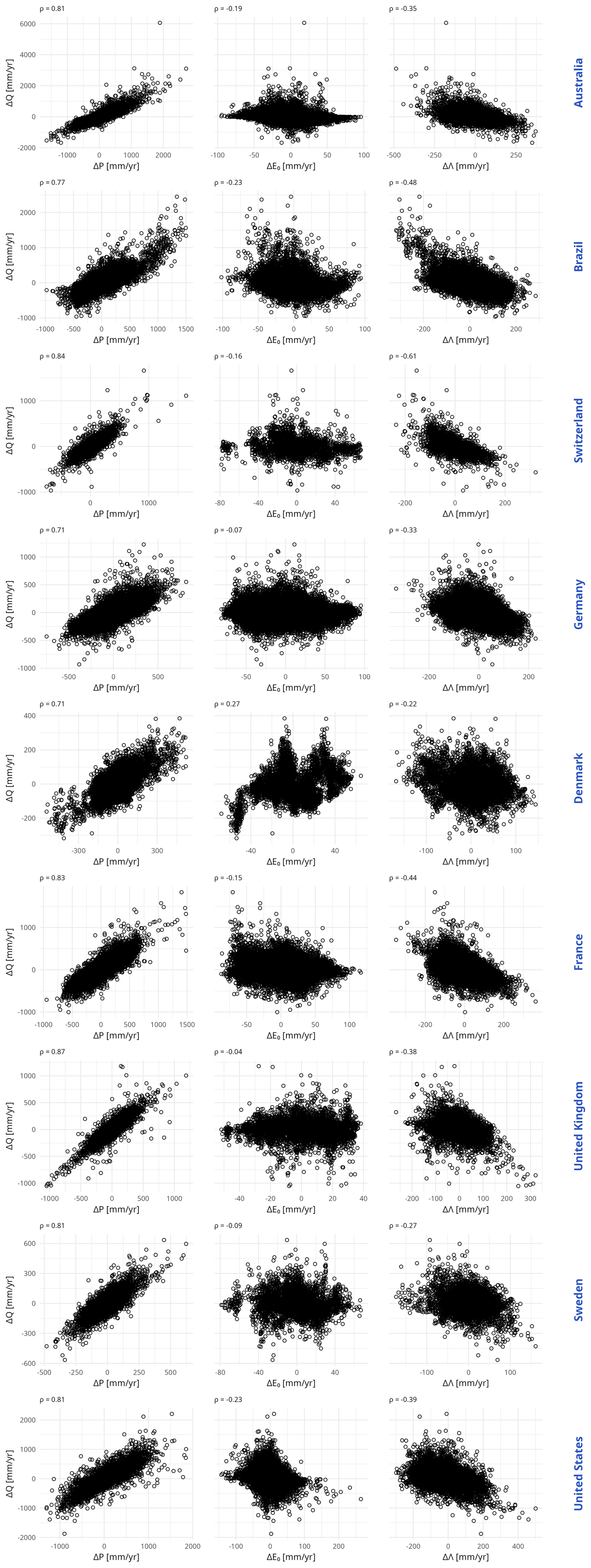
Figure 4 Scatter plots, for each country, between streamflow anomalies ΔQ, and: precipitation anomalies ΔP (left), potential evaporation anomalies ΔE₀ (middle) and synchronicity index anomalies ΔΛ (right). Each point represents one station-year. Above each scatter plot, we provide the corresponding Pearson correlation.

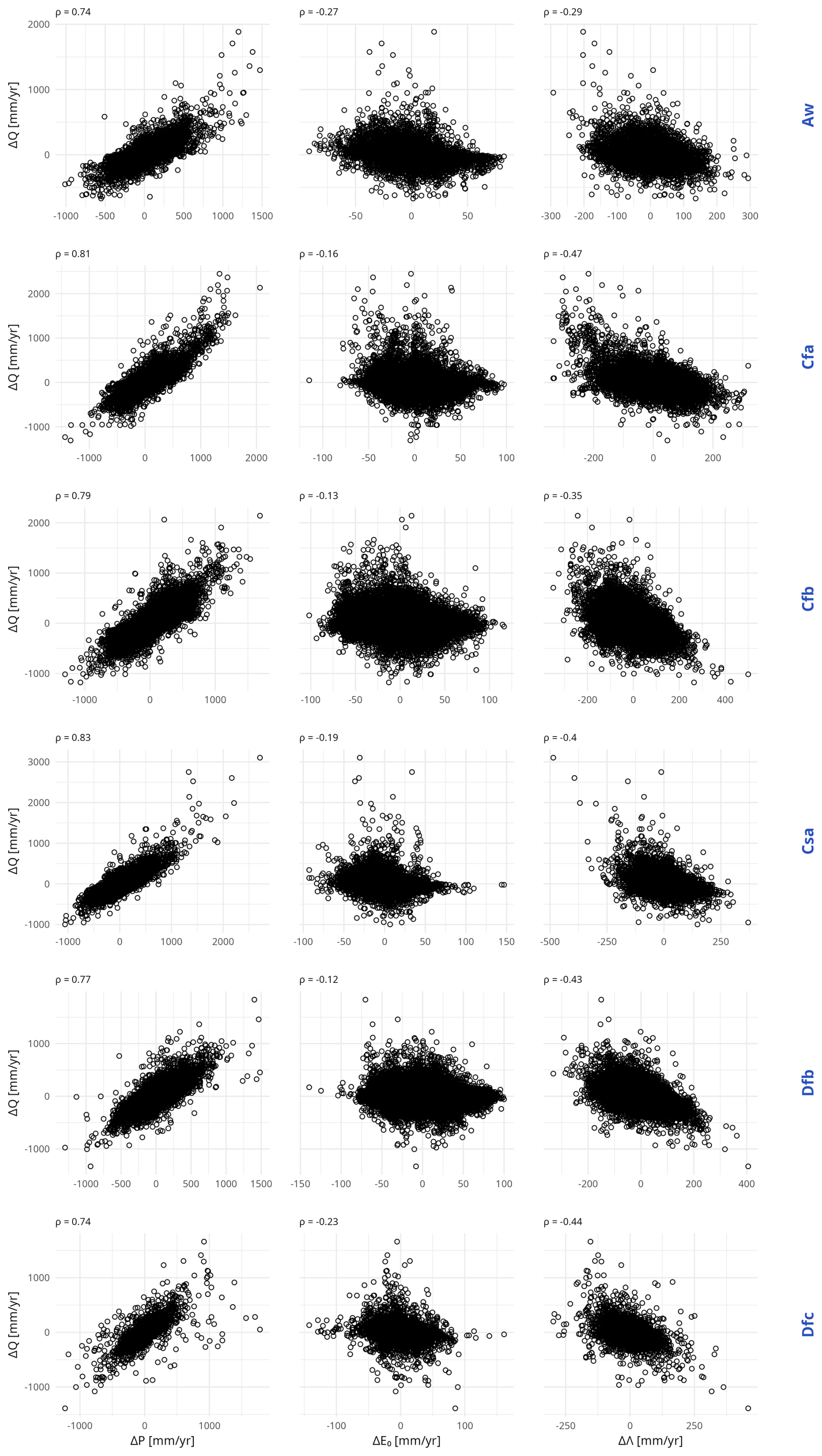
Figure 5 Scatter plots, for the main climate classes, between streamflow anomalies ΔQ, and: precipitation anomalies ΔP (left), potential evaporation anomalies ΔE₀ (middle) and synchronicity index anomalies ΔΛ (right). Each point represents one station-year. Above each scatter plot, we provide the corresponding Pearson correlation.

4.2 Overall results by catchment

We now analyze the results obtained for each of the 4122 catchments. Table 4 shows the statistics of the individual regressions for the classical case when synchronicity is not included as a predictor. This analysis reveals that for all countries and all climate groups, the precipitation elasticity of streamflow is almost always significant at the 0.05 level. On the other hand, the potential evaporation elasticity of streamflow is not frequently significant at the 0.05 level. In addition, the regression identifies physically realistic precipitation elasticity values (between 0 and 1) for almost all catchments (93 % worldwide, and a minimum of 80 % across different groupings), whereas potential evapotranspiration elasticity is frequently physically unrealistic with only 6 % of values in the range [0,1] globally.

Table 4 Linear regression results by country and climate type for Eq. (6) when regression uses two independent variables P and E₀ to explain streamflow anomaly.

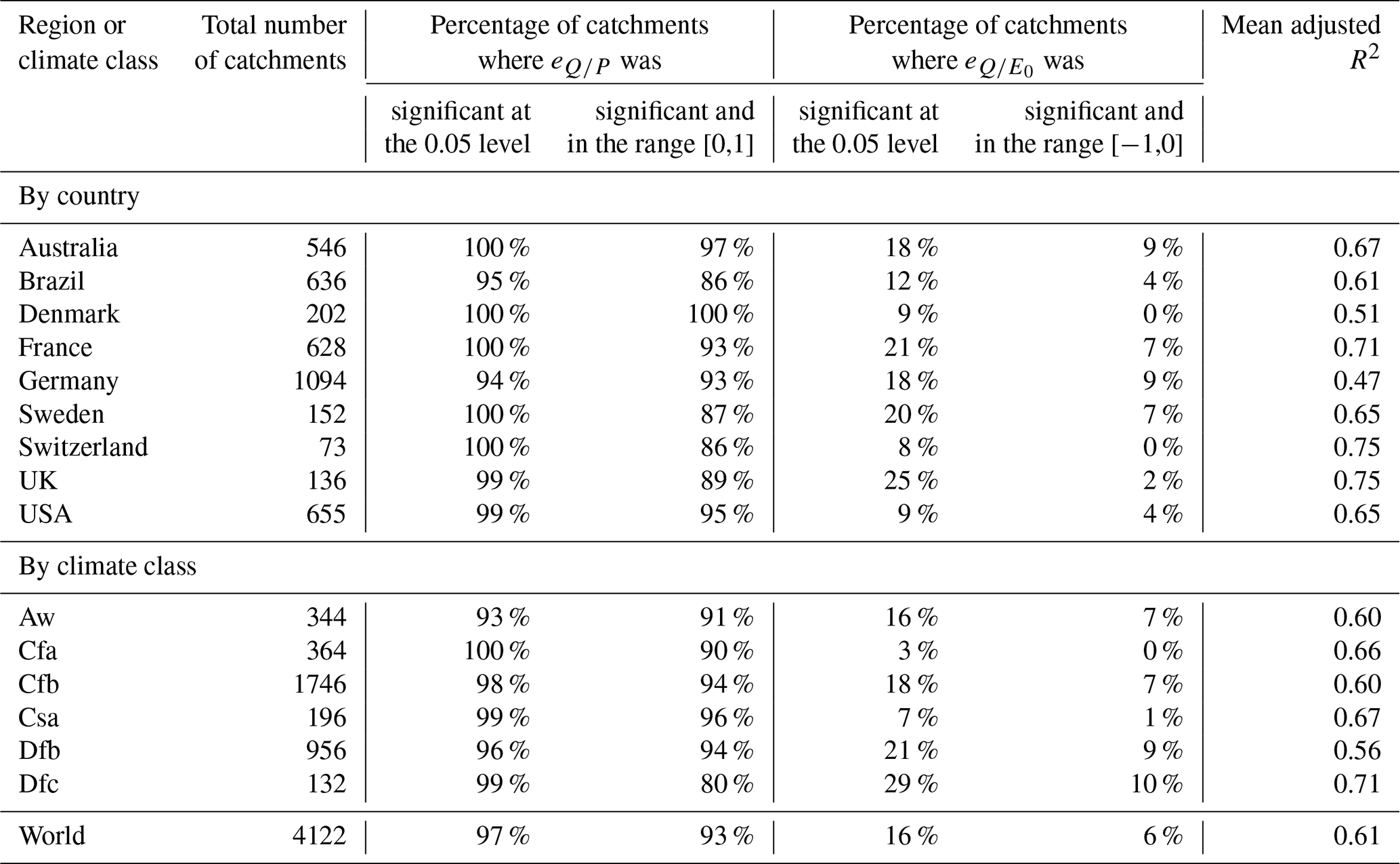
Aw – Tropical savanna climate with dry winter, Cfa – Temperate climate without dry season with hot summer, Cfb – Temperate climate without dry season with warm summer, Csa – Temperate climate with dry and hot summers, Dfb – Continental climate without dry season with warm summer, Dfc – Continental climate without dry season with cold summer

Table 5 presents the same statistics, when the synchronicity anomaly (ΔΛ_n) is introduced into the elasticity regression (Eq. 7). This analysis shows that the average efficiency of the regression equation increases across all countries and climate groups (see also Fig. 6). While an increase is expected when an additional predictor is added to a regression, please note that we are presenting adjusted R² values, which are designed to take that issue into account. The average additional explained variance lies in the range 3 %–10 % (6 % globally), depending on the group, and we consider it a noticeable improvement. Additionally, the synchronicity anomaly (ΔΛ_n) provides a significant contribution to the regression for 64 % of the catchments, compared to only 23 % for potential evaporation).

More important, the introduction of the synchronicity anomaly (ΔΛ_n) does not modify the significance of the other two elasticity coefficients $e_{Q/P}$ and $e_{Q/E_{\mathrm{0}}}$. A slight increase is observed in the proportion of catchments where $e_{Q/E_{\mathrm{0}}}$ coefficient is significant at the 0.05 level (from 16 % to 23 %). Moreover, the utilization of ΔΛ_n does not degrade the physical realism of the elasticity coefficients $e_{Q/P}$ and $e_{Q/E_{\mathrm{0}}}$. Once again, a slight increase is observed in the proportion of catchments where $e_{Q/P}$ coefficient is significant and in the physical range [0,1] (from 93 % to 94 %), and where $e_{Q/E_{\mathrm{0}}}$ coefficient is significant at the 0.05 level and in the physical range [−1,0] (from 6 % to 11 %). Finally, only two countries (Switzerland and Brazil) and one climate type (Dfc – Continental climate without dry season with cold summer) showed lower relevance of the synchronicity index compared to other regions. We attribute this reduced relevance in Switzerland and climate zone Dfc to the essentially energy-limited nature of the catchments as our selection criteria for Switzerland prioritized high-elevation catchments with minimal anthropogenic impact (see also the Discussion section and Fig. 9). Last, note that in all groupings except Dfc, the number of catchments where $e_{Q/\mathrm{\Lambda }}$ is significant at the 0.05 level exceeds that where the $e_{Q/E_{\mathrm{0}}}$ coefficient is significant at the same level.

Table 5 Linear regression results by country and climate type for Eq. (7) when regression uses three independent variables to explain streamflow anomaly (to allow for comparison, the last column reports the mean R² of Table 4).

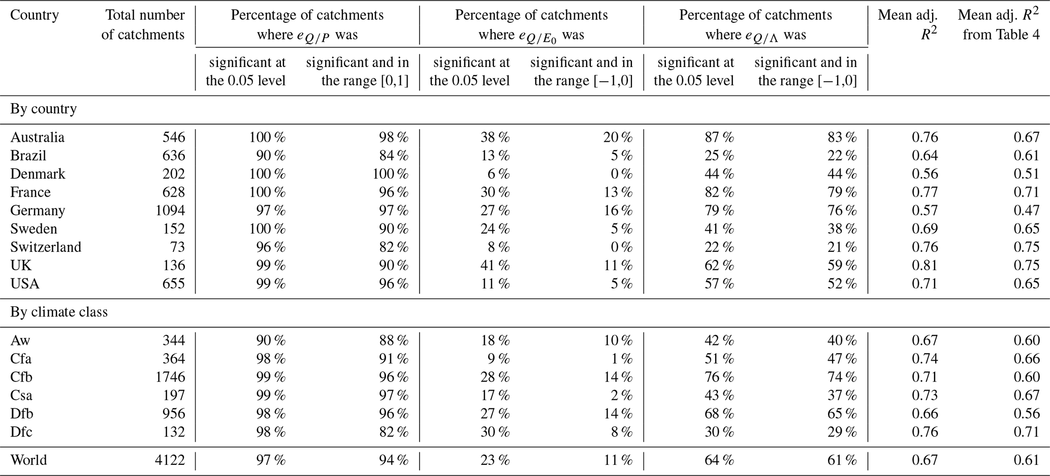
Aw – Tropical savanna climate with dry winter, Cfa – Temperate climate without dry season with hot summer, Cfb – Temperate climate without dry season with warm summer, Csa – Temperate climate with dry and hot summers, Dfb – Continental climate without dry season with warm summer, Dfc – Continental climate without dry season with cold summer

5 Discussion

Figure 6 illustrates the improvement in explanatory capacity of the regressions due to the introduction of the synchronicity anomalies. While considerable variability exists, and some catchments show equivalent performance between the two regression models (indicated by points on the 1:1 line), the graph confirms that for many catchments (approximately 66  % of the dataset, where $e_{Q/\mathrm{\Lambda }}$ was significant at the 0.05 level), accounting for synchronicity anomalies visibly improves the efficiency of the linear regression. Because the adjusted R² shows the same trend as the classical R², this is clearly not a simple effect of the increase of independent variables in the regression.

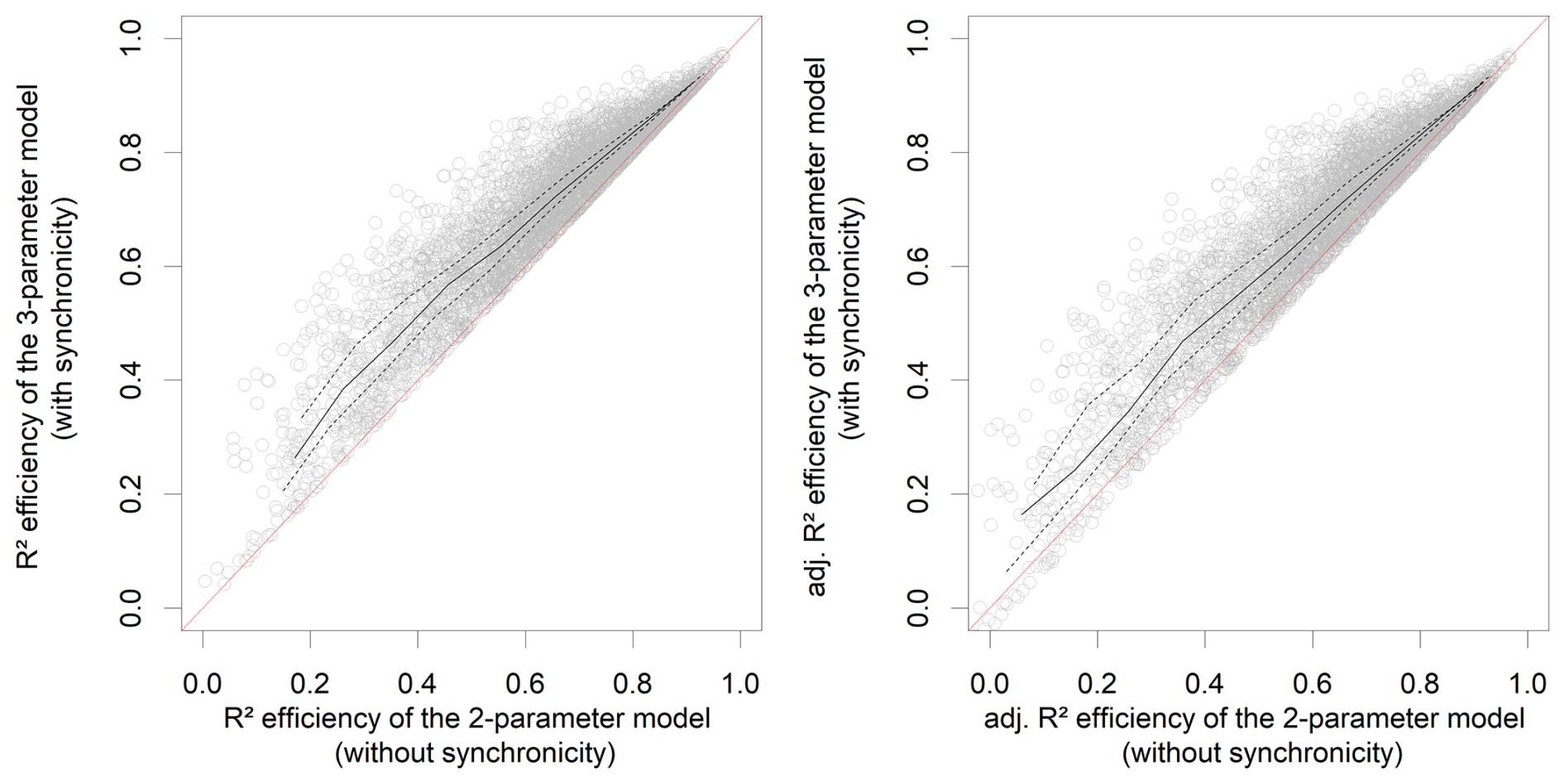
Figure 6 Comparison of the performances of the 2-parameter streamflow elasticity model (Eq. 6, which does not account for P−E₀ synchronicity) and the 3-parameter model (Eq. 7, which does). Each point represents one of the 4122 catchments of our dataset. The solid line represents the median, and the dashed lines represent the first and the third quartiles. As measure of efficiency, we use the R² on the left plot and the adjusted R² on the right one.

In Fig. 7, we summarize the significance of the $e_{Q/\mathrm{\Lambda }}$ coefficient across all the Köppen climate classes represented in our dataset: $e_{Q/\mathrm{\Lambda }}$ is significant at the 0.05 level for 50 % of the catchments in 11 classes (representing 79 % of the catchments).

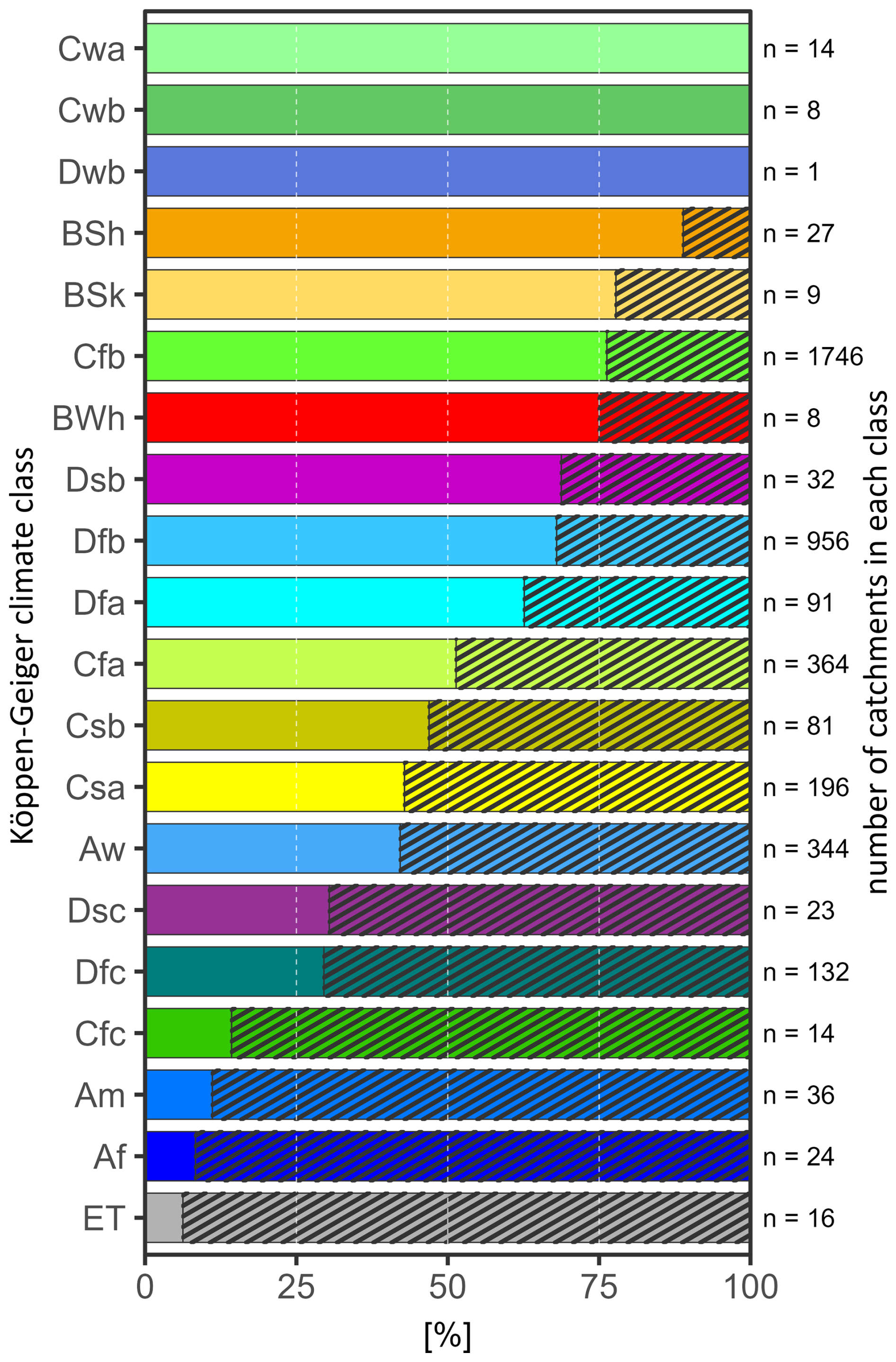
Figure 7 Significance of the P−E₀ synchronicity anomalies by Köppen climate class: the dashed area represents the proportion of catchments for which synchronicity was not deemed significant.

Figure 8 shows the geographic distribution of the catchments where the P−E₀ synchronicity had a significant contribution to explain streamflow anomalies (with a p-value threshold of 0.05). The map brings further elements to Table 5 and illustrates that there are sub-regions where the coefficient $e_{Q/\mathrm{\Lambda }}$ is mostly not significant at the 0.05 level. Based on our knowledge of the climatic specificities of each country, this seems to be possibly correlated to higher rainfall (cf. the Danish dataset, with the particular behavior of the West of Jutland, the case of Florida in the US, the case of the Scottish catchments in Great Britain) and/or to colder areas (cf. the Swiss, Swedish and US datasets).

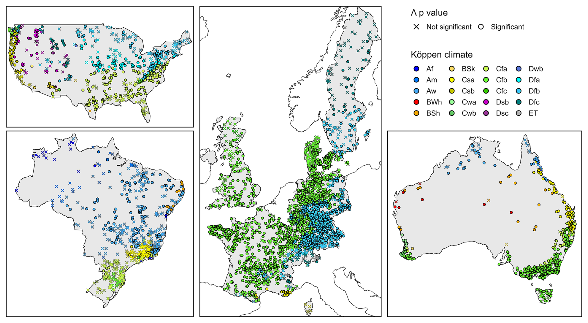
Figure 8 Map of the 4122 catchments used in this study, each catchment is represented by either a circle (where the P−E₀ synchronicity anomalies had a significant contribution to explain streamflow anomalies) or a cross (where it was not significant at the 0.05 level). The color of circles and crosses corresponds to the Köppen climate classes.

To verify this hypothesis, Fig. 9 presents the p-values of the 4122 e_Q.Λ coefficients as a function of the humidity index $P/E_{\mathrm{0}}$. This graph clearly indicates that most of the humid catchments (Humidity index > 2) lack sensitivity to the P−E₀ seasonality, and this pattern is likely the main explanation for the geographical patterns observed in Fig. 8.

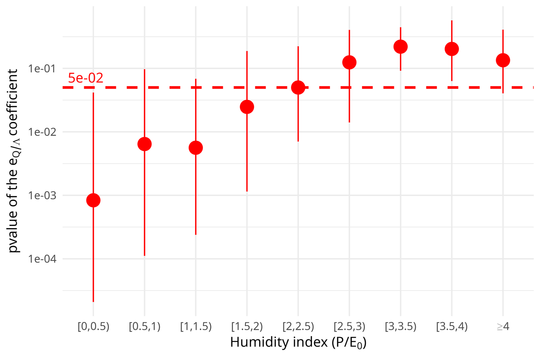
Figure 9 Distribution of the p-values of the 4122 $e_{Q/\mathrm{\Lambda }}$ coefficients as a function of the humidity index $P/E_{\mathrm{0}}$. The red points represent the median, the bar represent the interquartile range, and the dashed line represents the 0.05 threshold.

6 Conclusions

6.1 Synthesis

In this paper, we investigated the dependency between streamflow elasticity and the synchronicity of precipitation and potential evaporation, using a dataset of 4122 catchments located in Europe, Australia, North America and South America. Our analysis provided three main findings. First, we empirically verified the strong correlation among streamflow anomalies, annual precipitation anomalies, and synchronous P−E₀ anomalies. Second, we demonstrated that the role of the synchronicity between P and E₀ in explaining streamflow anomalies is significantly more important than that of E₀ anomalies. Finally, we showed that introducing synchronicity between precipitation and potential evaporation as an additional predictor in the linear regression clearly improves the prediction of annual streamflow variability.

6.2 Perspectives

Notwithstanding these positive results, some estimated elasticity values remain outside of their physically acceptable domain (i.e., [0,1] for $e_{Q/P}$ and [−1,0] for $e_{Q/E_{\mathrm{0}}}$ and $e_{Q/\mathrm{\Lambda }}$). For precipitation elasticity ($e_{Q/P}$), 93 % of the catchments were within the physical range, out of a total of 97 % where precipitation elasticity was significant. For potential evaporation elasticity ($e_{Q/E_{\mathrm{0}}}$), a lack of physical realism occurs in most of the cases (i.e., only 11 % of the catchments were within the physical range, out of a total of 23 % where potential evaporation elasticity was significant). This is very likely due to a sensitivity problem in the regression, which contributes to the difficulty in obtaining realistic elasticity coefficients. Finally, for synchronicity elasticity ($e_{Q/\mathrm{\Lambda }}$), 61 % of the catchments were within the physical range out of a total of 64 % where synchronicity elasticity was significant. In the future, we aim to investigate alternative statistical models that could better constrain the elasticity coefficients within their physically realistic domain.

Appendix A: Further details to justify our choice for the synchronicity index

There is no unique solution for choosing a measure of synchronicity between Precipitation and Potential Evaporation. In a previous paper (de Lavenne and Andréassian, 2018) we presented a non-dimensional index (λ), defined as follows (A1):

$$\begin{array}{}\text{(A1)}& \mathit{\lambda }={\displaystyle \frac{{\sum }_{m=\mathrm{1}}^{\mathrm{12}}min\left(P_{m,n},E_{{\mathrm{0}}_{m,n}}\right)}{{\sum }_{m=\mathrm{1}}^{\mathrm{12}}max\left(P_{m,n},E_{{\mathrm{0}}_{m,n}}\right)}}\end{array}$$

A reviewer of this paper remarked that our interpretation of this index did not hold in extreme cases. Thus, we modified it in order to improve its interpretability. We also tried to replace it with simpler versions, and we would like to present these alternatives in order to save time and effort for those who would like to keep working on this topic.

The first simplification which was tested (called here S1) consisted in using directly the synchronous P−E₀ amount:

$$\begin{array}{}\text{(A2)}& S\mathrm{1}\left(n\right)={\sum }_{m=\mathrm{1}}^{\mathrm{12}}min\left(P_{m,n},E_{{\mathrm{0}}_{m,n}}\right)\end{array}$$

S1 was an interesting solution because it yielded directly a value in mm yr⁻¹, without the need for rescaling, and it clearly represented the precipitation volume that was the most easily accessible to evaporation. In the linear regression, it did give very high average adjusted R² (world average of 0.67, the same as for the solution retained). The reason why we did not consider this solution was that there was a correlation between ΔS1 and ΔP for many catchments (average correlation of +0.58 over the 4122 catchments, reaching +0.74 over the Australian catchments), and introducing two correlated variables in a regression equation is clearly bad statistical practice.

To avoid this high correlation, we tested a normalization using annual precipitation, which we redimensionalized using the average interannual precipitation as in Eq. (A3) below:

$$\begin{array}{}\text{(A3)}& S\mathrm{2}\left(n\right)={\displaystyle \frac{{\sum }_{m=\mathrm{1}}^{\mathrm{12}}min\left(P_{m,n},E_{{\mathrm{0}}_{m,n}}\right)}{P_n}}\cdot \overline{P}\end{array}$$

The problem we found with S2 was that it yielded a constant value (equal to $\overline{P}$) for many arid catchments, where for most of the years $\frac{{\sum }_{m=\mathrm{1}}^{\mathrm{12}}\left(P_{m,n}\cap E_{{\mathrm{0}}_{m,n}}\right)}{P_n}=\mathrm{1}$ because $P_{m,n}\ll E_{{\mathrm{0}}_{m,n}}$.

We also tested a normalization using annual potential evaporation, which we redimensionalized using the average interannual potential evaporation as in Eq. (A4) below:

$$\begin{array}{}\text{(A4)}& S\mathrm{3}\left(n\right)={\displaystyle \frac{{\sum }_{m=\mathrm{1}}^{\mathrm{12}}min\left(P_{m,n},E_{{\mathrm{0}}_{m,n}}\right)}{E_{{\mathrm{0}}_n}}}\cdot \overline{E_{\mathrm{0}}}\end{array}$$

But S3 behaved similarly as S1 (clearly because the $\frac{\overline{E_{\mathrm{0}}}}{E_{{\mathrm{0}}_n}}$ ratio is always close to 1), and the issue of having highly correlated values of ΔS3 and ΔP reappeared.

This is why we finally opted for combining S2 and S3 using a geometric average (which correlation with the annual P is low: −0.10 on average), which was then redimensionalized using the average interannual precipitation. This yielded Λ_n, which has the desired dimension (mm yr⁻¹), and was used throughout this paper.

$$\begin{array}{}\text{(4)}& {\mathrm{\Lambda }}_n={\displaystyle \frac{{\sum }_{m=\mathrm{1}}^{\mathrm{12}}min\left(P_{m,n},E_{{\mathrm{0}}_{m,n}}\right)}{\sqrt{P_n{E}_{{\mathrm{0}}_n}}}}\cdot \overline{P}\end{array}$$