Increasing water stress in Chile revealed by novel datasets of water availability, land use and water use

Many regions in Chile experienced an unprecedented drought from 2010 to 2022, driven by climate change and natural variability. This so-called megadrought led to severe water scarcity, causing conflicts and exposing issues in Chilean water regulations. Water-intensive agriculture in areas with limited water availability has worsened these problems, raising questions about the relative contributions of water extraction and climate to high water stress levels.

In this study, we evaluate past and present-day water stress conditions in Chile, as well as future projections under various climate and socio-economic scenarios. To this end, novel datasets of water availability, land use and water use were developed, extending back to mid-20th century. Using these datasets, we calculated the Water Stress Index (WSI) for all major basins in the country and assessed the impact of increasing water use and climate change on water stress over different time periods. Results show that most basins in semi-arid regions experienced high to extreme water stress (WSI >40 % and WSI >70 %, respectively) during the megadrought, mainly due to reduced water availability, but worsened by high water demand. In a long-term perspective, water stress in central Chile has steadily increased, primarily driven by rising water consumption and to a lesser extent by changes in water availability, leading to sustained (1990–2020 average) high water stress levels in several basins from Santiago northward. Under an adverse climate scenario (SSP3-7.0), megadrought-like conditions could become permanent by the end of the 21st century, with a projected 30 % drop in precipitation, resulting in high to extreme water stress in most basins in central Chile. We argue that using the WSI to assess one of the several aspects of water security offers a valuable strategy for adaptation plans. If public policy agrees on establishing quantifiable water security goals based on metrics like the WSI, different pathways of water use combined with alternative water sources can be evaluated to achieve them.

1 Introduction

Water security is defined as the capacity of a population to safeguard access to sufficient quantities of water of acceptable quality in order to sustain livelihoods, promote human well-being, foster socio-economic development, and preserve ecosystems. Achieving water security is part of the Sustainable Development Goals adopted by all United Nations member states in 2015 (UNESCO i-WSSM, 2019), and many countries have incorporated this goal into their national development plans (High-Level Political Forum on Sustainable Development, https://hlpf.un.org/countries, last access: 20 August 2024). Pursuing this goal requires understanding the climate system and change, its regional effects, and its interaction with local human activities. Then, effective governance and infrastructure are essential to set water security goals and implement actions to achieve them.

There are various ways to assess water security in a territory, with methodologies varying in complexity based on the factors considered. A common and straightforward approach is to contrast estimates of water demand and water availability at the basin scale. Following this approach, several studies have quantified a Water Stress Index (WSI) – typically as the ratio of water use to renewable freshwater resources – and linked its values to the risk of experiencing water scarcity (e.g., Falkenmark and Lundqvist, 1998; Vörösmarty et al., 2000; Alcamo et al., 2003; Rijsberman, 2006; Oki and Kanae, 2006; Falkenmark et al., 2007; Wada et al., 2011; Damkjaer and Taylor, 2017). A basin is considered to face water scarcity issues with increased WSI levels, with the threshold of 40 % commonly used as a reference for high water stress (UN, 1997; Falkenmark and Lundqvist, 1998; Vörösmarty et al., 2000; Oki and Kanae, 2006). While the WSI does not account for factors such as governance and accessibility, and may present limitations as a proxy for actual water scarcity in a region (Rijsberman, 2006; Damkjaer and Taylor, 2017; Liu et al., 2017a), it serves as a baseline for more comprehensive water security evaluations. Studies that quantify the WSI rely on robust estimates of water availability and use (Oki and Kanae, 2006; Wada et al., 2011; Gain et al., 2016; Liu et al., 2017a). However, obtaining accurate information can be challenging due to the poor quality and limited availability of data and ground-based observations in some regions (Condom et al., 2020; IPCC, 2022).

Quantifying water availability presents methodological challenges due to the complex interaction of climate with landscape across regions. In South America, the Andes Cordillera makes these estimates particularly challenging due its intricate topography, which affects atmospheric motions and precipitation patterns that global models struggle to capture (Espinoza et al., 2020; Arias et al., 2021). Water use estimates typically rely on national inventories, which are often incomplete, unavailable, or even non-existent. As a result, these datasets can carry large uncertainties in some regions, as noted by Wada and Bierkens (2014) for South America. Depending on usage characteristics within a basin, water use can be classified as consumptive, when the water is extracted and not returned to the system (e.g., due to increased evapotranspiration in agriculture or other activities), or as non-consumptive, when the withdrawn water is returned after use and thus does not significantly affect the basin's overall water balance (e.g., hydroelectric power generation).

In this study, we complement global water security assessments by implementing a WSI-based methodology in Chile, identifying the main causes of its variations over the past decades and projecting future trends. Although the study focuses on Chile, the approach can be applied to any region that meets the data requirements (see Sect. 2). Moreover, Chile's diverse hydroclimate and landscape make the insights from this research applicable to other regions of the world. The country spans 4300 km along the southern Andes (17–56° S), with altitudes reaching up to 6900 m above sea level, and features a variety of extratropical climates and biomes, from the Atacama Desert to very humid regions with temperate rainforests in the south. The country's central regions (30–40° S) are covered by a mosaic of different land uses, including major urban areas, agricultural lands in the valleys, exotic forest plantations in hilly regions with non-arable soils, and natural vegetation in the steepest areas. Natural and managed prairies for cattle are also abundant in the south-central regions and Patagonia.

Central Chile has experienced increasing water scarcity problems, leading to social and legal conflicts (e.g., Rivera et al., 2016). This situation is partly due to a long-term drying trend and decreased water availability in the region (Boisier et al., 2018), which has been exacerbated by a decade-long meteorological drought since 2010, the so-called megadrought (Boisier et al., 2016; Garreaud et al., 2017, 2019). Water scarcity issues have also been attributed to limitations in the water management system defined in the Chilean Water Code (Congreso Nacional de Chile, 2022). This system is based on Water Use Rights (WURs), the legal entitlements that define the amount and timing of water access for consumptive uses (e.g., drinking water, irrigation) and non-consumptive uses (e.g., hydroelectricity). A major limitation of this allocation scheme is that it does not account for climate variability and decreasing water availability (Barría et al., 2021a; Alvarez-Garreton et al., 2023a). Case studies have shown that water scarcity issues also relate to increased water withdrawal, notably from the agriculture sector, but with very contrasting results regarding the magnitude of the impacts of local water use and climate variability (e.g., Muñoz et al., 2020; Barría et al., 2021b; Valdés-Pineda et al., 2022). More consistently, recent research has shown that, despite lower renewable freshwater availability, increasing water supply has been sustained by the overexploitation of groundwater, leading to continuous depletion of the water table in the major basins of central Chile (Jódar et al., 2023; Alvarez-Garreton et al., 2024; Taucare et al., 2024).

Despite the increasing evidence of intense water use in a region with decreasing precipitation rates, changes in water stress at the national level in Chile have not been thoroughly described, nor have the contributions of climate variability and water use to water security been widely quantified. Understanding the causes of water stress is critical for designing strategies aimed at mitigating unsustainable water uses and adapting to future climate conditions. Therefore, this study aims to fill this gap by addressing the following research questions: How has water stress changed over the past six decades in Chile, according to the water use-to-availability ratio? How have trends in climate and water use influenced changes in water stress? What can be expected under future climate scenarios?

To address these questions, we developed national-scale data products on freshwater availability, land use, and water use, enabling a consistent assessment of water stress from the mid-20th century to projections for the 21st century. This new knowledge can serve as a concrete input for designing climate-resilient strategies to achieve water security. To illustrate this, at the end of the manuscript, we consider a specific goal for maximum water stress to be achieved by 2050 (a moderate level of water stress, or WSI below 40 %) and analyze different scenarios to reach that goal, considering various climate change projections, water use trends, and alternative sources of water availability.

2 Data products and methods

The results presented in this paper are based on recently developed, spatially distributed datasets of variables that are essential for assessing water stress over several decades and across all watersheds in Chile (outlined in Table 1). Climate information includes both observation-based data to evaluate historical changes, and model-based data for scenario projections (Sect. 2.1 and 2.2). Water availability is derived from a water balance rationale, using an estimation of evapotranspiration under near-natural conditions, described in Sect. 2.3 and Appendix A. Based on a consistent approach, reconstructions of land use/cover and water use are described in Sect. 2.4 and 2.5. In Sect. 2.6, we describe the computation of the Water Stress Index (WSI) and the method used to attribute its evolution over time to climate and water use changes.

Table 1 Main datasets used in this study.

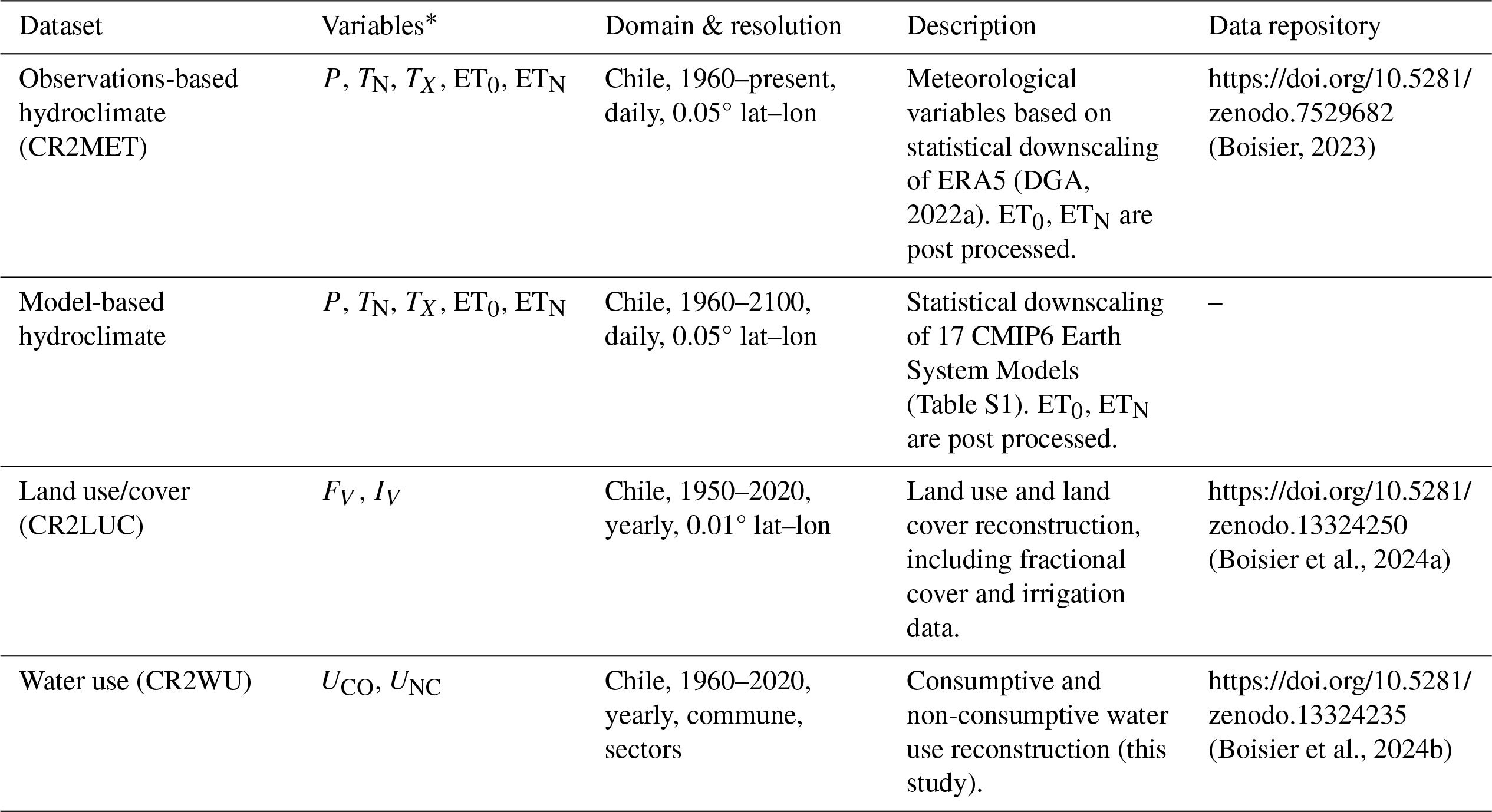
^∗ Precipitation (P), daily minimum (T_N) and maximum (T_X) temperature, potential evaporation (ET₀), naturalized actual evapotranspiration (ET_N), land-cover fraction (F_V), irrigation fraction (I_V), consumptive (U_CO) and non-consumptive (U_NC) water use.

2.1 Historical climate

Daily precipitation and temperature information were obtained from the Center for Climate and Resilience Research Meteorological dataset (CR2MET) version 2.5, available at https://doi.org/10.5281/zenodo.7529682 (Boisier, 2023). The CR2MET product has been developed to fill key data gaps regarding the hydroclimatic mean regime and variability in Chile, and has contributed to scientific and technical knowledge over the past years. In particular, the updated national water balance project led by the National Water Bureau (DGA) has been based on and has boosted the development of CR2MET (see DGA, 2022a, and references therein). CR2MET has been used in a wide range of hydro-climatic research, including the development of the CAMELS-CL catchment dataset for Chile (Alvarez-Garreton et al., 2018), hydrological modeling applications (Baez-Villanueva et al., 2021; Sepúlveda et al., 2022; Araya et al., 2023; Cortés-Salazar et al., 2023), the study of drought dynamics (Alvarez-Garreton et al., 2021; Baez-Villanueva et al., 2024), glacier dynamics (Ruiz Pereira and Veettil, 2019; Amann et al., 2022), water management assessment (Muñoz et al., 2020), and climate change studies (Gateño et al., 2024, Carrasco-Escaff et al., 2024).

The CR2MET dataset includes daily precipitation and diurnal maximum/minimum near-surface temperatures on a regular 0.05° latitude–longitude grid over continental Chile, covering the period from 1960 to the present. These variables are partially built upon a downscaling of the European Centre for Medium-Range Weather Forecasts (ECMWF) ERA5 reanalysis (Hersbach et al., 2020), which uses statistical models calibrated against large, quality-controlled observations of the corresponding variables (P, T_N, T_X). These records gather station data from various national agencies, including DGA, the Weather Service (DMC), the Army Weather Service (SERVIMET-DIRECTEMAR), the Agricultural Research Institute (INIA), and the Foundation for Fruit Development (FDF). This observational dataset is also used in this study for comparison with CR2MET in Sect. 3. The CR2MET statistical models use several atmospheric variables as predictors, selected for the specific predictand (e.g., moisture fluxes are included for P), in addition to land-surface temperature estimates from the Moderate Resolution Imaging Spectroradiometer (MODIS) satellite sensor (Hulley and Hook, 2021) for T_N and T_X. The predictor variables are combined with invariant local topographic features to achieve the target resolution.

A detailed description and validation of CR2MET are provided in DGA (2022a) and references therein. Because CR2MET's statistical models are calibrated using a large observational network in Chile, validation against local meteorological records generally shows low bias and strong covariability in precipitation and temperature compared to other products, particularly in central-southern Chile (DGA, 2018, 2019). Cross-validation analyses further confirm the product's predictive reliability (e.g., DGA, 2018). On a daily time scale, performance tends to decrease in the southern and northern regions of the country, mainly due to weaker covariability between ERA5 and station data in these areas. On monthly or annual time scales, CR2MET generally shows good metrics across the country, making it a useful reference for various applications (e.g., Anderson et al., 2021; Carrasco-Escaff et al., 2023).

The main challenge for spatially distributed products is their ability to extrapolate and provide accurate estimates in data-sparse regions, particularly across the extratropical Andes in the case of Chile. Hydrological simulations, forced by meteorological products such as CR2MET and compared against observed river discharge, offer an objective way to assess their performance in unmonitored areas (e.g., headwater watersheds). This type of validation and the intercomparison with other meteorological datasets consistently demonstrate strong performance (Kling–Gupta Efficiency values typically above 0.6; Baez-Villanueva et al., 2021; DGA, 2022a), with CR2MET outperforming other available products (e.g., Baez-Villanueva et al., 2021). Hydrological balances also allow the identification of systematic biases in precipitation totals within the basins. In this regard, we note that precipitation products – including CR2MET – likely underestimate precipitation in Chile's wettest watersheds, particularly in the southern Andes and western Patagonia (Alvarez-Garreton et al., 2018).

For this study, potential evapotranspiration (ET₀) is derived as a post-processed CR2MET variable over the same spatiotemporal domain. Due to data availability from CR2MET and downscaled climate models (Sect. 2.2), the method is based on the temperature-dependent Hargreaves-Samani (HS) formula (Hargreaves and Samani, 1985), which is then corrected using two criteria: (1) accounting for systematic biases between the HS estimate and the more precise, multivariate Penman-Monteith (PM) formula (e.g., Allen et al., 1998), and (2) accounting for mean biases in wind conditions. For a given grid cell (x) and day (t), the adjusted ET₀ is computed as follows:

$$\begin{array}{}\text{(1)}& {\text{ET}}_{\mathrm{0}}(x,t)=A(x,t_{\mathrm{0}}){\text{ET}}_{\text{0,HS}}(x,t)+B(x,t_{\mathrm{0}})\end{array}$$

where ET_0,HS is the HS estimate as described by Samani (2000). The formula is used with T_N and T_X from CR2MET and daily mean temperature calculated as the average of these two variables. Coefficient A is computed as the climatological mean (1981–2015) PM to HS-based ET₀ ratio (ET${}_{\mathrm{0},\mathrm{PM}}/{\text{ET}}_{\mathrm{0},\mathrm{HS}}$), using a consistent set of atmospheric variables; in this case, the ERA5 reanalysis. The ERA5 HS-based ET₀ is calculated in the same manner as that derived with CR2MET, but with the corresponding $T_{\mathrm{N}}/T_X$ data. The ERA5 PM-based ET₀ corresponds to the Singer et al. (2021) dataset. It should be noted that the use of factor A assumes that PM/HS corrections, valid – by construction – for ERA5 data, also apply to CR2MET data, likely introducing some inaccuracies. Coefficient B addresses a wind bias correction, based on the comparison of near-surface wind speed data from ERA5 (consistent with the PM to HS correction applied with coefficient A) and a source with more spatial detail than ERA5. In this case, we used 1 km simulations (aggregated to the 0.05° CR2MET grid) conducted in Chile with the Weather Research and Forecasting (WRF) model for the Wind Energy Explorer (https://eolico.minenergia.cl/, last access: 1 October 2023; see Muñoz et al., 2018). This correction is based on simplified aerodynamic expressions typically used to estimate open water evaporation, which scales with the air vapor pressure deficit (VPD) and a coefficient depending on wind speed (the so-called wind functions, e.g., Penman, 1948). We used the wind function parameterization described by McJannet et al. (2012) and VPD from ERA5 to compute B as 0.167 (U_WRF−U_ERA5) VPD. Here, U_WRF and U_ERA5 correspond to the climatological mean 2 m wind speed from the WRF and ERA5, respectively. Both coefficients A and B are spatially distributed and computed separately for each month of the year, and then interpolated to Julian days (t₀ in Eq. 1).

2.2 Climate model downscaling

To assess the impacts of anthropogenic climate change on water availability and water stress, we used an ensemble of Earth System Model (ESM) simulations from the sixth phase of the Coupled Model Intercomparison Project (CMIP6). The ESM data were bias-corrected for the period 1960–2100 to accurately represent Chile's hydroclimate and properly contrast with observation-based data.

The applied bias correction method is based on the Quantile Delta Mapping (QDM) approach as described by Cannon et al. (2015), using CR2MET as the reference dataset. Unlike conventional quantile mapping, the QDM method adjusts the frequency distribution of a given variable to match a reference (typically an observational record or an observations-based time series) while preserving the modeled changes in the variable's quantiles over time. The method was applied on a daily time scale to precipitation outputs from 17 ESMs and to a subset of 11 ESMs for daily extreme temperatures, according to data availability at the time of the analysis (Table S1 in the Supplement). Simulations include historical runs and future projections forced by two socio-economic scenarios: Shared Socioeconomic Pathways (SSPs) 1 and 3 (Global Sustainability and Regional Rivalry), respectively paired with carbon emissions pathways leading to radiative forcing levels of 2.6 and 7.0 W m⁻² by 2100 (Eyring et al., 2016; O'Neill et al., 2016). These two scenarios, SSP1-2.6 and SSP3-7.0, represent high and medium-to-low climate change mitigation efforts during the current century, with associated climate simulations available for a large ensemble of models.

The QDM computations were applied additively for absolute changes in T_N and T_X, and multiplicatively for relative changes in P. The parametric density distributions Generalized Extreme Value and Exponential were used to fit the empirical frequency distributions of $T_{\mathrm{N}}/T_X$ and P, respectively. To ensure accurate seasonal representation, the method was applied separately for each month of the year. Additionally, post-corrections were made to address any evident physical inconsistencies; for example, if T_X was found to be less than T_N, both variables were adjusted to their average value.

The downscaled temperature data is then used to estimate ET₀ in models using the same HS-based approach described in Sect. 2.2. Precipitation and ET₀ data both from in CR2MET and ESMs are used to estimate a naturalized evapotranspiration, as described in the next section.

2.3 Hydrological balance and water availability

Water availability (A) is considered here as a naturalized runoff, computed as the remaining flow from precipitation (P) and evapotranspiration (ET), without considering local disturbances (Eq. 2). This definition aligns with Renewable Freshwater Resources (RFWR), according to several references (e.g., Vörösmarty et al., 2000; Alcamo et al., 2003; Oki and Kanae, 2006; Wada et al., 2011; Kuzma et al., 2023). Renewable water availability includes natural groundwater recharge and thus renewable groundwater resources, however, there is a non-renewable groundwater component that, by definition, is not included in A. It should be noted that groundwater can supply water beyond the renewable recharge, which leads to sustained storage depletion, as reported by recent studies in central Chile (Jódar et al., 2023; Alvarez-Garreton et al., 2024; Taucare et al., 2024).

Thus, the surface water budget in a hydrological unit is represented as follows:

$$\begin{array}{}\text{(2)}& A=P-{\text{ET}}_{\mathrm{N}}=R_{\mathrm{N}}\end{array}$$

where ET_N and R_N stand for naturalized evapotranspiration and runoff. For simplicity, since A is assessed on a yearly to multi-year basis, changes in water storage are omitted in Eq. (2), but soil water content dynamic is accounted for in smaller-scale ET computation (Appendix A). The disturbed water budget is represented as:

$$\begin{array}{}\text{(3)}& A-\mathrm{\Delta }{\text{ET}}_{\mathrm{LU}}-U_{\sim \mathrm{LU}}=R_{\mathrm{N}}-\mathrm{\Delta }R\end{array}$$

where ΔET_LU and U_∼LU indicate, respectively, modified ET due to land use/land cover changes (defined as positive for a perturbation increasing ET) and losses by other means (consumptive water use from other activities), both of which will induce a change in runoff (ΔR).

Fluxes of ET were computed over continental Chile with the same spatiotemporal resolution as CR2MET, using a simplified “bucket” ET scheme described in Appendix A. This model runs on daily time steps, forced by P and ET₀ from CR2MET or from CR2MET-based downscaled climate model data to maintain a consistency in observed and modeled data. The ET scheme also depends on soil and land cover parameters, and accounts for well-watered surfaces to represent water bodies and irrigated areas, allowing the estimation of both ET_N and ΔET_LU.

For ET_N, historical simulations were performed using the CR2MET forcing between 1960 and 2020, with irrigation turned off and prescribing a static land-cover map of 1950, according to the CR2LUC product (Sect. 2.4). Thus, more precisely, ET_N represents a climate-dependent ET flux under past land-cover conditions, without irrigation or temporal land use changes. Subsequently, annual time series of A for each basin were computed as the difference between catchment-scale annual P and ET_N (Eq. 2). Projections of water availability following the SSP1-2.6 and SSP3-7.0 scenarios were derived in the same way but using the downscaled ESM data as climate forcing. As part of the water use reconstruction workflow, the computation of ΔET_LU is described in Sect. 2.5.

2.4 Land cover reconstruction

Long-term land-use dynamic is a key factor to consider when estimating changes in water use over time and for many other applications. The CR2LUC product was developed for this end, describing land use and land cover changes in Chile since 1950. As it encompasses a pre-satellite period, this reconstruction was developed using a different approach from typical land use/cover estimates available for more recent decades.

Although satellite data are used for fine spatial distribution guidance, the reconstruction is based on national bookkeeping of land use activities in Chile, particularly agricultural censuses conducted since 1930. The methodological challenge in developing CR2LUC lies in the homogenization and coherent integration of information from different sources, as well as the data preprocessing of each source (e.g., some historical documents required data digitization/tabulation). The assessed set of inventoried data includes the Agricultural and Livestock Censuses carried out by the National Institute of Statistics (INE) for the years 1955, 1965, 1976, 1997 and 2007 (see references in the Supplement), the Continuous Statistics of annual crops from the Office of Agricultural Studies and Policies since 1979 (ODEPA, 2023b), the Fruit Cadastres maintained by the Natural Resources Information Centre and ODEPA since 1998 (CIREN-ODEPA, 2023), the Viticultural Cadastres from the Agricultural and Livestock Service (SAG) since 1997 (ODEPA, 2023a), and the Vegetation Cadastres from the National Forestry Corporation, maintained since 1993 (CONAF, 2023).

The first stage of the CR2LUC workflow involves computing continuous time series describing annual quantities, primarily the fractional land area occupied by a given land cover class, for every commune in the country between 1950 and 2020, ensuring alignment with data provided by agricultural censuses in specific years. To achieve this, solutions were developed to transform census data provided for different territorial units over time into a unified classification (current communes). In most cases, this was done by extrapolating proportional relationships in given variables between nested or related units (e.g., current communes vs. old provinces in Chile, or communes created from a larger, former one). Interpolation methods were used to fill in the time series, ranging from simple statistical criteria (e.g., linear interpolation) to guidance based on other sources, depending on data availability in different periods (e.g., cadastres provided by ODEPA).

A finer spatial disaggregation (gridding) of the communal-level values was driven by satellite information and some inventories available at high resolutions in recent years (e.g., fruit orchard cadastres), while ensuring consistency with aggregations provided at larger (territorial) unit scales. Cropland and urban areas were constrained by the corresponding classes in Landsat-based land cover datasets developed for Chile by Zhao et al. (2016) and globally by Chen et al. (2015), with the latter including three scenes for 2000, 2010, and 2020. Vegetation cadastres of CONAF were the main input used to distribute natural vegetation classes and tree plantations, as well as to define a potential vegetation for past periods. Other inputs include fine national inventories (polygons) of water bodies, wetlands, saltpans (MMA, 2020), and glaciers (DGA, 2022b).

As result, CR2LUC provides fractional land cover data on a 1 km latitude-longitude grid for continental Chile, with annual data from 1950 to 2020. It also includes information on irrigation (grid fraction and type) and yields for specific crops. Organized into three levels of aggregation, the dataset includes a total of 48 classes of relevance in Chile (Table S2), encompassing various agricultural types (25), natural forests (5), planted trees (3), shrubland (3), grasslands (3), natural and artificial water bodies (5), salt pans, glaciers, built-up areas and bare soil. Hence, in addition to the temporal coverage, the dataset is characterized by a detailed classification. Version 1.0 of CR2LUC, used in this study, is available on https://doi.org/10.5281/zenodo.13324250 (Boisier et al., 2024a).

2.5 Water uses reconstruction

The CR2WU product was developed to assess historical water demand in Chile. This dataset provides water use estimates as volumetric fluxes (U) from various sectors for each commune in continental Chile, with annual resolution from 1960 to 2020. The dataset includes consumptive uses for all sectors considered, as well as non-consumptive uses for two sectors with major return flows: hydroelectric generation and irrigated agriculture. The computation involves two distinct methodologies: one for sectors encompassing land use, land-use change, and forestry (LULUCF) and another for other water-consuming sectors, including drinking water, energy, mining, manufacturing industry, livestock, with corresponding subcategories (Table S3).

For LULUCF sectors, water uses were derived using the ET scheme introduced in Sect. 2.3 (further described in Appendix A), as the difference between alternative historical ET scenarios. One scenario represents the actual ET, following the historical land use/cover, irrigation, and climate conditions (ET_FULL), and another – control – scenario represents ET with no land use/cover changes, corresponding to ET_N (Sect. 2.3). A third simulation was performed in the same way as ET_FULL but without irrigation (ET_NI), allowing the estimation of the ET change component driven by rainfed agriculture and forestry (the “green” water use), as well as by modifications in water bodies. We note that the latter includes all types of artificial reservoirs, so consumptive water use due to evaporation losses from hydroelectric power dams is included within LULUCF, rather than under the energy sector. Hence, the consumptive total water use from LULUCF (U_CO,LU) and the non-irrigated component ($U_{\mathrm{CO},\mathrm{LU},\mathrm{NI}}$) were computed as:

$$\begin{array}{}\text{(4)}& {\displaystyle }{U}_{\mathrm{CO},\mathrm{LU}}\left(\mathrm{yr}\right)={\mathrm{ET}}_{\mathrm{FULL}}\left(\mathrm{yr}\right)-{\text{ET}}_{\mathrm{N}}\left(\mathrm{yr}\right)\text{(5)}& {\displaystyle }{U}_{\mathrm{CO},\mathrm{LU},\mathrm{NI}}\left(\mathrm{yr}\right)={\text{ET}}_{\mathrm{NI}}\left(\mathrm{yr}\right)-{\text{ET}}_{\mathrm{N}}\left(\mathrm{yr}\right)\end{array}$$

Irrigation fractions from CR2LUC are used to prescribe unlimited soil moisture in the corresponding grid cells and agricultural classes, while the irrigation type is used to estimate the water supply typically needed for irrigation practices, a portion of which returns to the system as infiltration (a non-consumptive use). Irrigation efficiency (e_IR), defined as the ratio between U_CO,LU and the total irrigation volume, was set to 0.5, 0.6, and 0.75 for the three types of irrigation included in CR2LUC: traditional (e.g., furrow), mechanized (sprinkler), and localized, according to Brouwer et al. (1989). In this way, the non-consumptive water use component of agriculture (U_NC,LU) was derived as:

$$\begin{array}{}\text{(6)}& U_{\mathrm{NC},\mathrm{LU}}\left(\mathrm{yr}\right)=\left(e_{\mathrm{IR}}^{-\mathrm{1}}-\mathrm{1}\right)U_{\mathrm{CO},\mathrm{LU}}\left(\mathrm{yr}\right)\end{array}$$

Sectors other than LULUCF were grouped into drinking water, livestock, energy, mining, and manufacturing industries, each with various subsectors (Sect. 4 and Table S3). Water use for these sectors was estimated using methodologies from previous studies commissioned by DGA (e.g., DGA, 2017). These studies quantified water consumption for a specific year based on sector-specific forcing data (e.g., mineral mass production for the mining sector) and consumption rates specific to each class (e.g., water usage per tonne of copper concentrates). Having established the consumption rate values specific to each sector or process, the major challenge for historical water use estimation was reconstructing the evolution of sector-specific drivers. To obtain continuous time series from the mid 20th century to the present, we followed a methodology similar to that described for the CR2LUC dataset. Various documents and national inventories were homogenized to get continuous spatio-temporal series of the forcing data for each sector (F_S). This information was then combined with water consumption rates (K_S) to estimate the volumetric water use as follows:

$$\begin{array}{}\text{(7)}& U_{\mathrm{S}}(x,\mathrm{yr})=K_{\mathrm{S}}\cdot F_{\mathrm{S}}(x,\mathrm{yr})\end{array}$$

In DGA (2017), drinking water was treated separately, with total withdrawals estimated alongside a return flow component, calculated based on sanitary data. However, in Chile, data on wastewater flows and discharge locations – necessary for reconstructing historical return flows – are not publicly available. Due to this limitation, this component was not estimated in our study, and the WSI calculation includes total withdrawals for this sector, whereas for other sectors only the consumptive component is considered (Sect. 2.6). For coastal locations in Chile, this approach is appropriate, as most wastewater treatment plants discharge directly into the sea via submarine outfalls (Gómez et al., 2025), making drinking water withdrawals effectively fully consumptive at the basin scale. In other cases, where wastewater is discharged upstream of the basin outlet, water quality considerations provide additional justification for this choice. Indeed, the Chilean law prohibits the reuse of treated greywater in key sectors such as potable water supply, irrigation of fruits and vegetables that grow at ground level, food production, healthcare facilities, and aquaculture (MOP, 2023).

Table S3 in the Supplement provides a full list of sectors, their consumption factors, and the forcing variables and sources. While estimates for LULUCF are computed on a regular grid, water use data is aggregated and reported at the communal scale, with annual estimates from 1960 to 2020. CR2WU data are available at https://doi.org/10.5281/zenodo.13324235 (Boisier et al., 2024b).

2.6 Computation of water stress index and its drivers of change

The WSI, here defined as a water demand-to-availability ratio (Falkenmark and Lundqvist, 1998), depends on how both components are quantified, potentially leading to different outcomes (Liu et al., 2017a). Most previous studies using this index rely on water use estimates based on gross demand (as a proxy for total withdrawals, e.g., Vörösmarty et al., 2000; Oki and Kanae, 2006; Kuzma et al., 2023), while others consider net demand (equivalent to consumptive use, e.g., Wada et al., 2011), or assess both measures (e.g., Munia et al., 2016). Using total withdrawals in basins with large return flows – such as in Chile, where many watersheds are modified for hydroelectric power generation – results in very high WSI values that do not necessarily reflect actual water stress. For this reason, and to preserve a water balance rationale, only consumptive uses are considered in the WSI calculation in this study. Accordingly, the WSI is defined as the ratio $U_{\mathrm{CO}}/A$, where U_CO and A represent total consumptive water use and near-natural water availability, respectively, as described in previous sections. The WSI is computed at multi-annual timescales for hydrological units, specifically over the major watersheds defined by the DGA in the National Inventory of Watersheds (BNA).

As explained in Sect. 2.5, we considered total drinking water requirements as consumptive use, acknowledging that in some watersheds, return flows from water treatment can be potentially reused. It is important to note that, in contrast to previous WSI estimates (e.g., Vörösmarty et al., 2000; Oki and Kanae, 2006), and in line with more recent recommendations (e.g., Rockström et al., 2010; Hoekstra et al., 2011; Liu et al., 2022), we include green water use. That is, consumptive water use from forestry and rainfed agriculture is incorporated, estimated as the differential ET loss between land use scenarios (see Sect. 2.5).

Regarding water stress classification based on the WSI, many studies have adopted a reference threshold of 40 %, above which a basin is considered water-stressed (e.g., Falkenmark and Lundqvist, 1998; Vörösmarty et al., 2000; Alcamo et al., 2003; Oki and Kanae, 2006; Falkenmark et al., 2007; Wada et al., 2011; Munia et al., 2016; Kuzma et al., 2023). WSI levels have been linked to the concept of water crowding, with values between 40 % and 70 % typically indicating high water stress, and values above 70 % representing extreme stress – when water use begins to affect volumes that should be reserved for environmental flows (see Falkenmark et al., 2007, and references therein). From an ecological flow perspective, Pastor et al. (2014) reviewed several methods for estimating environmental flow requirements. On average, these methods recommend preserving between 34 % and 56 % of the mean annual flow, which corresponds to a maximum WSI of approximately 44 % to 66 %. Similar ecological flow requirements have been estimated for watersheds in Chile using different methodologies (Alvarez-Garreton et al., 2023a). These findings support the idea that WSI levels above 40 % may pose risks to fluvial ecosystems and reinforce the 70 % threshold for extreme stress, as ecological flow protection is generally not ensured beyond this point.

Given the simplicity of the WSI, it allows for a straightforward estimation of the relative impact on water stress levels resulting from variations in both water availability (climate-driven supply) and water use (demand), as presented in Sect. 5. The evolution over time driven by changes in water availability (ΔWSI|_A) and use (ΔWSI|_U) are estimated by decomposing the WSI ratio into its partial derivatives, leading to:

$$\begin{array}{}\text{(8)}& {\displaystyle }\mathrm{\Delta }\text{WSI}{\mathrm{|}}_A=-C\stackrel{\mathrm{‾}}{\mathrm{WSI}}{\displaystyle \frac{\mathrm{\Delta }A}{\stackrel{\mathrm{‾}}{A}}}\text{(9)}& {\displaystyle }\mathrm{\Delta }\text{WSI}{\mathrm{|}}_U=C\stackrel{\mathrm{‾}}{\text{WSI}}{\displaystyle \frac{\mathrm{\Delta }U}{\stackrel{\mathrm{‾}}{U}}}\end{array}$$

Terms with Δ denote the difference of the corresponding variable between two periods of interest, and the overbar indicates the average over the two periods. Since the calculation is not performed on an infinitesimal scale, the sum of the partial derivative terms does not precisely match the total change in WSI. To address this, both terms are adjusted proportionally (constant C in Eqs. 8 and 9) so that their sum equals the absolute change in WSI between the evaluated periods.

3 Historical and future changes in water availability (1960–2100)

Due to the latitudinal distribution and complex topography of Chile's continental territory, there is a large contrast in precipitation regimes from the hyperarid Atacama Desert (with virtually no precipitation) to extremely rainy areas in the southern Andes and Patagonia (with annual accumulations exceeding 3 m, Fig. 1).

As in other regions of the globe, potential evapotranspiration (ET₀) in Chile follows an inverse pattern to precipitation, with maximum values (above 2000 mm yr⁻¹) in the north of the country due to the high insolation and atmospheric water demand in the desert (Fig. 1b). The surface water limitation north of ∼30° S and the ET₀ threshold south of ∼40° S (below 1000 mm yr⁻¹) define the distribution of actual ET. The region in between, central Chile, features a mixed hydroclimate resulting from a sharp transition between water-limited regimes in the north and energy-limited areas in the south. This region, home to most of the country's population and economic activities, is also characterized by Mediterranean-like precipitation seasonality with dry summers and high inter-annual variability (Boisier et al., 2018; Aceituno et al., 2021).

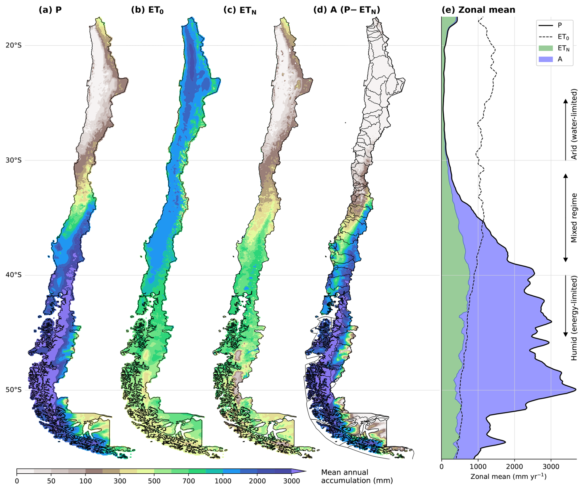
Figure 1 Long-term (1990–2020) mean annual precipitation (a), potential evapotranspiration (b), near-natural evapotranspiration (c), and water availability (d) in continental Chile. Panel (e) shows the zonal average of each water flux and the balance between P, ET_N and A. Thin polygons in panel (d) indicate the country's major watersheds (BNA).

On average across continental Chile, the mean annual rates of P and ET_N are estimated at 1200 and 430 mm, respectively, which leads to a surface water availability of approximately 770 mm yr⁻¹ (equivalent to a volumetric flux of 680 km³ yr⁻¹). A similar value is estimated in DGA (2022a), which also uses the CR2MET dataset, while a higher value – approximately 1050 mm yr⁻¹ – is reported by FAO (2021) as Chile's renewable water resources. Beyond these differences, Chile's average freshwater availability remains high compared to other countries; the global mean over continental areas is close to 300 mm yr⁻¹ (Oki and Kanae, 2006). However, conditions vary greatly across the country, as the gap between P and ET_N defines a pronounced north-to-south gradient of water availability (see panels d and e in Fig. 1). Specifically, the administrative regions of Los Lagos, Aysén, and Magallanes (south of 40° S) together account for more than 75 % of the total available water volume in the country, whereas the regions from Valparaíso (∼32° S) northward add up to less than 1 % of the total, underscoring stark regional disparities and contrasting water security challenges in Chile.

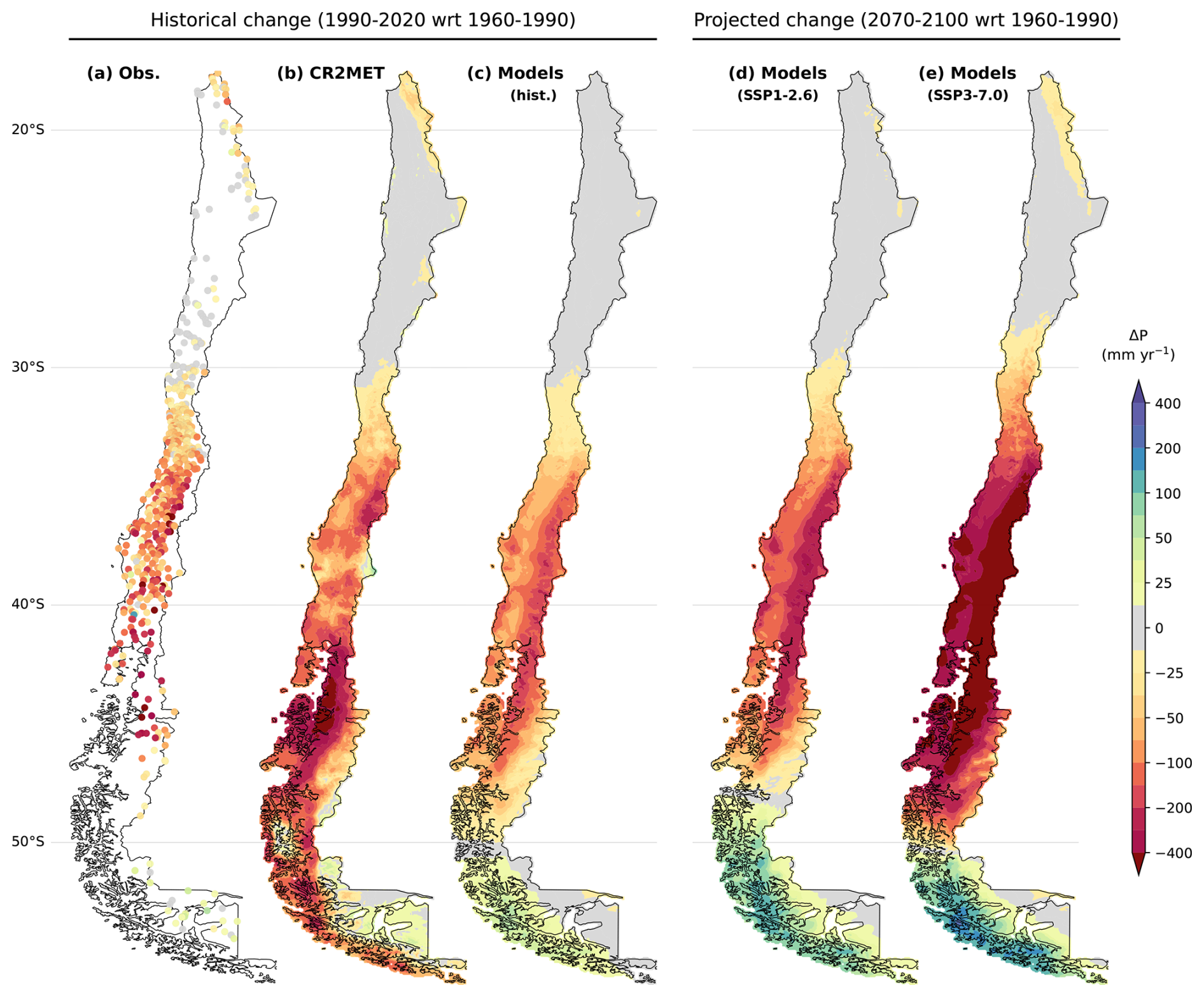
Figure 2 Changes in mean annual precipitation in Chile between the periods 1960–1990 and 1990–2020 (a–c), and projected towards the end of the 21st century (2070–2100) under global scenarios SSP1-RCP2.6 (d) and SSP3-RCP7.0 (e). Historical changes are based on local observations (a), the CR2MET dataset (b), and CMIP6 model simulations (historical scenario and SSP3 for 2015–2020). The three modeled changes (c–e) are based on downscaled simulations from 17 CMIP6 ESMs (showing the multi-model mean).

Besides geographical differences, Chile's hydroclimate exhibits an important temporal variability. Over the long term, local precipitation records show a clear downward trend, as shown by the changes in mean annual precipitation between the periods 1960–1990 and 1990–2020 across much of the country (Fig. 2a). The spatially distributed CR2MET dataset shows a precipitation decline consistent with observations (Fig. 2b), a match that matters given the subsequent use of this dataset for basin-scale assessments.

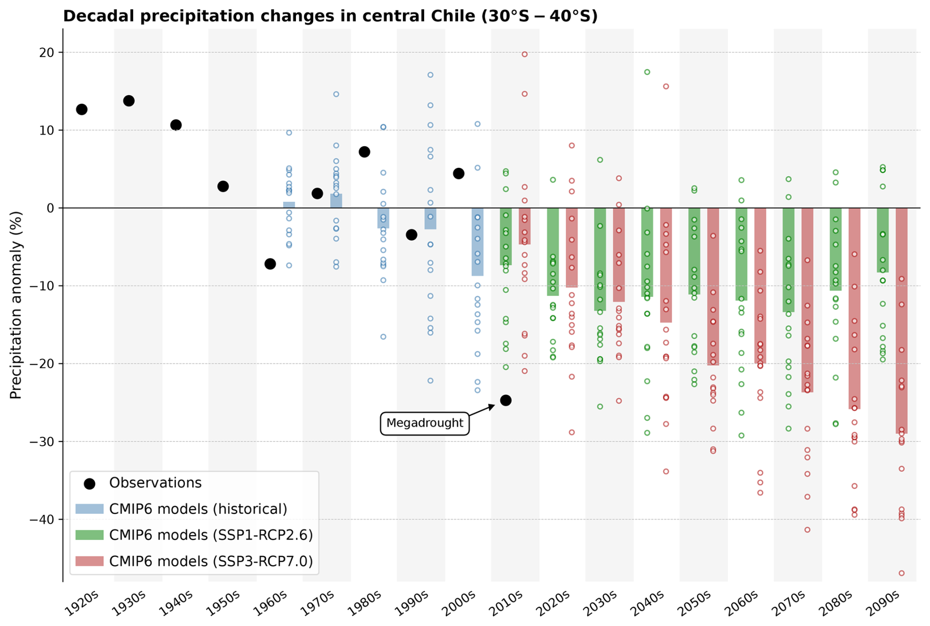
Figure 3 Precipitation changes in central Chile (30–40° S). Decadal mean precipitation anomalies relative to the 1960–1990 period, based on observations (black circles) and downscaled simulations from 17 ESMs (circles and bars show single and multi-model mean values). Model data based on CMIP6 simulations under the historical (blue), SSP1-RCP2.6 (green), and SSP3-RCP7.0 (red) scenarios.

Studies addressing the driving mechanisms of the recent megadrought and long-term climate trends in Chile indicate that changes in precipitation result from natural climate variability and anthropogenic climate change, with the latter being more prominent in the long-term (Boisier et al., 2016, 2018; Garreaud et al., 2017, 2019; Damiani et al., 2020; Villamayor et al., 2021). These conclusions are based on the contrast between observations and simulations with global climate models, which systematically simulate a decrease in precipitation over the South Pacific in response to changes in greenhouse gas and stratospheric ozone concentrations (IPCC, 2022). This decrease precisely affects the country's regions where trends towards a drier climate are observed. The downscaled simulations from the CMIP6 ensemble assessed here are broadly consistent with observation-based changes, although slightly lower in magnitude (Fig. 2). This difference could be related to an additional drying driven by natural multidecadal changes and the recent megadrought in central Chile (Fig. 3), and/or to a higher actual regional sensitivity to anthropogenic forcing compared to the model average (Boisier et al., 2018).

The drying tendency overlaps with short-term variability, as seen in decadal precipitation anomalies in central Chile (Fig. 3). On this time scale, the magnitude of the recent megadrought stands out and underscores the importance of considering low-frequency natural climate variability in water governance and planning, as well as its role in climate projection uncertainty.

Following Hawkins and Sutton (2009), the projected precipitation changes shown in Fig. 3 are highly variable and depend on three main sources of uncertainty: (1) the overlap of the climate change signal with phases of natural variability that can last for decades, (2) the intensity of the global and regional climate change signal, with differences among climate models, and (3) the global socioeconomic scenario considered. Considering these factors, in an optimistic case, a decrease in precipitation of less than 10 % can be expected in central Chile by the end of the 21st century. This projection is based on a global scenario with high mitigation of greenhouse gas emissions (SSP1-RCP2.6, O'Neill et al., 2016) and models with low regional climate sensitivity to anthropogenic forcing. In a pessimistic case, the deficit may exceed 30 %, resulting in conditions like the 2010s' megadrought but permanently. This regime represents an average condition, and even drier decades (deficits above 40 %) can be anticipated in the region due to the superposition of natural droughts with climate change. This scenario is projected with medium to high global greenhouse gas emissions (SSP3-RCP7.0) and models with high climate sensitivity.

4 Current conditions and historical changes in water uses (1960–2020)

Water withdrawals for both human consumption and productive purposes have diverse impacts on water balances (Wada et al., 2011). These impacts largely depend on whether the withdrawn water is returned to the basin, termed non-consumptive use (e.g., in hydroelectric generation), or not returned, known as consumptive use (e.g., water evaporated in industrial and land use activities).

In Chile, most water-intensive activities are concentrated in the country's central and northern regions (Fig. 4). Considering both consumptive and non-consumptive uses, the total water use is estimated at around 100 km³ yr⁻¹ in the last decade (2010–2020). This value is higher than those reported by other independent estimates (DGA, 2017; Fundación Chile, 2018; FAO, 2021; Appendix B). Although the comparison among available estimates is not straightforward – due to differences in methodologies, sectors, or periods considered – there remains a considerable degree of uncertainty in some key sectoral water use estimates, particularly within the LULUCF sector (Table B1). Reducing this uncertainty is important for the effective design and implementation of public policies.

Compared to other countries, total water use in Chile is high, primarily due to the presence of several hydroelectric power generation plants in mountainous basins of the central-southern regions. This process involves using a large volume of water, but which is almost entirely returned to the system, except for losses from reservoir evaporation (as noted in Sect. 2.5, this consumptive component is accounted for within the LULUCF sector rather than in Energy). Thus, hydroelectric water use primarily alters the flow dynamics of the intervened river but does not substantially affect the long-term water balance of the basin at its discharge into the sea.

Consumptive water use is primarily attributed to the LULUCF sector, whose main activities are concentrated in central Chile (Fig. 4). With a total flow estimated at 11.5 km³ yr⁻¹ (∼365 m³ s⁻¹), this sector accounts for nearly three-quarters of the country's consumptive water use. Specifically, irrigated agriculture consumes a large volume of water (∼9 km³ yr⁻¹ or 285 m³ s⁻¹) due to high rates of crop evapotranspiration, often located in water-limited areas with elevated ET₀. Non-irrigated LULUCF activities also represent a significant share (nearly 15 %) of national consumptive water use – a green water footprint –, and constitute the principal water use sector in several communes of central Chile (Fig. 4e). The non-irrigated LULUCF water use is mainly associated with forestry plantations, and to a lesser extent with rainfed agriculture and evaporation from artificial water bodies. We note that this estimate is subject to considerable uncertainty, with notably higher value reported previously (Table B1).

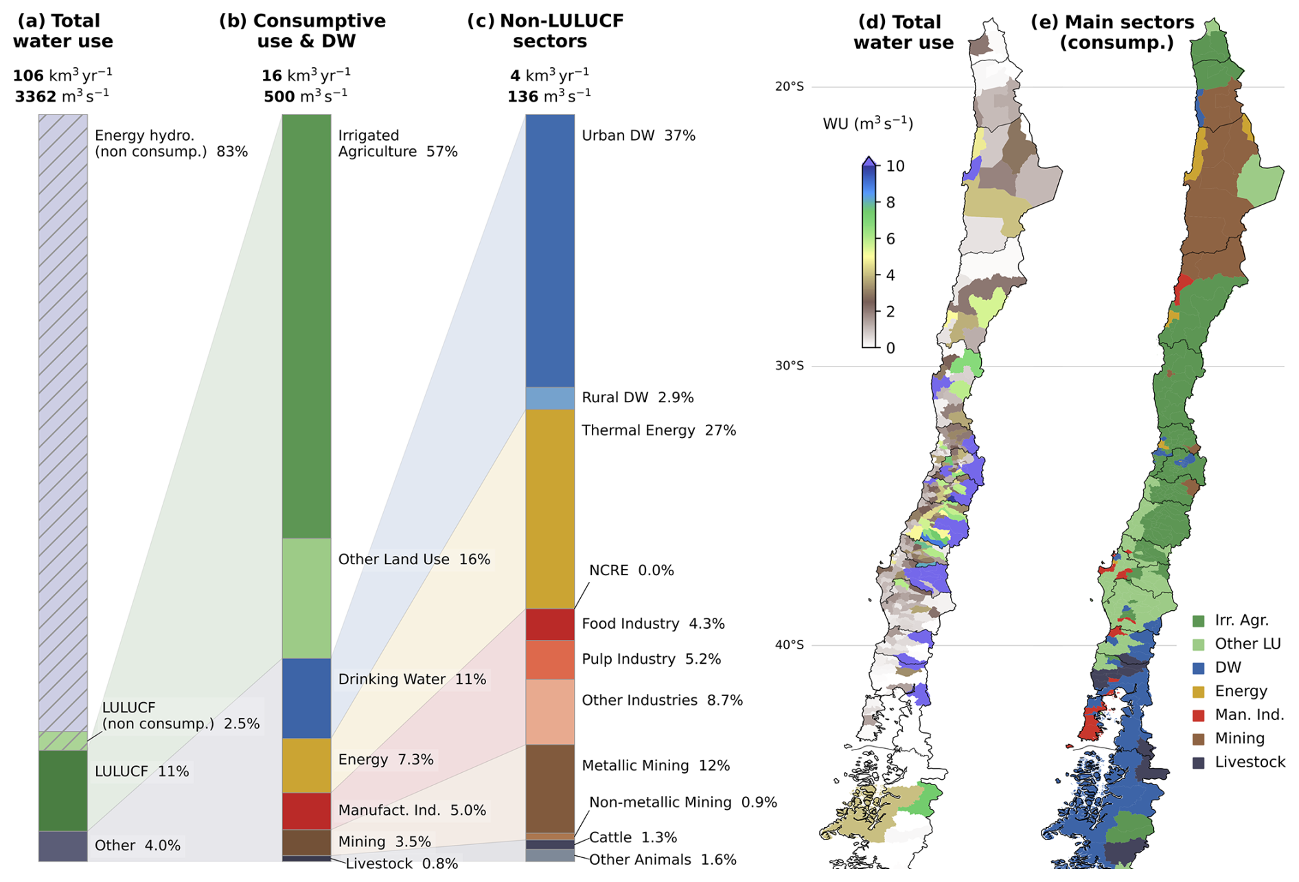
Figure 4 Near-present water use in Chile (2010–2020 average). Bars (a–c) indicate the total national water use and sectoral contributions, including the details of drinking water withdrawals (DW) and consumptive water use sectors (b), and the non-LULUCF sub-sectors (c). Maps show the distribution of water use by commune across the central and northern regions of the country (d), and the dominant sectors driving communal consumptive water use (e).

Agriculture also includes a non-consumptive water use component, as a portion of irrigation water returns to the system through infiltration and percolation. For the near-present period, the return flow is estimated at about 2.7 km³ yr⁻¹, corresponding to 23 % of the total water withdrawn for irrigated agriculture (Fig. 4a and Table B1). This return flow, as a proportion of total irrigation, reflects irrigation efficiency, which tends to decrease as more advanced technologies and improved management practices are adopted.

According to our methodology, certain land use activities may result in negative water use – that is, landscape transformations that reduce ET compared to ET_N. This response is obtained in urban areas and some pasture lands in southern Chile, though its magnitude is very low at the national level.

Water supply systems, from extraction to treatment and wastewater return, constitute a partially consumptive water use sector totalling around 55 m³ s⁻¹ in Chile. This use is mainly associated with supply in urban areas, of which 30 m³ s⁻¹ (equivalent to 145 L per person per day) corresponds to domestic consumption. Hence, on average, the provision of drinking water for human consumption in Chile meets the minimum standard of 100 L per person per day, although there are large contrasts within the country, including areas with serious supply problems (Muñoz et al., 2020; Meza et al., 2014; Duran-Llacer et al., 2020; Alvarez-Garreton et al., 2023b).

Consumptive water uses of the energy sector (mostly thermoelectric power plants), mining, livestock, and manufacturing industry play a secondary role in the national total but may be large – and often dominant – at the local or watershed scale, particularly in the arid northern areas (see Fig. 4e).

Alongside population growth and socioeconomic development, water use in Chile increased substantially over the past six decades (Fig. 5). The LULUCF sector was the main driver, with water use rising from about 240 to 365 m³ s⁻¹ (53 %), explaining most of the growth in consumptive use since the 1960s. In particular, water use in irrigated agriculture has risen by approximately 20 % due to increased production of annual crops and strong development in the fruit orchard industry, the latter with greater relevance within the central-north valleys, featuring high insolation and drier conditions.

This increase in water use in agriculture has occurred despite a widespread transition from gravitational to sprinkler and drip irrigation systems, which has enhanced irrigation efficiency over the last four decades. Indeed, among the various sectors, the non-consumptive water use component of irrigated agriculture has been the only one featuring a downward trend (not shown). Part of these changes can be explained by the irrigation efficiency paradox, which refers to cases where improvements in irrigation efficiency reduce non-consumptive water use but do not result in actual water savings at the basin scale. Instead, increased efficiency enables the irrigation of a larger cropping area or the cultivation of more water-intensive crops, ultimately leading to higher consumptive water use – especially when total water extractions are not regulated (Grafton et al., 2018).

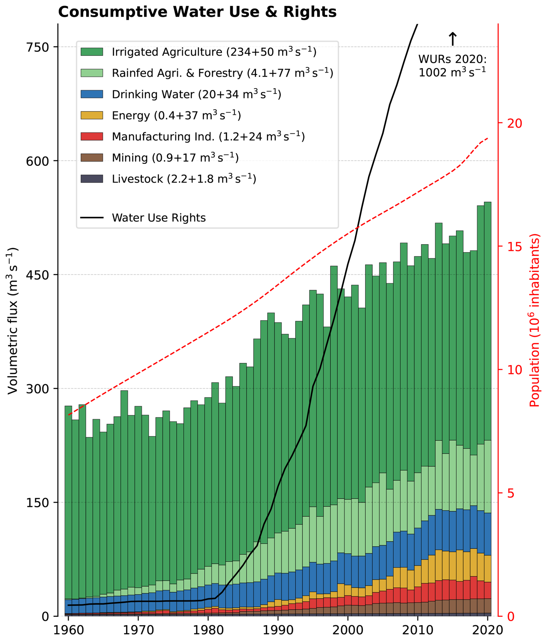
Figure 5 Historical evolution (annual means) of consumptive water use and allocated rights (WURs, black curve) in Chile. The values in the legend indicate the average water use during the 1960s and the increase towards the 2010s for each sector. Dashed curve (red axis) shows the country's population (source: World Population Prospects, UN, 2024).

The forestry industry, which developed primarily between the 1970s and 2000s, has also largely contributed to the increase in water use (about 80 m³ s⁻¹; Fig. 5) and to greater pressure on water resources in watersheds with intensive Pinus radiata and Eucalyptus plantations, particularly along the coastal range of central Chile. This finding aligns with previous assessments of water consumption by tree plantations in Chile (e.g., Alvarez-Garreton et al., 2019; Galleguillos et al., 2021; Balocchi et al., 2023) and in other regions worldwide under similar conditions (e.g., Farley et al., 2005; Beets and Oliver, 2007).

Due to changes in the LULUCF sector, the growth in productive sectors, and the population increase, the total consumptive water demand has doubled over the study period (Fig. 5). Additionally, during the second half of the 20th century, non-consumptive uses grew more than fourfold due to the major implementation of hydroelectric power plants (not shown). In the 21st century, the installed energy capacity and generation continued to grow, primarily through thermoelectric plants, which have an important consumptive water use (Fig. 5), and more recently, through solar and wind power plants, which have very low water consumption.

The water use estimates presented in this section are based on actual socioeconomic activities in Chile (Sect. 2.5), regardless of whether these activities have a WUR granted by the State. The regulation regarding the access to freshwater sources for consumptive or non-consumptive uses through WURs has been systematic since the introduction of the Water Code in 1981, which is still in force in the country (Congreso Nacional de Chile, 2022). This regulation has formalized customary rights and granted new ones, leading to the steeply increasing curve of the total allocated consumptive flow in Chile since the early 1980s (black curve in Fig. 5). As expected, the national water use estimated here for the present time is below the exploitable volume according to the allocated consumptive WURs, which totals about 1000 m³ s⁻¹ across the country. However, there are exceptions in some basins where uses are supplemented by desalinated sea water, which is not recorded under WURs, as they only consider terrestrial freshwater sources. An example is the coastal basin of Quebrada Caracoles in the Antofagasta region (∼23° S), where water usage is primarily for the thermoelectric industry and is supplied by desalination plants.

Other basins where estimated water use exceeds the WURs are related to forestry activities, particularly in coastal basins within the Maule and Biobío regions (∼37° S). This discrepancy stems from the fact that water naturally stored in the soil from precipitation can be used without requiring a formal WUR, reinforcing the debate over how to legally monitor and regulate consumptive uses that do not involve direct extraction from a river or a pumping well (e.g., Prosser and Walker, 2009; Rockström et al., 2010; Alvarez-Garreton et al., 2019), even though these uses are predominant in some basins (Fig. 4e). Further discussion on Chile's water allocation system and its compatibility with water security can be found in previous studies (e.g., Barría et al., 2021a; Alvarez-Garreton et al., 2023a).

5 Current conditions and drivers of change in water stress

In this section, we present the results addressing the central question concerning the current state of water stress in Chile and the historical factors that have contributed to changes in stress levels. Across the entire territory of continental Chile, consumptive uses represent today only 2 % to 3 % of total water availability. However, due to the large regional contrasts in water availability (Fig. 1) and the mismatch between regions with high availability and those with higher water demand (Fig. 4), water security levels are highly unequal across the country. Indeed, water demands approach or even exceed the available surface water in several basins today.

During the second half of the 20th century, most basins between the administrative regions of Coquimbo and Biobío (30 to 37° S) remained at low to medium levels of water stress (Fig. 6). In the 1960s, some basins – including those of Maipo and Aconcagua rivers (which supply the metropolitan area of Santiago and the region directly to the north, respectively) – reached WSI levels above 40 % due to an intense drought that affected the region at the end of that decade. In the subsequent period up to 2010, only Aconcagua, along with some coastal basins in the central zone, experienced elevated stress levels.

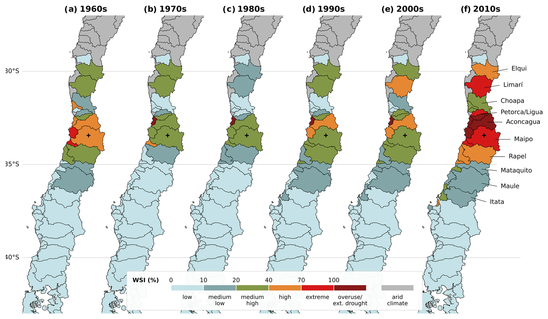
Figure 6 Decadal mean Water Stress Index (WSI) for the major watersheds in central Chile between 1960 and 2020. The names of the basins analyzed further are indicated in the right-hand panel. The cross indicates the location of Santiago city.

By contrast, in the 2010–2020 decade, the combination of low water availability caused by the megadrought and higher water use rates led to a sharp increase in water stress levels in most basins of central-north Chile. During this period, the Maipo River basin reached an extreme water stress level, while other basins, such as La Ligua and Aconcagua exhibited critical levels, with WSI values exceeding 100 %, indicating that water use surpasses available surface water. These elevated water stress levels have been associated with unsustainable use of groundwater reserves, as evidenced by sustained water table declines in this region (Alvarez-Garreton et al., 2024; Jódar et al., 2023; Taucare et al., 2024).

The Aconcagua River basin represents a case of extreme water stress. In this watershed, covering about 7300 km², urban and rural areas coexist alongside multiple productive activities with high and increasing water consumption, sometimes surpassing surface water availability (Fig. 7). Another indication of water demand pressure in this basin is the present-day small gap between the estimated water use and the legal withdrawal limit according to the total WURs (red bars and black curve in Fig. 7a). As in other regions with natural water limitations, Aconcagua's supplies rely heavily on reservoirs and groundwater withdrawals (the groundwater to total WURs ratio currently reaches about 80 %).

During the decades before the megadrought, consumptive water uses in Aconcagua represented about 40 % of the water availability in the basin, indicating a medium to high level of water stress. The water use to availability ratio narrows during periods of drought, as observed during the second half of the 1960s and the recent megadrought (2010–2020), where the 5-year mean WSI exceeded 65 % (high to extreme water stress) and 100 % (a critical condition), respectively.

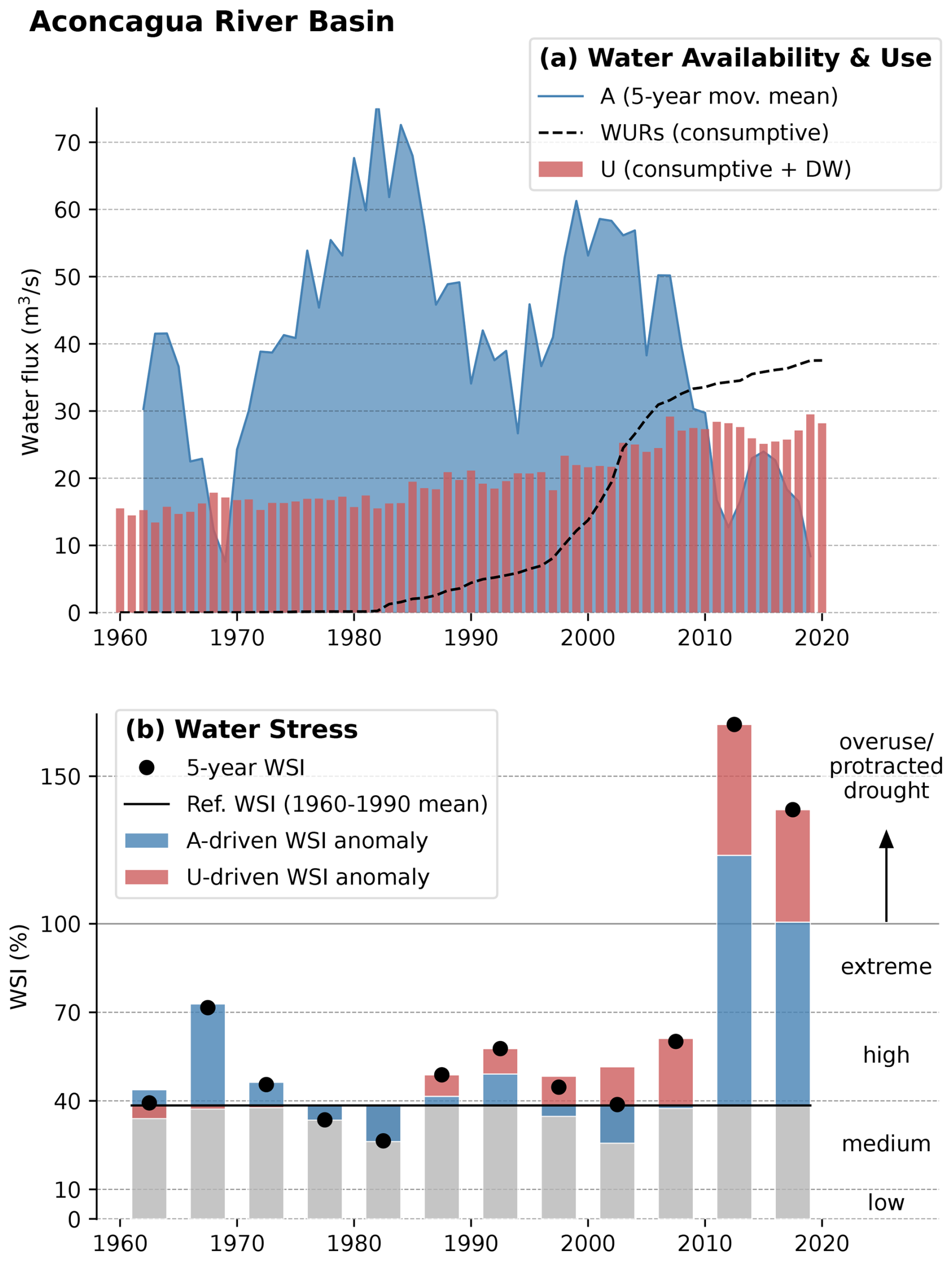
Figure 7 (a) Water availability (A, blue), consumptive water uses (U, red) and rights (WURs, black) in the Aconcagua River basin from 1960 to 2020. (b) Five-year Water Stress Index (WSI) averages in the basin (black dots). Anomalies for each quinquennium relative to the 1960–1990 mean are highlighted in color. The WSI anomalies are disaggregated into two components related changes in water availability (blue) and changes in water use (red).

The primary role that climate variability plays in WSI is evident in the case of the Aconcagua River basin, as shown by quinquennial WSI anomalies attributed to changes in water availability (blue bars in Fig. 7b). However, it is also clear that, in addition to the increased WSI during periods of precipitation deficits, the long-term growth in water use has progressively increased water stress between 1960 and 2020 (red bars in Fig. 7b). Particularly, the increased water use amplified stress levels during 2010–2020, intensifying the impact of the megadrought on water resources.

As in Aconcagua, the increase in water demand since the 1960s has narrowed the gap between availability and use, leading to a substantial rise in water stress levels in most basins in central Chile. The 30-year mean WSI for the period 1990–2020 reflects this condition (Fig. 8). Compared with the previous 30-year period (1960–1990), the WSI increase is mainly associated with the growth in water demand and, to a lesser extent, with the long-term decrease in water availability between the two periods (see red and blue bars in Fig. 8).

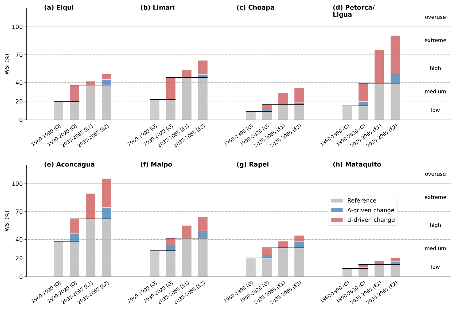
Figure 8 Mean WSI for the periods 1960–1990, 1990–2020 and 2035–2065 in the major basins of central Chile. Changes in WSI compared to a reference period (black line), and the components related to water availability and water use are highlighted in blue and red, respectively. The WSI for the two historical periods are based on actual water use/availability estimates (O). Water availability projections for the mid-21st century are based on 11 ESM simulations (showing the multi-model mean) and two socioeconomic scenarios: one with high (E1, SSP1-RCP2.6) and the other with low (E2, SSP3-RCP7.0) global greenhouse gas emission mitigation. Water use projections assume a linear extrapolation of the trend observed between 2000 and 2020.

Water stress levels in central Chile are projected to worsen in the future due to the continuous decline in water availability and the potential strengthening of this trend under unfavorable climate scenarios (Fig. 8). The water availability decline is primarily attributed to lower precipitation rates and, to a lesser extent, to increased evapotranspiration caused by higher temperatures (not shown). As mentioned in Sect. 3, climate projections involve various sources of uncertainty, and the actual future conditions will depend on the global climate change scenario and regional sensitivity to large-scale climatic disturbances. However, climate model projections consistently show a direction of change towards lower precipitation in central Chile (Fig. 3), leading to high and extreme WSI values in the mid-21st century in the basins of the Elqui, Limarí, Petorca/La Ligua, Aconcagua, and Maipo rivers (Fig. 8). This result considers only changes in water availability under a future climate scenario with a pathway (greenhouse gas increase) similar to one of the recent decades (SSP3-7.0). A further discussion regarding future trends and mitigation options to reduce water stress in Chile is presented next.

6 How to advance toward water security goals?

Given the limited control that local governance and actions have over global climate evolution and considering the precautionary principle regarding climate and water availability projections (e.g., Martin, 1997; Costa, 2014; MMA, 2022), the effects of water demand on the evolution of water security are particularly relevant in Chile.

As seen during the megadrought, increased water stress under unfavorable future climate conditions could be largely exacerbated if water demand continues to rise in basins at high risk of scarcity. To evaluate this threat, along with climate projections, a simple future scenario of water use to the mid-21st century was considered based on recent trends (2000–2020) extrapolation. Under these conditions, several basins are projected to reach extreme levels of water stress, in some cases exceeding the threshold of physical sustainability (WSI >100 %, Fig. 8). WSI values near or above 100 % indicate a structural condition of water overuse with major social and environmental impacts, including even greater pressure on groundwater reserves, as Alvarez-Garreton et al. (2024) reported.

In addition to the projected decline in precipitation and in freshwater availability, a warmer climate will reduce the snow accumulation capacity of headwater basins in central Chile, leading to lower meltwater flows during the summer, when agricultural water demand is highest (Vicuña et al., 2011; Stehr and Aguayo, 2017; Bozkurt et al., 2018; Alvarez-Garreton et al., 2023b; Vásquez et al., 2024). This scenario highlights risk to water security, food security, and socio-economic stability in the region. Similar risks are faced by mountainous regions worldwide that rely on snow-dominated headwater basins (Drenkhan et al., 2023; Adam et al., 2009).

Public policy in Chile increasingly recognizes the impacts of droughts and the challenges that climate change poses to water security. In particular, the Framework Law on Climate Change (MMA, 2022) establishes a set of legal instruments and adaptation plans, many of which are under development at the time of writing this paper. However, some of these instruments – explicitly oriented towards water resources and water security goals (MOP and DGA, 2024) – have not yet defined quantitative metrics of water security.

In our opinion, metrics such as the water stress index assessed in this study are necessary to establish water security goals and to monitor the effectiveness of actions taken to achieve them. One advantage of using the WSI is that stress levels can be associated with water scarcity and environmental risks (e.g., Falkenmark et al., 2007), thereby enabling the definition of specific water security targets. Of course, other metrics are also needed, as the WSI cannot capture the full complexity of water security, which also includes factors such as water quality and accessibility, groundwater depletion, governance, and integrated water resources management, among others. Nevertheless, the WSI offers a clear and straightforward metric that can be effectively complemented by additional indicators.

Given a global climate scenario and its regional manifestation, there are only two ways to reduce the WSI in a basin: by decreasing consumptive water use or by increasing water availability through alternative sources. If public policy establishes a target of, e.g., reaching WSI values of 40 % or lower by 2050, different actions to adjust water availability and demand could help achieve this goal. As an illustrative example, we look at different cases leading to that target in the Aconcagua River basin, considering the basin history and the climate projections assessed in this study (Fig. 9 and Table 2). The consumptive water use in the basin nearly doubled over the past six decades, primarily due to the growth of irrigated agriculture (Fig. 9). A period of large water availability in the 1980s, along with international trading opportunities, encouraged policy decisions aimed at boosting agricultural development and positioning Chile as a global food-exporting leader (Villalobos et al., 2006). However, the onset of the megadrought and the climatic projections for the region question the feasibility of sustaining these consumption levels if water security is to be achieved.

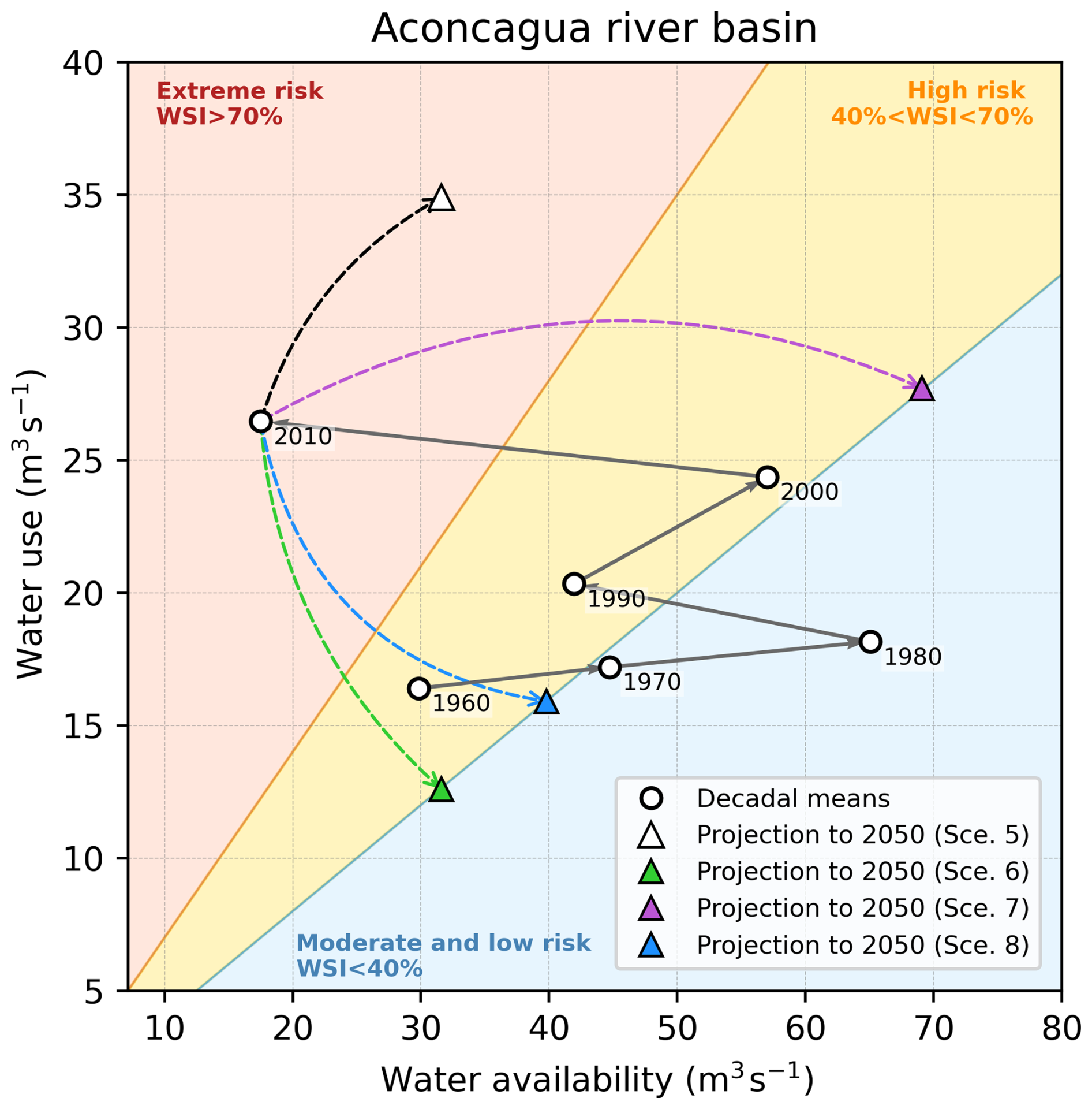
Figure 9 The decadal evolution of consumptive water use, water availability, and the corresponding WSI category (background) in the Aconcagua River basin for the period 1960–2020 (circles). Triangle markers indicate different scenarios for the mid-21st century under a global climate scenario with low greenhouse gas emission mitigation (SSP3-7.0, scenarios 5 to 8 in Table 2).

Different pathways to meet the water security target (WSI <40 %) by 2050 in the basin are presented in Table 2, including extreme cases where the target is met either by exclusively reducing water use (scenarios 2 and 6 in Table 2) or by solely increasing water availability (scenarios 3 and 7) through engineering solutions, such as inter-basin water transfers or seawater desalination. In the first case, adjustment measures would need to substantially reduce consumptive uses (by nearly 50 % under unfavourable climate conditions). In the second case, alternative sources would need to increase water availability by 35 m³ s⁻¹, that is, doubling the natural availability in Aconcagua.

Table 2 Projected WSI for the mid-21st century (2035–2065) in the Aconcagua River basin under different scenarios of climate and related water availability (A_C), alternative water availability sources (A_A), such as seawater desalination or inter-basin transfer, and consumptive water use (U_CO). Relative changes compared to the reference period 1990–2020 are provided in parentheses. Projections of A_C based on eight ESM simulations and two socio-economic scenarios: one with high global mitigation of greenhouse gas emissions (SSP1-RCP2.6) and another with low mitigation (SSP3-RCP7.0).

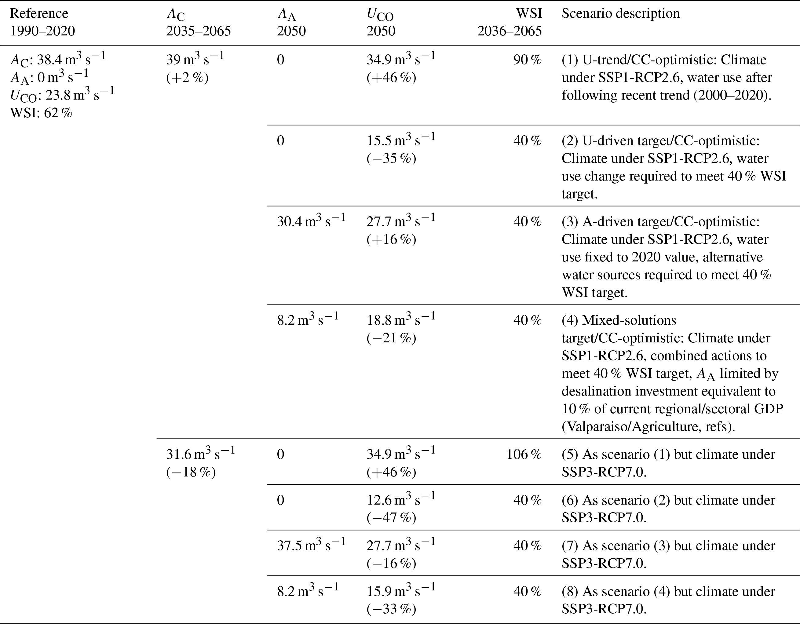
Both solutions involve socio-economic and environmental costs that should be carefully assessed. The best approach will likely involve combined efforts. Desalination has rapidly developed in Chile and is projected as a key solution for mitigating risks to basic water provision and industry in northern Chile (Vicuña et al., 2022). However, given the current energy, economic, and environmental costs, the expansion of this technology to supply high water-demand sectors such as agriculture still seems distant. As a rough estimate, considering only the economic cost and assuming a very low production rate of desalinated seawater (USD 0.25 m⁻³; about half of the lowest published costs; Vicuña et al., 2022), an annual investment of USD 65 million, equivalent to 10 % of the GDP of the agricultural sector in Valparaiso (the administrative region that houses the Aconcagua basin), would lead to a water flux of about 8 m³ s⁻¹. Even with this alternative water source, consumptive water use would still need to be reduced by 20 % to 35 % to achieve the target of a 40 % WSI by mid-21st century, depending on the climate trends (Table 2). These values can serve as benchmarks for further in-depth assessments of actions focused on climate change adaptation and on mitigating the water use impacts of current land use activities.

It is important to distinguish between total and consumptive water uses when considering alternatives to reduce water stress, particularly in the design of water use efficiency plans. Irrigation strategies can alter how water is used in a watershed by either redistributing it more effectively or by reducing plants' consumptive water use. In the first case, studies have shown that it is possible to reduce irrigation by 20 % in table grape crops while maintaining transpiration and reducing percolation, thereby avoiding negative impacts on water quality, such as the transport of agrochemicals to groundwater (Pizarro et al., 2022). This approach reduces total water use, but not consumptive use. In the second case, a 25 % to 30 % reduction in transpiration can be achieved through controlled plant stress management, as demonstrated locally in avocado cultivation (Beyá-Marshall et al., 2022). However, these management strategies can only reduce basin-scale water stress if they result in a reduction in total consumptive water use (Grafton et al., 2018).

It should be noted that non-renewable water reserves, such as aquifers that are not in equilibrium or melting glaciers, are not considered as alternative sources to reduce the WSI. These water reserves, along with those from artificial reservoirs, play a key role in water security primarily through temporal regulation and water accessibility. However, they do not represent a long-term additional source of water since their storage is limited by surface recharge rates. Given this limitation, water consumption at rates close to or exceeding surface availability will not be sustainable over time, regardless of whether the access is from underground, surface sources, or reservoirs (Alvarez-Garreton et al., 2024).

7 Conclusions and recommendations

This paper offers a comprehensive evaluation of Chile's current, historical, and future water stress conditions, utilizing novel datasets on water availability and use. These datasets address critical information gaps in Chile and are relevant for various applications, including climate, land use, and water management.

We highlight the following conclusions from this study:

1. Most basins in central Chile experienced high to extreme water stress between 2010 and 2020. This situation was primarily driven by reduced precipitation and water availability during this period (megadrought) and was further exacerbated by high water demand in the region.

2. From a historical perspective, water stress has steadily increased over the last six decades in central Chile, leading to permanent (30-year mean) high levels of water stress (WSI >40 %) in several basins from Santiago to the north. This increase is mainly attributed to rising water consumption and, to a lesser extent, to a reduction in surface water availability. During this period, consumptive water use in the country has doubled, largely due to the expansion of the agricultural and forestry industries.

3. In a scenario of adverse climate change, conditions similar to those of the megadrought are projected to become permanent by the end of the 21st century, with nearly a 30 % reduction in precipitation. Under such circumstances, most basins in the central and northern regions of the country are likely to experience persistently high or extreme levels of water stress by the mid-21st century.

Following the scientific evidence provided here and in other studies, we recommend decision-makers and water users to acknowledge that Chilean regulations have permitted and continue to allow consumptive water uses that exceed recognized sustainability levels in the central-northern regions of the country. Renewable water availability supports ecosystems and society for long-term functioning. Natural water reserves, such as aquifers, snow, and glaciers, as well as artificial reserves like reservoirs, complement water availability, mainly by providing temporal regulation. These storage systems enable access to greater water volumes, though this is limited by surface recharge rates. Given this limitation, water uses that approach or exceed renewable water availability will not be sustainable over time, whether the water is accessed through groundwater, surface water, or reservoirs.

Based on this understanding, measures can be evaluated and agreed upon to mitigate the impact of high water consumption activities. These actions should be implemented alongside effective adaptation strategies to address current and future climate trends, particularly concerning the impacts on the Andes Cordillera. Over this region, future scenarios of water stress will be likely exacerbated by reductions in snow accumulation driven by rising temperatures, resulting in diminished meltwater flows from headwater basins during summer, when agricultural water demand is at its peak.

The analysis of water use pathways and alternative sources to achieve water security under climate change – illustrated here by targeting a WSI below 40 % by 2050 – offers valuable input for ongoing adaptation planning. While setting basin-specific WSI thresholds and strategies to meet them falls within the scope of public policy, adopting this index can facilitate discussions on the main approaches to achieving the target: either reducing water use or increasing availability through alternative sources.

We recommend that current adaptation plans define goals based on basin-scale water balance indicators, such as the WSI, complemented by additional metrics that capture other key dimensions of water security (e.g., water access and equity, groundwater depletion, ecological flow requirements, among others). A comprehensive set of water security indices is essential for evaluating adaptation strategies; however, a key challenge lies in making the political decisions to set targets for these indices and to determine the necessary changes and associated costs to achieve them.

The methods used in this study can be applied to any region that meets the necessary data requirements. The estimates of water availability, water use and stress presented here carry uncertainties related to climate, hydrological, and land cover data that should be contrasted and complemented with independent approaches. Monitoring key variables related to water security and facilitating access to data, particularly from public agencies, is also crucial for a comprehensive assessment of water stress and effective planning.

Appendix A: Evapotranspiration model

An evapotranspiration (ET) model was developed to assess changes in water availability and estimate water use in the LULUCF sector across Chile. This model employs a bucket scheme, like those used in many surface or hydrological models (e.g., Sellers et al., 1997). The model includes a soil water reservoir, replenished by precipitation (P) up to its maximum capacity and depleted through ET. The ET flux scales linearly with the soil water content and is limited by a maximum ET ratio relative to potential evapotranspiration (ET₀), defined by a parameter β_X. Like crop coefficients, β_X represents plants' inherent transpiration (T) intensities in the absence of moisture stress, reflecting canopy conductance and other physiological/morphological properties that affect the water use efficiency of different functional types. Intercepted precipitation in the vegetation canopy is explicitly accounted for through a secondary small tank, leading to evaporation (E_I) with no limitations other than ET₀ and the available canopy water (as a water body).

The model runs on a daily time step following these main equations:

$$\begin{array}{}\text{(A1)}& {\displaystyle }\begin{array}{rl}\text{ET}(x,t)& =a\left[E_{\mathrm{I}}\right(x,t)+f_{\mathrm{IWB}}{\text{ET}}_{\mathrm{IWB}}(x,t)\\ & +(\mathrm{1}-f_{\mathrm{IWB}}){\text{ET}}_{\mathrm{ML}}(x,t)]\end{array}\text{(A2)}& {\displaystyle }{E}_{\mathrm{I}}(x,t)=min\left[\mathrm{1.2}{\text{ET}}_{\mathrm{0}}\right(x,t),W_{\mathrm{I}}(x,t\left)\right]\text{(A3)}& {\displaystyle }{\text{ET}}_{\mathrm{IWB}}(x,t)={\mathit{\beta }}_X{\text{ET}}_{\mathrm{0}}(x,t)\text{(A4)}& {\displaystyle }{\text{ET}}_{\mathrm{ML}}(x,t)=min\left[\mathit{\beta }\right(x,t\left){\text{ET}}_{\mathrm{0}}\right(x,t),W_{\mathrm{S}}(x,t\left)\right].\end{array}$$

For a given location or grid cell (x) and time step (t), the main output in Eq. (A1) represents an ET flux (in mm d⁻¹) composed of E_I and two fluxes computed under unlimited (ET_IWB) and limited (ET_ML) soil moisture conditions. The relative importance of ET_IWB and ET_ML is controlled by fraction f_IWB, which serves as an activation flag for irrigated areas or water bodies. Factor a adjusts each component proportionally to limit ET to a maximum rate of 1.2 ET₀ (i.e., a is the ratio between this maximum value and the sum of the bracketed components in Eq. (A1), or is set to one if the sum does not exceed the limit). The factor of 1.2 defines the maximum possible ET flux, such as in open water conditions (ET₀ estimates used here stand for a reference ET over grass, to which a scaling is applied following Finch and Hall, 2001). The interception component E_I (Eq. A2) is a flux of maximum evaporation constrained by the canopy reservoir W_I. ET_IWB is only limited by β_X, while ET_ML is constrained both by β_X and the soil water content (W_S) through coefficient β:

$$\begin{array}{}\text{(A5)}& \mathit{\beta }(x,t)={\mathit{\beta }}_X{\displaystyle \frac{W_{\mathrm{S}}(x,t)}{w_{\mathrm{S}X}\left(x\right)}}\end{array}$$

where w_SX represents the water capacity of the soil tank, which depends on a rooting depth parameter (d_R) and a fraction of available water capacity (AWC), as follows:

$$\begin{array}{}\text{(A6)}& w_{\mathrm{S}X}\left(x\right)=\text{AWC}\left(x\right)d_{\mathrm{R}}.\end{array}$$

While d_R is prescribed for a given land cover class, AWC varies spatially according to soil texture and bulk density. In this study, AWC was derived from the latter properties for six soil layers (0–5, 5–15, 15–30, 30–60, 60–100 and 100 to 200 cm) using the Rosetta V3 pedotransfer functions (Zhang and Schaap, 2017), and it is provided by CLSoilMaps, a database of gridded physical and hydraulic soil properties for Chile (Dinamarca et al., 2023; Galleguillos et al., 2024). Consequently, the model does not use a fixed soil layer depth. Instead, it employs the effective soil bucket capacity (w_SX), which depends on the hydraulic properties of a given location (AWC) and the rooting depth (d_R) of a specific vegetation type.

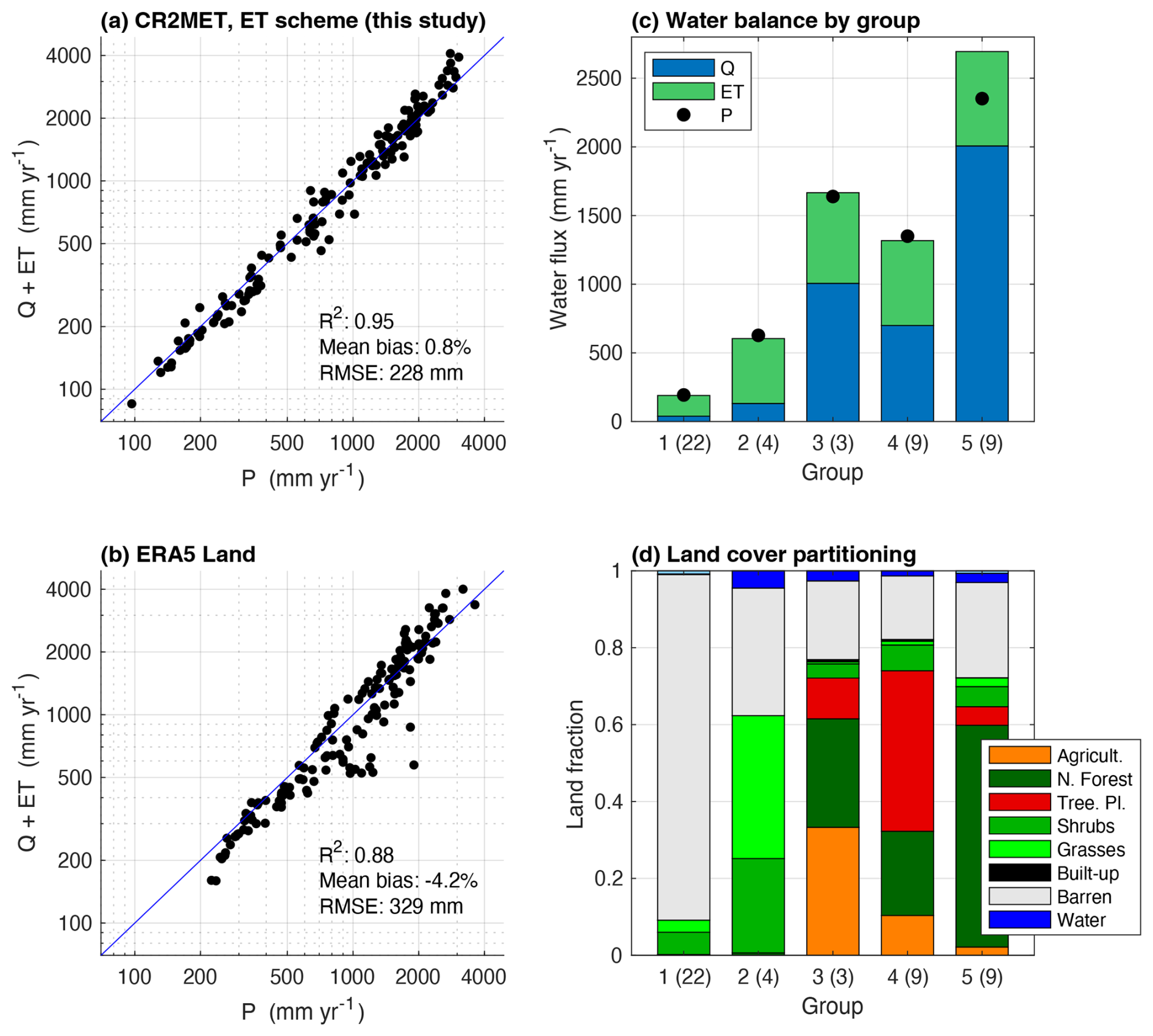
Figure A1 Comparison of mean annual precipitation (P) in 147 watersheds in Chile with observed river streamflow (Q) and modeled evapotranspiration (ET). The estimates of P and ET in panels (a) and (b) correspond to those assessed in this study (CR2MET-driven) and from ERA5-Land, respectively. Panel c shows the CR2MET-based flux comparison for groups of watersheds with dominant fractions of barren land (>85 %, group 1), shrubland and grasses (>40 %, group 2), agriculture (>30 %, group 3), tree plantations (>30 %, group 4), and native forest (>50 %, group 5). The number of basins and mean land cover partitioning of each group is shown in panel (d).

Based on previous conditions, at the beginning of each time step, water reservoirs are partially or totally filled by fractions of total precipitation, which are allocated to the canopy (P_I, interception) and soil (P_S) components as:

$$\begin{array}{}\text{(A7)}& {\displaystyle }{P}_{\mathrm{I}}(x,t)=min[w_{\mathrm{I}X}-W_{\mathrm{I}}(x,t-\mathrm{1}),P(x,t\left)\right]\text{(A8)}& {\displaystyle }\begin{array}{rl}{P}_{\mathrm{S}}(x,t)=min& \left[w_{\mathrm{S}X}\right(x)-W_{\mathrm{S}}(x,t-\mathrm{1}),\\ & P(x,t)-P_{\mathrm{I}}(x,t)]\end{array}\end{array}$$

where w_IX stands for water holding capacity of the canopy. The remaining precipitation ($P-P_{\mathrm{I}}-P_{\mathrm{S}}$) is considered as the model runoff. At the end of each cycle, the soil and canopy reservoirs are partially emptied following the ET_ML and E_I losses, respectively.

Hence, in addition to the forcing and internally computed variables, four parameters control the model: the coefficient β_X (dimensionless), the rooting depth d_R (mm), the canopy interception capacity w_IX (mm) and the saturation fraction f_IWB (boolean). Water fluxes and storages defined by Eqs. (A1) to (A8) are calculated independently for different land cover conditions, each with its own set of parameters (Table S2 in the Supplement). The final ET flux is determined as a weighted average across the various land cover types coexisting in a spatial unit (grid cell), using a mosaic approach like that employed in several land surface models (e.g., Blyth et al., 2021). For the purposes of this study, the model runs in a fully distributed manner over the domain and with the spatial resolution defined by the atmospheric forcing CR2MET (continental Chile, 0.05° latitude-longitude grid), and using the 48 land cover classes included in CR2LUC.

Soil evaporation is not explicitly included in Eq. (A1) but is accounted for through the flux ET_ML as an independent tile. The fractional area of this tile results from the barren land fraction prescribed in CR2LUC (code 600) and the residual fraction from the effective coverage ($F_K^{\left(\mathrm{eff}\right)}$) of other classes. In a similar approach to other models (e.g., Krinner et al., 2005), the fraction $F_K^{\left(\mathrm{eff}\right)}$ reduces the area prescribed for vegetated classes (F_K) based on its canopy cover, thereby accounting for differences in foliar density and the phenological cycle of plants. This is modeled following the Beer-Lambert law:

$$\begin{array}{}\text{(A9)}& F_K^{\left(\mathrm{eff}\right)}(x,t)=F_K(x,t)(\mathrm{1}-e^{-\mathrm{0.6}{\text{LAI}}_K\left(t\right)})\end{array}$$

where LAI_K is the Leaf Area Index of a vegetation class K. The factor 0.6 has been chosen as a typical value for the light extinction coefficient (e.g., van Dijk and Bruijnzeel, 2001). Consequently, the actual grid area fraction of a vegetated class seen by the model will range between 0 and a value that tends to F_K for elevated LAI. In this study, we computed the monthly mean LAI (2014–2019) for each vegetated class based on the 333 m PROBA-V LAI satellite dataset from the Copernicus Global Land Service (CGLS; Smets et al., 2018). The data were processed for equivalent grid cells with a dominant fraction of the corresponding CR2LUC class, using data sources from this product (Sect. 2.4), particularly the fruit cadastres from ODEPA, the vegetation cadastres from CONAF, and the 30 m Land Cover for Chile (Zhao et al., 2016).

The main objective of this scheme is to accurately represent the ET mean rate, its seasonal and long-term variability, rather than modeling runoff as in a full hydrological model. As such, snow accumulation and melt are not included, nor are any processes related to runoff propagation. Sublimation over permanent snow/glacier conditions is accounted for in the same way as ET in other land cover types, with its own set of parameters. With these limitations, the model does not fully capture runoff seasonality and variability, especially in mountain watersheds influenced by snow. However, the long-term mean runoff within watersheds were contrasted with observed river streamflows to adjust parameters and validate water balance of the model.

Land cover classes included in CR2LUC, along with the set of parameters used in this study, are listed in Table S2. Most parameters were based on published data. Rooting depth values vary greatly depending on the metric used, such as maximum depths or percentiles in vertical root distribution (e.g., Canadell et al., 1996; Schenk and Jackson, 2002). For agricultural classes, we prescribed the maximum effective rooting depth as specified in the Food and Agriculture Organization's Irrigation and Drainage Paper No. 56 (FAO56; Allen et al., 1998), similar to the values of maximum rooting depths reported by Fan et al. (2016). For natural vegetation and tree plantations, prescribed rooting depth values range from 0.3 m (Tundra) to 3.0 m (sclerophyllous and eucalyptus trees), based on the data from Canadell et al. (1996), Schenk and Jackson (2002), Fan et al. (2017) and Tumber-Dávila et al. (2022).

Parameter w_IX varies between 0.3 and 2 mm. For agricultural classes, the values were derived using the model of van Dijk and Bruijnzeel (2001) with the leaf and stem water capacity from Zhong et al. (2022), and the LAI data described earlier. For natural vegetation and tree plantations, we used the storage capacity per unit of canopy area, also based on Zhong et al. (2022).

For β_X, we adopted the mid-season crop coefficients from FAO56 for agricultural classes, ranging from 0.7 to 1.2. Setting β_X for natural classes and tree plantations is not straightforward. In this case, we were guided by published observations-based data on ET $/$ ET₀ ratios (Liu et al., 2017b), ET $/$ P ratios (White et al., 2022; Balocchi et al., 2023), and T $/$ ET ratios (Schlesinger and Jasechko, 2014; Benyon and Doody, 2015; Nelson et al., 2020). However, this information serves only as a reference since these quantities are influenced by factors such as moisture stress, leaf area, and intercepted evaporation, which do not precisely correspond to the unstressed T $/$ ET₀ rates accounted for by β_X. In general, we aimed to maintain differences between functional types (e.g., shrubs vs. trees, broadleaf vs. needleleaf), but the final β_X values were calibrated by assessing the water balance in basins with monitored streamflow and distinct land covers (Fig. A1), resulting in values ranging from 0.5 to 0.9.

Non-vegetated classes were also characterized through these parameters. For barren land and built-up areas, topsoil layers of 200 and 50 mm were assigned, respectively. Additionally, a w_IX value of 1.0 mm was included for the latter to account for intercepted water on impervious surfaces. Water bodies evaporate at maximum rates (β_X=1.2), except for wetlands and salt pans, which are only partially covered by saturated areas. Sublimation from glaciers and permanently snow-covered areas was modeled as water bodies with limited evaporation rates (β_X=0.2), mimicking the ET $/$ ET₀ ratios shown by ERA5 land over glacier areas, such as in the Patagonian Ice Fields.

Figure A1 presents a validation summary of the ET simulations. We used the CAMELS-CL dataset (Alvarez-Garreton et al., 2018) to compare long-term (1990–2020) average river streamflows (Q) observed in Chile with watershed-averaged P and ET. A total of 147 basins were selected based on data availability (at least 75 % coverage during 1990–2020) and the absence of disturbances significantly affecting river discharges. The sum of the observed Q and simulated ET shows a strong inter-basin correlation with the CR2MET P (R²=0.95) and exhibits low overall bias (<1 %). More noticeable and systematic biases, where Q+ ET values exceed P, are found in humid watersheds (P>2000 mm yr⁻¹). We attribute these biases primarily to an underestimation of CR2MET P rather than an overestimation of ET, since the latter is mostly limited by ET₀ and the runoff coefficients ($Q/P$) in these watersheds approach or even exceed 100 %. These basins are predominantly covered by native, temperate rainforest. Aside from this group, there is no systematic bias across other watersheds with distinct land cover (Fig. A1c).

For benchmarking, we conducted the same analysis using independent P and ET data from ERA5-Land reanalysis (Muñoz-Sabater et al., 2021), which yielded poorer results (Fig. A1b), highlighting the added value of these new datasets for Chile.

Appendix B: Near-present water use in Chile – data source comparison

Table B1 Sectoral water use in continental Chile (km³ yr⁻¹) from different estimates. Where available, values are classified as consumptive and non-consumptive.

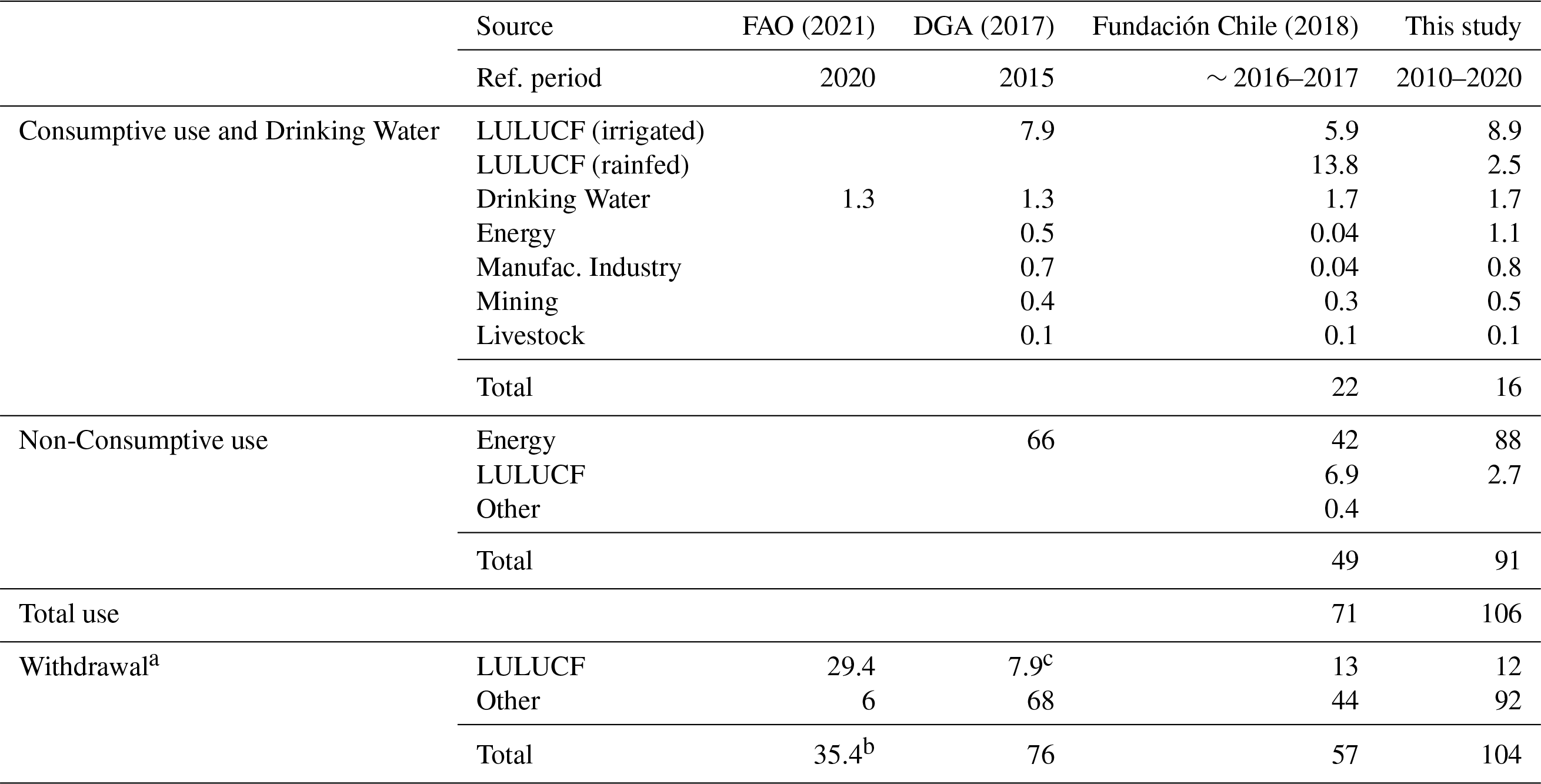
^a Blue water withdrawals (exclude rainfed agriculture). ^b FAO-AQUASTAT's Total Freshwater Withdrawal. It does not account for withdrawals in hydropower generation. ^c Does not account for non-consumptive water use in agriculture.