Soil moisture and precipitation intensity jointly control the transit time distribution of quick flow in a flashy headwater catchment

The rainfall–runoff transformation in catchments usually follows a variety of slower and faster flow paths, leading to a mixture of “younger” and “older” water in streamflow. Previous studies have investigated the time-variable distribution of water ages in streamflow (transit time distribution, TTD) using stable isotopes of water (δ¹⁸O, δ²H) together with transport models based on StorAge Selection (SAS) functions. These functions are traditionally formulated based on soil moisture to mimic the preferential release of younger water as the system becomes wetter. In this study, we hypothesized that, in a heterogeneous catchment with a significant fast-runoff response component, precipitation intensity, in addition to soil moisture, plays a critical role in the preferential release of younger water. To test this hypothesis, we used high-resolution δ¹⁸O data (weekly and event-based streamflow δ¹⁸O samples) in a 66 ha agricultural catchment. We tested two scenarios of the SAS function parameterization for the preferential-flow age selection: one as a function of soil moisture only and one as a function of both soil moisture and precipitation intensity. The results showed that accounting for both soil moisture and precipitation intensity to define the shape of SAS functions for preferential flow improved the tracer simulation in streamflow (increasing the Nash–Sutcliffe efficiency from 0.31 to 0.51). This also led to a higher percentage of streamflow (an increase from 2.87 % to 4.38 %) with shorter transit times (TTs younger than 7 d), with the largest differences occurring during the summer and autumn months. This was due to the fact that incorporating both soil wetness and precipitation intensity in the SAS formulation accounts for rapid flow pathways such as infiltration excess overland flow, preferential flow through macropores, and tile drain flow – allowing precipitation water to bypass much of the soil matrix and to reach the stream with minimal storage or mixing, even under dry soil conditions. We showed for the agricultural study catchment that a significant portion of event water bypasses the soil matrix through fast-flow paths, resulting in younger water reaching the stream for both low- and high-intensity precipitation. Thus, in catchments where preferential flows and overland flow are the dominant flow processes, soil-wetness-dependent and precipitation-intensity-conditional SAS functions may be required to better describe the timescale of solute transport in modelling, which has implications for stream water quality and agricultural management practices such as the timing of fertilizer application.

1 Introduction

The focus of hydrological research has expanded from the quantitative estimation of water fluxes to better descriptions of underlying hydrological processes by estimating the water age of various storage and runoff components in catchments (Beven, 2006; McDonnell and Beven, 2014; Sprenger et al., 2019). Water age provides crucial information about the pathways through which water moves in catchments. This information can be used to quantify the timescale of the flow of precipitation through different pathways such as overland flow, lateral subsurface flow, and deep percolation. Such knowledge is useful for quantifying the fate of pollutants and sediments in catchments, which is essential for maintaining stream water quality and ensuring sustainable management of water resources.

The time it takes for precipitation to reach the stream is referred to as the water transit time, while water age is the time that has elapsed since precipitation entered the catchment (Rinaldo et al., 2011; Botter et al., 2011; Benettin et al., 2022). Depending on the physical characteristics of a catchment and on the hydrometeorological conditions, transit times can vary from seconds to decades. Therefore, the knowledge of water transit time and its distribution (TTD) is essential for characterizing transport processes in catchments (McGuire and McDonnell, 2006; Botter et al., 2011; Klaus and McDonnell, 2013; Benettin et al., 2022). Despite their usefulness in studying water flow through catchments, transit time (TTs) cannot be measured directly on a catchment scale, and they are instead inferred from catchment-wide input–output signals, for example, by using the stable isotopes of oxygen (δ¹⁸O) and hydrogen (δ²H) in precipitation and streamflow (Kirchner et al., 2000; Fenicia et al., 2008, 2010; McGuire and McDonnell, 2006; Klaus and McDonnell, 2013; McDonnell and Beven, 2014; Benettin et al., 2022; Wang et al., 2025). δ¹⁸O and δ²H have been widely used to estimate the water transit times of precipitation parcels into different hydrological fluxes such as root water uptake; plant transpiration; lateral subsurface flow; and, eventually, streamflow (Hrachowitz et al., 2015; Abbott et al., 2016; Knighton et al., 2019, 2020; Kübert et al., 2023).

Recent advances in sampling techniques now enable high-resolution stable isotope measurements, including hourly δ¹⁸O of precipitation (von Freyberg et al., 2022) and sub-daily to daily δ¹⁸O of streamflow (von Freyberg et al., 2022). Building on these data, several tracer-aided hydrological models have been developed to investigate the contributions of distinct runoff generation mechanisms by simultaneously solving water, tracer, and water age balances (Botter et al., 2011), thereby providing estimates of water transit times (Hrachowitz et al., 2013; Benettin et al., 2015; Lutz et al., 2018; Kuppel et al., 2018; Remondi et al., 2019; Wang et al., 2023), as well as estimates of the temporal variability in runoff generation processes (Kirchner et al., 2000; Fenicia et al., 2008, 2010; McGuire and McDonnell, 2006; Klaus and McDonnell, 2013; McDonnell and Beven, 2014; Benettin et al., 2022; Wang et al., 2025).

TTD estimation methods have recently evolved to describe the relationship between water storage and discharge in hydrological systems using the StorAge Selection (SAS) approach (Botter et al., 2011; Rinaldo et al., 2015). The SAS function characterizes the probability of water parcels of different ages in a catchment's storage being released, thereby representing the relative contribution of young and old water to streamflow (Botter et al., 2011; Rinaldo et al., 2015). Since SAS functions cannot be directly observed, they are typically inferred from the calibration of a tracer-aided hydrological model that fits modelled tracer and streamflow signals to observed ones. They can be defined either as time-variable or time-invariable functions (Hrachowitz et al., 2013) with various functional shapes, such as beta (van der Velde et al., 2012), Dirac delta (Harman, 2015), or gamma (Harman, 2015) distributions.

Using SAS functions, previous studies have shown that TTDs are variable across time and space. Further, studies have shown the time variability of SAS functions is controlled by soil moisture (soil storage), thus accounting for the higher probability of releasing a higher percentage of young water as a catchment's soils become wetter (Harman, 2015, 2019; Hrachowitz et al., 2016; Benettin et al., 2017a; Kaandorp et al., 2018). This is sometimes also referred to as the “inverse storage effect” (Harman, 2015). The wetness-dependent time variability of SAS functions has been implemented in hydrological models to simulate tracer fluctuations in streamflow in catchments, such as Claduègne (Hachgenei et al., 2024), Gårdsjön (van der Velde et al., 2015), Elsbeek and Springendalse Beek (Kaandorp et al., 2018), Plynlimon (Benettin et al., 2015; Harman, 2015), and several Scottish catchments (Hrachowitz et al., 2013). This time-variable parameterization of the SAS function depending on catchment wetness may be needed in catchments due to various factors. These factors include (i) the dominance of a single process dependent on soil moisture conditions, such as in the Hafren catchment in Wales (Benettin, et al., 2015; Harman, 2015), or saturation excess overland flow, such as in the Bruntland Burn catchment in Scotland (Benettin et al., 2017a), and (ii) other site-specific hydrological characteristics that may be primarily influenced by catchment wetness.

Although preferential release of younger water is often accounted for in SAS functions through soil-moisture-dependent mechanisms, preferential release of younger water can also occur independently of the soil moisture state when precipitation intensities exceed infiltration capacity. This is particularly critical for catchments where flow generation is not linearly related to soil storage, such as the flashy Weierbach catchment in Luxembourg (Rodriguez and Klaus, 2019), and for catchments where precipitation intensity and duration may play a critical role in how quickly water is mobilized from the landscape due to moderate to low soil infiltration capacity, such as at the Hydrological Open-Air Laboratory in Austria (Vreugdenhil et al., 2022). Exclusively basing the shape of the SAS function on soil moisture may not fully capture the complexity of hydrological responses or all relevant transport processes due to non-linear relationships between storage and streamflow (Danesh-Yazdi et al., 2018; Rodriguez and Klaus, 2019). Therefore, it remains to be tested whether accounting for precipitation intensity in addition to soil moisture to parameterize time-variable SAS functions may yield improved representations of stream tracer dynamics in specific environments.

The objective of this study is to test two alternative approaches to formulate the shape of time-variable SAS functions to account for the higher probability of releasing young water in a flashy headwater catchment: (i) soil moisture exclusively controls the SAS function shape for the preferential release of younger water, and (ii) soil moisture and precipitation intensity jointly control the SAS function shape for the preferential release of young water. We hypothesize that, in a heterogeneous catchment with a significant fast-runoff response component, precipitation intensity, in addition to soil moisture, plays a critical role in the preferential release of younger water to the stream. To test this hypothesis, we used high-resolution δ¹⁸O data (weekly and event-based streamflow δ¹⁸O samples) in the 66 ha agricultural catchment of Petzenkirchen (Hydrological Open-Air Laboratory, HOAL) in Austria. We addressed the following questions:

1. How does formulating the SAS function based solely on soil moisture reflect the streamflow tracer simulation and the inferred transit times?

2. How does formulating the SAS function based on soil moisture conditioned by precipitation intensity affect the streamflow tracer simulation in the catchment and the inferred transit times?

2 Methodology

2.1 Study site

The Hydrological Open-Air Laboratory (HOAL) is a 66 ha site located in Petzenkirchen, Austria (Fig. 1). The catchment is characterized by a humid climate with an average annual air temperature of 9.5 °C. The mean annual precipitation and runoff are 823 and 195 mm yr⁻¹, respectively. The year 2015 was notably dry (P=580 mm yr⁻¹), while 2013, 2014, 2016, and 2017 had higher precipitation levels (>700 mm yr⁻¹) and were classified as relatively wet years. The elevation ranges between 268 and 323 m above sea level, with an average terrain slope of 8 %. The predominant soil types are Cambisols (57 %), Planosols (21 %), Kolluvisols (16 %), and Gleysols (6 %). The soils are characterized by a high clay content of 20 %–30 % (Blöschl et al., 2016; Eder et al., 2014). Land use primarily includes agriculture (87 %) (crop cultivation of maize, winter wheat, rapeseed, and barley), forest (6 %), pasture (5 %), and paved areas (2 %) (Blöschl et al., 2016). A previous study in the catchment showed that the saturated hydraulic conductivity (Ks) exhibits substantial variability despite relatively limited spatial variation in physical and topographical soil properties. In arable fields, median Ks is approximately 3 times higher than in grassland areas, with arable land having a mean Ks of around 47 mm h⁻¹ compared to 20 mm h⁻¹ in grassland. Overall, Ks ranges over 2 orders of magnitude, from as low as 1 mm h⁻¹ to as high as 130 mm h⁻¹, with a coefficient of variation (CV) of around 75 % in arable land (Picciafuoco et al., 2019). The concave part of the catchment (Fig. 1) was tile drained in the 1940s to reduce waterlogging because of the shallow, low-permeability soils and the catchment's use as agricultural land. The estimated drainage area from the tile drains is about 15 % of the total catchment area (Fig. 1).

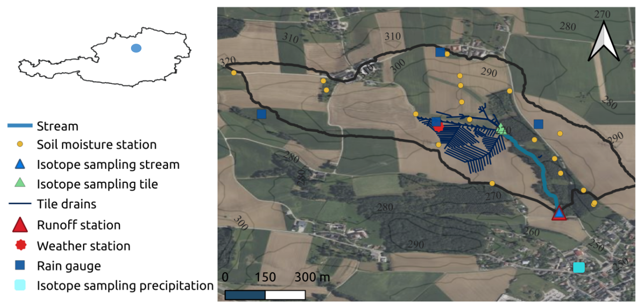
Figure 1 Map of the HOAL catchment (66 ha, lower Austria) and location of rain gauges, a weather station, soil moisture stations, isotope sampling of stream water, and isotope sampling of precipitation (located approximately 300 m south of the catchment, light-blue circle) (map image from © Microsoft, Bing Maps via Virtual Earth).

2.1.1 Hydrometeorological data

Hydrometeorological data for the time period between October 2013 and December 2018 were used for the analyses (Figs. 1 and 2a). Daily precipitation was available from four weighing rain gauges (OTT Pluvio). The arithmetic mean of the four rain gauges was used as the catchment average precipitation. Daily runoff at the catchment outlet was monitored using a calibrated H flume with a pressure transducer. Daily soil moisture in the unsaturated zone was available through 19 permanently installed sensors. The catchment average soil water content was calculated across four different depths: 0.05, 0.10, 0.20, and 0.50 m. Sensor specifications and additional details about the hydrometeorological data are provided in Blöschl et al. (2016).

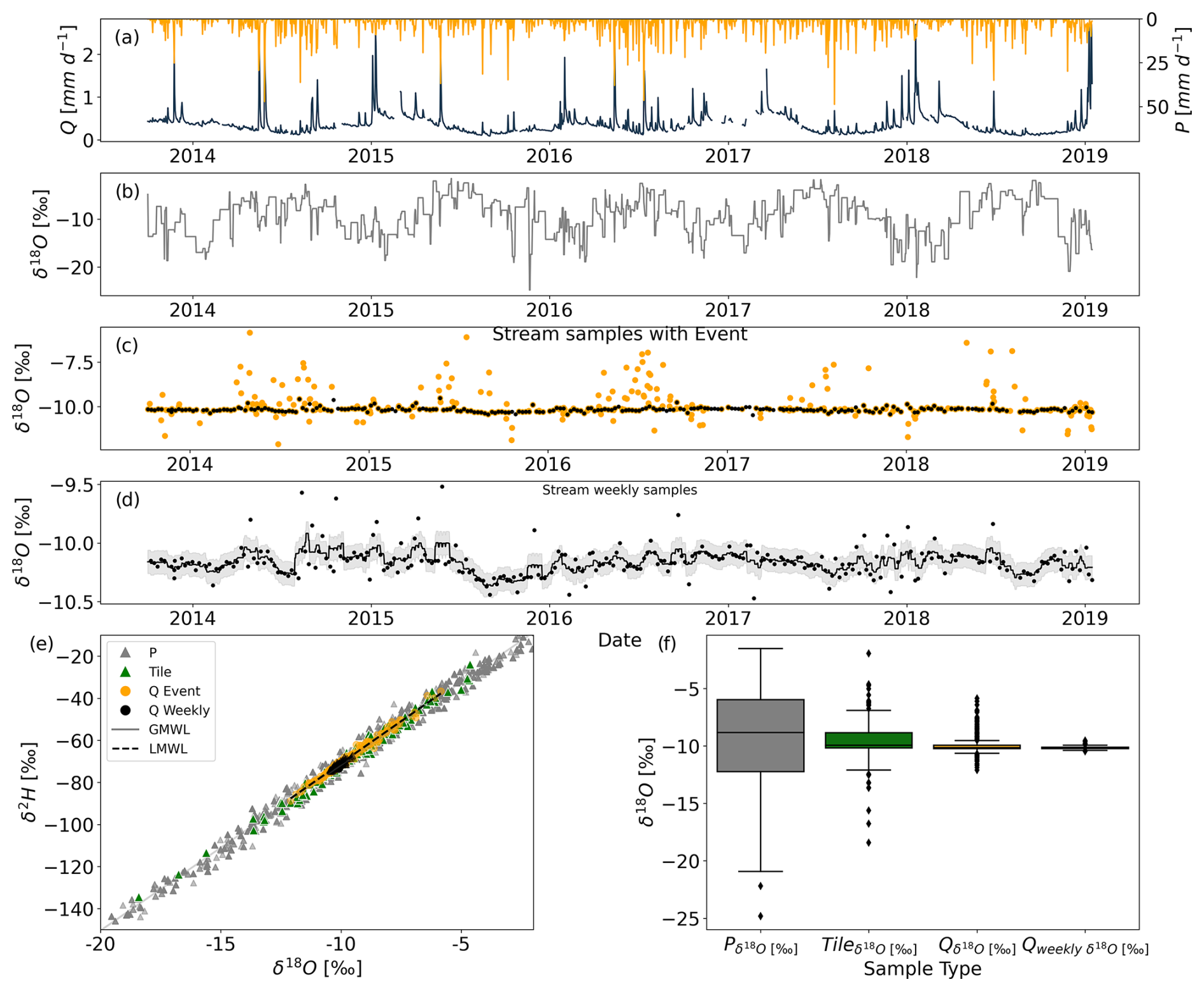
Figure 2 Hydrological and tracer data of the HOAL catchment. (a) Daily observed precipitation P (mm d⁻¹) and streamflow Q (mm d⁻¹); (b) δ¹⁸O data from precipitation event samples at daily timescale; (c) δ¹⁸O data from streamflow with event (orange) and weekly grab samples (black); (d) weekly δ¹⁸O data from streamflow, where the grey-shaded area shows the measurement uncertainty of ±0.1 ‰; (e) dual plot of δ¹⁸O and δ²H from precipitation event samples (grey dots), streamflow event samples at daily timescale (orange dots), weekly grab samples (black), and tile drain event samples at daily timescale (green); and (f) boxplot of δ¹⁸O signal from precipitation event samples (grey box), tile drainage (green box), streamflow event (orange box), and weekly samples (black box).

2.1.2 Stable isotope data

δ¹⁸O measurements were available for the same period as the hydrometeorological data (Fig. 2b–d). Precipitation isotope samples (Fig. 2b) were collected using an adapted Manning S-4040 automatic sampler, located approximately 300 m south of the catchment (Fig. 1). This sampler was coupled to a rain gauge and collected precipitation in 5 mm increments (corresponding to a 0.25 L sampling bottle). Once a bottle was filled, the sampler switched to the next bottle. Due to the limit of 5 mm per sample, it could happen that events with low rainfall amounts do not fully fill a sampling bottle; thus, the water from these events would then mix with water from the subsequent event or events in the same sampling bottle. For these events, the average concentration of temporally separated events was used. In addition to weekly grab samples (Fig. 2d), discharge water at the catchment outlet was collected during precipitation events using an Isco 6712 automatic sampler for the period from 2013 onwards (Fig. 2c). Similarly to discharge, water samples were collected at the outlet of tile drains at two locations (Fig. 1) during precipitation events using an Isco 6712 automatic sampler. Sample collection for stream and tile drain water was based on specific flow rate thresholds, varying the sampling frequency from 15 min to 2 h depending on the duration of the event (without exceeding sampling-bottle capacity); an even distribution of sampling bottles was aimed for, with an adjustment of the sampling frequency in relation to the anticipated event duration. The analysis of these water samples for the stable isotopes of oxygen (${}^{\mathrm{18}}\mathrm{O}{/}^{\mathrm{16}}\mathrm{O}$) and hydrogen (${}^{\mathrm{2}}\mathrm{H}{/}^{\mathrm{1}}\mathrm{H}$) was done using Picarro L2130-i and L2140-i laser spectrometers (cavity ring-down spectroscopy). The measurement uncertainties were ±0.1 ‰ for δ¹⁸O and ±1.0 ‰ for δ²H. All isotopic measurements are reported in per mil (‰) relative to the Vienna Standard Mean Ocean Water (VSMOW). Both precipitation and streamflow event samples, as well as tile drainage samples, were aggregated to daily time intervals by calculating the volume-weighted average of the sampling fluxes based on their sampling frequency.

2.2 Hydrological model structure

The process-based model used in this study consists of five reservoirs based on the previously developed DYNAMITE modelling framework (Hrachowitz et al., 2014; Fovet et al., 2015). The reservoirs represent the storage components for snow (S_snow, Eq. 1), canopy interception (S_i, Eq. 2), unsaturated root zone (S_r, Eq. 3), fast response (S_f, Eq. 4), and groundwater with active and passive components (S_s,a and S_s,p, Eq. 5). Each of these had its own associated water fluxes (Fig. 3). The water balance and flux equations of the individual model components are given in Table 1, and a complete list of parameters and their upper and lower bounds can be found in Table 2. A detailed model description and rationale for the assumptions in the model architecture can be found in previous studies (Hrachowitz et al., 2014; Fovet et al., 2015).

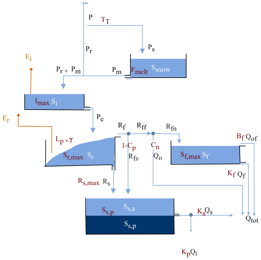
Figure 3 The model structure used to represent the HOAL catchment. Light-blue boxes indicate the hydrologically active, individual storage volumes that contribute to total discharge (Q_tot). The darker-blue box S_s,p indicates a hydrologically “passive” mixing groundwater volume. Blue lines indicate snow and water fluxes, while orange lines indicate water vapour fluxes. Model parameters are shown in red adjacent to the model component they are associated with. All model equations are defined in Table 1, and symbols are defined in Table 2.

Table 1 Water balance and constitutive equations of the hydrological model (Fig. 3). P (mm d⁻¹) is total precipitation, P_s (mm d⁻¹) is solid precipitation (snow), P_r (mm d⁻¹) is liquid precipitation (i.e. rain), P_m (mm d⁻¹) is snowmelt, P_e (mm d⁻¹) is throughfall, E_i (mm d⁻¹) is interception evaporation, E_a (mm d⁻¹) is evaporation from the root zone, R_f (mm d⁻¹) is total preferential fast response, R_fs (mm d⁻¹) is fast recharge to slow-responding reservoir, R_ff (mm d⁻¹) is preferential fast response, Q_o (mm d⁻¹) is infiltration excess overland flow, R_fn (mm d⁻¹) is preferential fast response to the fast-responding bucket, Q_f (mm d⁻¹) is flow from the fast-responding reservoir, Q_of (mm d⁻¹) is saturation excess overland flow from the fast-response bucket, R_s (mm d⁻¹) is slow recharge to the slow-responding reservoir, Q_s (mm d⁻¹) is flow from the slow-responding reservoir, Q_l (mm d⁻¹) is deep infiltration loss, and Q_tot (mm d⁻¹) is the total discharge. A list of model parameters and their definitions is provided in Table 2.

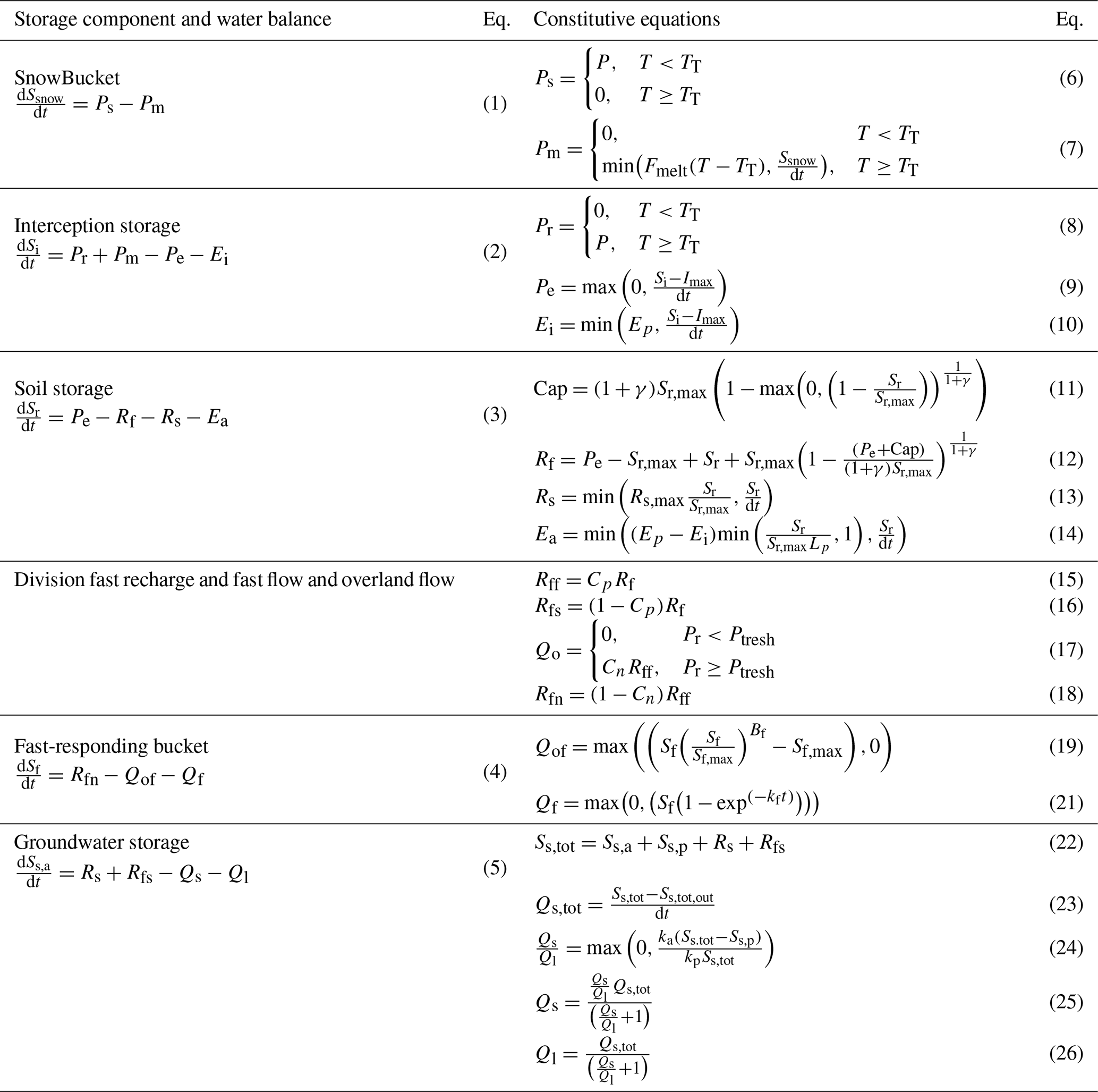
Table 2 Definitions and uniform prior distributions of the parameters of the solute-transport model (Fig. 3).

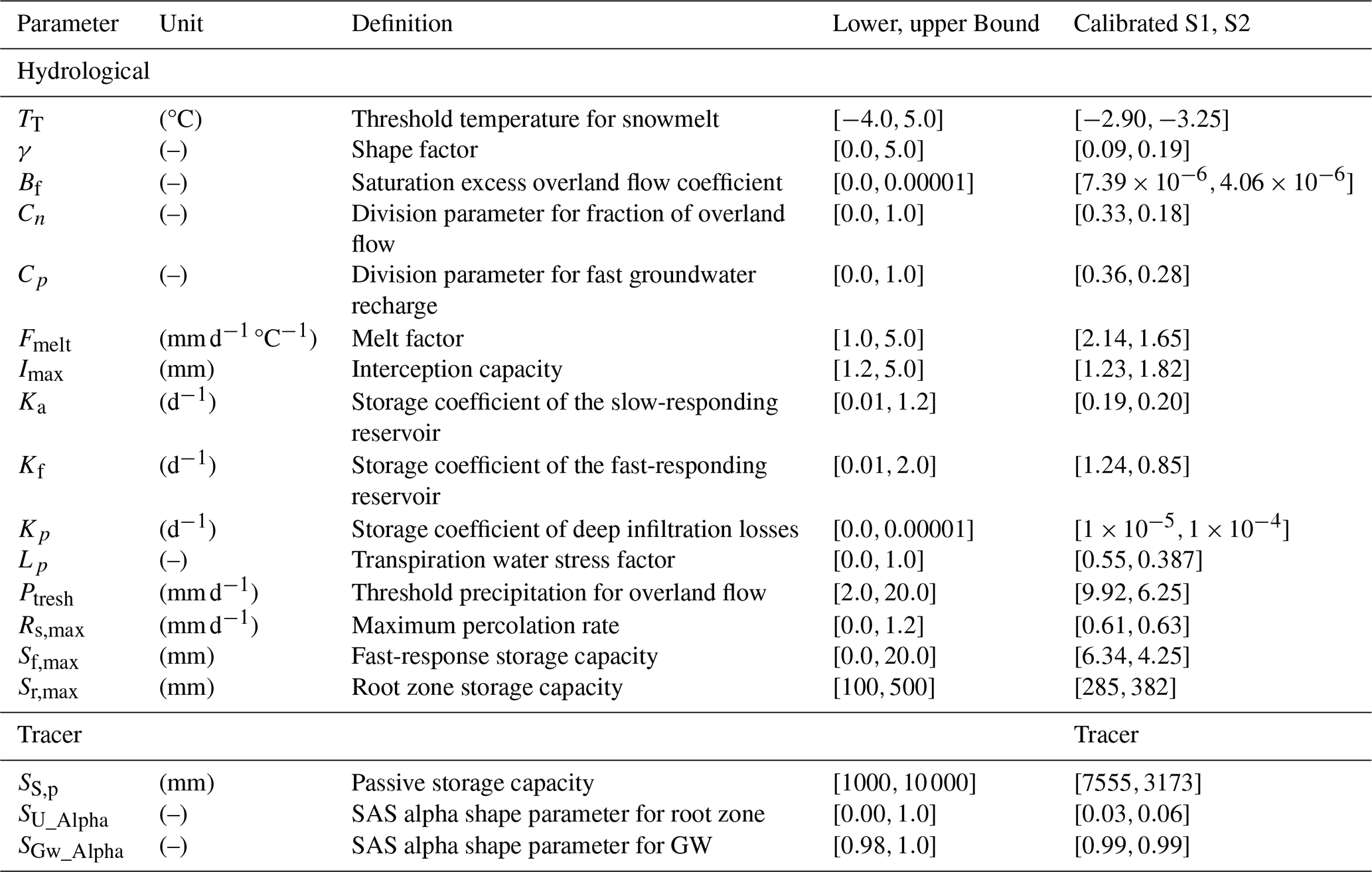
Precipitation P (mm d⁻¹) below the threshold temperature T_T (°C) enters the catchment as snow P_s (mm d⁻¹, Eq. 6) and accumulates in the snow bucket S_snow (mm). Snowmelt P_m (mm d⁻¹) was then computed with the degree-day method (Eq. 7), driven by the melt factor F_melt ($\mathrm{mm}{\mathrm{d}}^{-\mathrm{1}}\mathrm{°}{\mathrm{C}}^{-\mathrm{1}}$) as described by Gao et al. (2017) and Girons Lopez et al. (2020). Rainwater P_r (mm d⁻¹), combined with snowmelt P_m (mm d⁻¹), passes through the canopy interception storage S_i (mm). Water that is not evaporated as interception evaporation E_i (mm d⁻¹, Eq. 10) enters the unsaturated root zone S_r (mm) as throughfall P_e (mm d⁻¹, Eq. 9) based on the water balance of the canopy interception storage (Nijzink et al., 2016) (Eq. 2). Water from the root zone S_r (mm) can be released as (i) fast discharge R_f (mm d⁻¹, Eq. 12), which is based on a critical storage capacity Cap calculated using S_r,max and the shape factor γ (–); (ii) slow recharge to the active groundwater storage S_s,a (mm) through a slower percolation flux R_s (mm d⁻¹, Eq. 13), which is driven by the maximum percolation rate R_s,max (mm d⁻¹); or (iii) the combined flux of root zone transpiration and soil evaporation E_a (mm d⁻¹, Eq. 14) defined by the transpiration water stress factor L_p (–). The fast, preferential discharge R_f (mm d⁻¹) is subsequently divided into several steps to account for fast-flow paths. These are the preferential flow recharging groundwater R_fs (mm d⁻¹, Eq. 15); the infiltration excess overland flow reaching streamflow Q_o (mm d⁻¹, Eq. 16), which is regularly observed in the HOAL catchment (Blöschl et al., 2016); and the lateral subsurface flux R_fn (mm d⁻¹, Eq. 17). Firstly, the fast groundwater recharge R_fs (mm d⁻¹, Eq. 15) is defined by the division parameter (1−C_p). The remaining water R_ff (mm d⁻¹, Eq. 15) is then further divided to account for infiltration excess overland flow Q_o (mm d⁻¹, Eq. 16), which is defined by the division parameter C_n (–) and the threshold parameter P_tresh (mm d⁻¹) (Horton, 1933). We assumed a constant value for the division parameter C_n (–) to limit the number of calibration parameters in the spirit of model parsimony. After the subtraction of fast groundwater recharge and overland flow, the remaining fast and lateral subsurface flux R_fn (mm d⁻¹, Eq. 17) enters the fast storage component S_f (mm, Eq. 4). If the maximum capacity of S_f (mm, Eq. 4) is exceeded, water is released as saturation excess overland flow Q_of (mm d⁻¹, Eq. 18). Otherwise, it is released into the stream as fast flow Q_f (mm d⁻¹, Eq. 19).

Groundwater storage was separated into an “active” groundwater storage S_s,a and a hydrologically “passive” storage volume S_s,p (mm). S_s,p (mm) does not change over time if there are no deep infiltration losses, such that $\mathrm{d}{S}_{\text{s,p}}/\mathrm{d}t=\mathrm{0}$ (Zuber, 1986; Hrachowitz et al., 2016; Wang et al., 2023). This passive storage does not contribute to runoff, but its role is to isotopically mix water of the active storage with water of the passive storage which is represented as $S_{\text{s,tot}}=S_{\text{s,a}}+S_{\text{s,p}}$. The use of the total groundwater storage S_s,tot facilitates contributions from both S_s,a and S_s,p to the age structure of the outflow Q_s (mm d⁻¹, Eq. 24). Water enters the groundwater storage as a sum of slow percolation R_s (mm d⁻¹) and fast recharge R_fs and is released as base flow Q_s (mm d⁻¹, Eq. 24) and deep infiltration losses Q_l (mm d⁻¹, Eq. 25).

2.3 Tracer transport model

2.3.1 Rank StorAge Selection (rSAS) function

We combined the hydrological model, as described in the previous section, with a transport model that utilizes the age rank StorAge Selection (rSAS) function, which ranks stored water volumes by age (Harman, 2015; Benettin et al., 2017) to capture the variability of outflow ages over time. The general theoretical framework of the transport model relies on the studies of Botter et al. (2009), van der Velde et al. (2012), Harman (2015), and Benettin et al. (2015). At any given time t, each storage $S_{T,m,j}\left(t\right)$ defined within the hydrological model (Fig. 2) stores water of different ages. These ages are represented as T and trace back to past precipitation inputs at age T=0. The age distribution of storage at time t is termed p_s(T,t). The outfluxes (e.g. evapotranspiration and discharge) consist of specific age subsets from the storage, resulting in distinct age-ranked distributions for the water leaving the storage. These are termed $p_{E,T}(T,t)$ for evapotranspiration and $p_{Q,T}(T,t)$ for discharge. At each given time t, the total water volume in storage is also characterized by its tracer composition and distributions C_S(T,t), which can be traced back to past precipitation inputs. In the case of an ideal tracer, this is equal to the water stable isotope composition of past precipitation ($P_{\mathit{\delta }{}^{\mathrm{18}}\mathrm{O}}$) upon entering the catchment at time t−T – i.e. C_P(t−T). As a result, output fluxes are characterized by water stable isotope compositions ($Q_{\mathit{\delta }{}^{\mathrm{18}}\mathrm{O}}$, $Q_{\mathit{\delta }{}^{\mathrm{2}}\mathrm{H}}$) and C_Q(t−T) for streamflow and (ET${}_{\mathit{\delta }{}^{\mathrm{18}}\mathrm{O}}$, ET${}_{\mathit{\delta }{}^{\mathrm{2}}\mathrm{H}}$) and C_ET(t−T) for evapotranspiration.

2.3.2 Integration of the rSAS function concept and the hydrological model

The water age balance (Eq. 27) was formulated individually for each of the j storage components of the model such as canopy interception or the root zone based on their transport dynamics. The change in water storage is the difference between age-ranked input volumes $I_{T,j}(T,t)$ (mm d⁻¹) and age-ranked output volumes $O_{T,j}(T,t)$ (mm d⁻¹) (Botter et al., 2011; Harman, 2015; van der Velde et al., 2012).

$$\begin{array}{}\text{(27)}& \begin{array}{rl}{\displaystyle \frac{\partial S_{T,j}(T,t)}{\partial t}}& +{\displaystyle \frac{\partial S_{T,j}(T,t)}{\partial T}}=\\ {\sum }_{n=\mathrm{1}}^N& I_{T,n,j}(T,t)-{\sum }_{m=\mathrm{1}}^M{O}_{T,m,j}(T,t)\end{array}\end{array}$$

$\partial S_{T,j}(T,t)/\partial T$ is the ageing process of water in storage, N and M are the number of inflows and outflows from that storage component (e.g. for the root zone, these would be E_a, R_f, and R_s) (Fig. 3). Each age-ranked outflow $O_{T,m,j}(T,t)$ (Eq. 28) from a specific storage component j (Fig. 3) depends on the outflow volume O_m,j(t) which was estimated by the hydrological balance component of the model (see Sect. 2.2) and the cumulative age distribution $P_{o,m,j}(T,t)$ of that outflow.

$$\begin{array}{}\text{(28)}& O_{T,m,j}(T,t)=O_{m,j}\left(t\right)P_{O,m,j}(T,t)\end{array}$$

The cumulative age distribution $P_{o,m,j}(T,t)$ (Eq. 29), which is the backward transit time distribution (TTD) of that outflow in cumulative form, depends on the age-ranked distribution of water in the storage component j, represented by $S_{T,j}(T,t)$ for time step t and the probability density function, which, in this case, is the SAS function ${\mathit{\omega }}_{o,m,j}$ (or ${\mathrm{\Omega }}_{o,m,j}$ in its cumulative form) of that flux.

$$\begin{array}{}\text{(29)}& P_{O,m,j}(T,t)={\mathrm{\Omega }}_{O,m,j}\left(S_{T,j}\right(T,t),t)\end{array}$$

The SAS function ${\mathit{\omega }}_{o,m,j}$ (or ${\mathrm{\Omega }}_{o,m,j}$ in its cumulative form) is a probability density function of normalized rank storage $S_{T,\text{norm},j}(T,t)$ (Eq. 31) at time t, which can also be formulated as the residence time distribution (RTD) of storage component j (e.g. the root zone) at time t (Eq. 30). Normalizing the age-ranked storage prevents the rescaling of ${\mathit{\omega }}_{o,m,j}$ at each time step to conserve mass balance. Therefore, we used normalized rank storage (Eq. 5) to bind the age-ranked storage to the interval [0,1].

$$\begin{array}{}\text{(30)}& {\displaystyle }{p}_{O,m,j}(T,t)={\stackrel{\mathrm{‾}}{\mathit{\omega }}}_{O,m,j}\left(S_{T,j}\right(T,t),t){\displaystyle \frac{\partial S_{T,j}}{\partial T}}\text{(31)}& {\displaystyle }{S}_{T,\text{norm},j}(T,t)={\displaystyle \frac{S_{T,j}(T,t)}{S_j\left(t\right)}}\end{array}$$

The δ¹⁸O composition, from entering the catchment as precipitation to leaving it as streamflow, was tracked through each individual storage component based on the tracer balance (Eq. 32) (e.g. Harman, 2015; Benettin et al., 2017):

$$\begin{array}{}\text{(32)}& \begin{array}{rl}& C_{O.m,j}\left(t\right)=\\ & {\int }_{\mathrm{0}}^{S_j}{C}_{S,J}\left(S_{T,j}\right(T,t),t){\stackrel{\mathrm{‾}}{\mathit{\omega }}}_{O,m,j}\left(S_{T,j}\right(T,t),t)\mathrm{d}{S}_{\mathrm{T}},\end{array}\end{array}$$

where $C_{o,m,j}$ is the δ¹⁸O composition in outflow m from storage component j at time t, and C_s,j is the δ¹⁸O composition of water in storage at time t.

2.3.3 Time-variable and conditional SAS functions

Previous studies found a difference in transport processes between wet and dry periods (Weiler and McDonnell, 2007; Beven, 2010; Beven and Germann, 2013; Klaus et al., 2013; Loritz et al., 2017; Hrachowitz et al., 2021; Wang et al., 2025). This suggests that SAS functions are time-variable and can be formulated as varying between the preferential release of younger water, the preferential release of older water, or no preference (uniformly selected) (van der Velde et al., 2012, 2015; Hrachowitz et al., 2016).

In this study, we used beta distributions with the shape and scale parameters α (–) and β (–) as SAS functions. When both parameters of the beta distributions are equal to 1 ($\mathit{\alpha }=\mathit{\beta }=\mathrm{1}$), water was uniformly sampled from storage without a preference for specific ages. If α<β (or α>β), a selection preference for younger (or older) water existed. To limit the number of parameters, we kept β equal to 1. The time variability of the SAS function shape was then based on age-ranked storage and the shape parameter (α), which was bounded between [0,1] for the preference of younger storage and was [α>1] for the preference of older storage. In the following, we used this approach for the root zone storage S_r. In contrast, all other storage components (e.g. snow, groundwater) were based on uniform sampling (α=1, β=1). Despite the shape parameters being fixed to uniform sampling in each of these storage components, the resulting overall SAS function, aggregating the individual storage components, was nevertheless time-variable due to the different timescales and the temporally varying contributions of the individual components (Eq. 30).

Previous studies have shown that, as soil moisture increases, preferential flow increasingly bypasses small pore volumes, leading to the release of younger water (Weiler and McDonnell, 2007; Beven, 2010; Loritz et al., 2017; Hrachowitz et al., 2021). To mimic this behaviour, SAS functions for the fast preferential flow R_f (mm d⁻¹) were formulated with a time variable shape factor α(t) (Fig. 4), which varied between 0 and 1 for each time step t. The variation in α(t) was implemented by following Hrachowitz et al. (2013) and van der Velde et al. (2015) by varying it as a function of the stored water volume S_r(t) and the maximum storage capacity (S_r,max), as shown in Eq. (33) and Fig. 4 (scenario 1):

$$\begin{array}{}\text{(33)}& \mathit{\alpha }\left(t\right)=\mathrm{1}-{\displaystyle \frac{S_{\mathrm{r}}\left(t\right)}{S_{\text{r,max}}}}(\mathrm{1}-{\mathit{\alpha }}_{\mathrm{0}}),\end{array}$$

where α₀ is a calibration parameter representing a lower bound between [0,1] so that α(t) can vary between α₀ and 1, and α(t)=1 indicates a uniform sampling SAS function at low soil moisture (dry soil) (Fig. 4a, A). This formulation (scenario 1, Fig. 4a) leads to an increasing preferential release of younger water as the system becomes wetter.

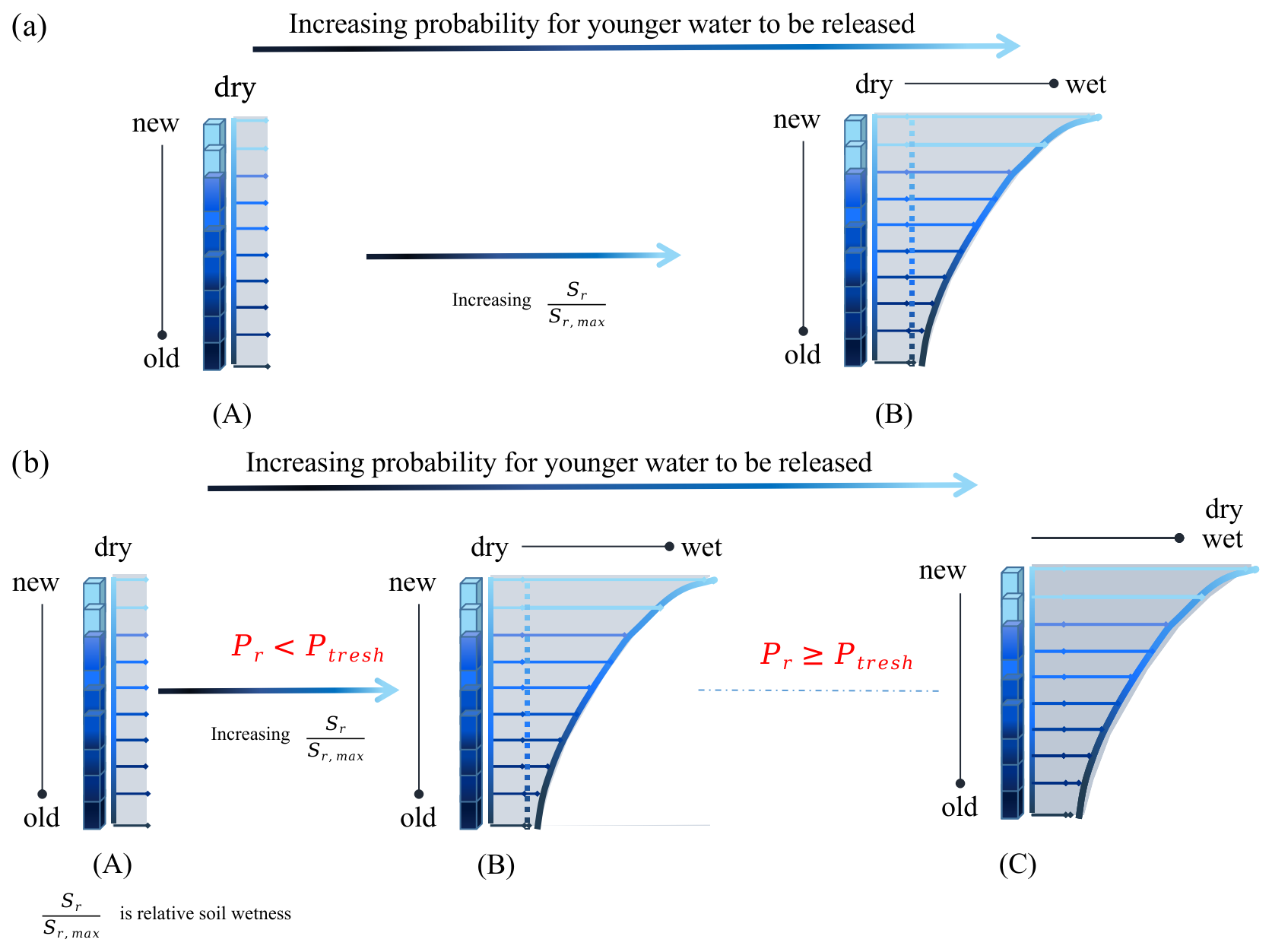
Figure 4 The two tested scenarios for determining the shape of the time-variable SAS function for the fast flux R_f (mm d⁻¹) (Fig. 3). The age-ranked storage probability function is shown as vertical bars in all panels (A, B, and C), with the light-blue colour representing young water (at the top of the vertical bars), while the dark-blue colour represents old water (at the bottom of the vertical bars). (a) In scenario 1, the time-variable SAS function depends on the ratio of the current storage S_r to the maximum storage capacity S_r,max, with the preference for young water increasing as storage increases from A to B (Eq. 33). (b) In scenario 2, the condition (A to B) only applies when the precipitation intensity does not exceed the threshold intensity (P_tresh). If it does exceed P_tresh, young water is preferentially released from storage (panel C), regardless of the current wetness state.

Previous research highlighted the non-linearity of flow processes in the HOAL catchment, where precipitation can quickly generate fast runoff and bypass the soil storage as fast overland or subsurface lateral flow (Blöschl et al., 2016; Exner-Kittridge et al., 2016; Vreugdenhil et al., 2022; Hövel et al., 2024; Szeles et al., 2024). To mimic and test this in our study, SAS functions for the fast preferential flow, R_f (mm d⁻¹), were formulated with a time-variable shape factor α(t), which varies as a function of soil moisture, as in Eq. (33) (scenario 1, Fig. 4a), but additionally becomes equal to α₀ (–) (lower bound) when precipitation intensity P_I (mm d⁻¹) exceeds a certain threshold P_tresh (scenario 2, Fig. 4b, Eq. 34).

$$\begin{array}{}\text{(34)}& \mathit{\alpha }\left(t\right)=\left\{\begin{array}{ll}{\mathit{\alpha }}_{\mathrm{0}},& P_{\mathrm{r}}\left(t\right)\ge P_{\text{tresh}}\\ \mathrm{1}-\frac{S_{\mathrm{r}}\left(t\right)}{S_{\text{r,max}}}(\mathrm{1}-{\mathit{\alpha }}_{\mathrm{0}}),& P_{\mathrm{r}}\left(t\right)<P_{\text{tresh}}\end{array}\right.\end{array}$$

This formulation (scenario 2, Fig. 4) leads to (i) an increasing preferential release of younger water with increasing soil moisture and (ii) a higher probability of releasing younger water that bypasses the soil-stored water when precipitation intensity P_I (mm d⁻¹) exceeds the threshold intensity (P_tresh).

2.4 Model optimization

The model was run with a daily time step for the time period between October 2013 and 30 December 2018 to calibrate the 15 hydrological and 2 tracer transport model parameters (Table 2). We used 1 year of data – from October 2013 to October 2014 – as a warm-up period. Using an objective function that combines six performance criteria (Table 3) related to streamflow and tracer dynamics, we implemented the differential evolution algorithm (Storn and Price, 1997) to optimize model parameters.

Table 3 Signatures for streamflow, the δ¹⁸O signal in streamflow, and the associated performance metrics used for model calibration scenarios and evaluation.

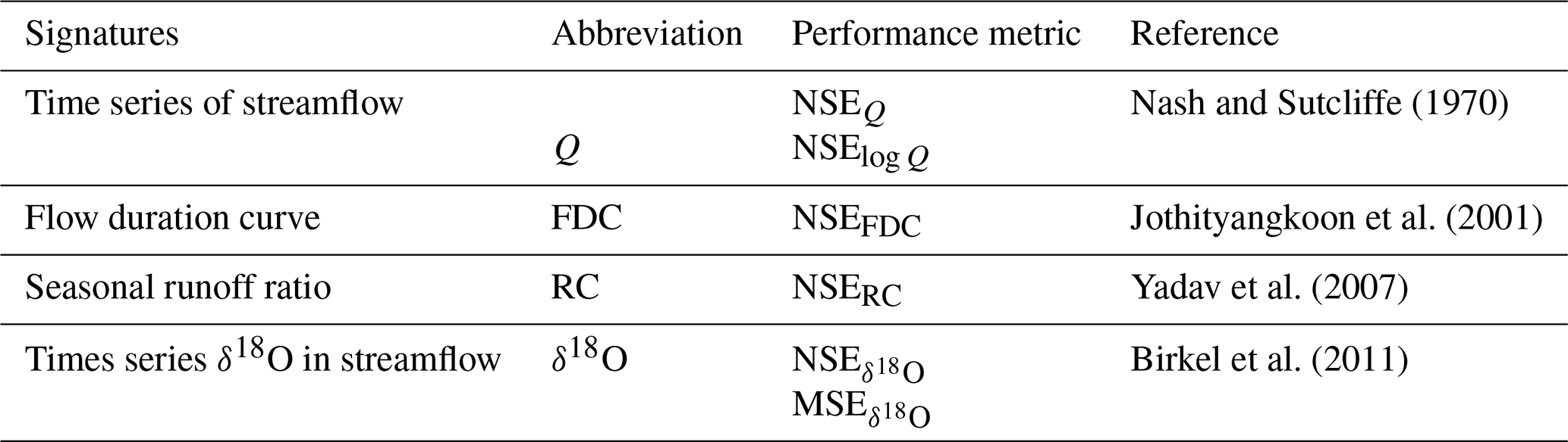
For model calibration and evaluation, we used six performance metrics (Table 3) that describe the model's ability to simultaneously reproduce different signatures associated with streamflow Q (mm d⁻¹) and δ¹⁸O dynamics of the streamflow (Eq. 35). These are the Nash–Sutcliffe efficiencies (NSEs) (Nash and Sutcliffe, 1970) of streamflow, of the logarithmic streamflow, of the flow duration curve, and of the time series of seasonal runoff ratios (averaged over 3 months). For δ¹⁸O signals, we used the NSE of δ¹⁸O of all measured samples (daily event and weekly grab samples) (Fig. 2c) and the mean square error (MSE) of weekly grab samples (Fig. 2d). Similarly to Wang et al. (2024), the individual performance metrics were aggregated into the Euclidean distance D_E to the perfect model using equal weights for the six streamflow signals and the two tracer signatures according to the following:

$$\begin{array}{}\text{(35)}& D_{\mathrm{E}}=\sqrt{{\displaystyle \frac{\mathrm{1}}{\mathrm{2}}}\left({\displaystyle \frac{{\sum }_{i=m}^M(\mathrm{1}-E_{Q,m}{)}^{\mathrm{2}}}{M}}+{\displaystyle \frac{{\sum }_{i=n}^N(\mathrm{1}-E_{\partial {}^{\mathrm{18}}\mathrm{O},n}{)}^{\mathrm{2}}}{N}}\right)},\end{array}$$

where M is the number of performance metrics with respect to streamflow, N is the number of performance metrics for tracers in each combination, and E is the evaluation matrix based on goodness-of-fit criteria. D_E is the Euclidean distance to the perfect model, with zero indicating a perfect fit. We selected the 50 best parameter sets ranked by decreasing Euclidean distance D_E for model evaluation.

We used two scenarios for model calibration, where the formulation for hydrological fluxes was identical, but the transport formulation differed for the lower bound of the SAS function shape α₀ (–), as described in Sect. 2.3.3: scenario 1 (S1), where α(t) represents a linear function of wetness ($S_{\mathrm{r}}/S_{\text{r,max}}$) (Eq. 33), and scenario 2 (S2), with α(t) being a linear function of wetness ($S_{\mathrm{r}}/S_{\text{r,max}}$) if precipitation intensity is less than the threshold intensity P_tresh. However, if precipitation intensity exceeds the threshold intensity (P_tresh), α(t) is set to a strong preference for young-water release, with the shape factor α(t)=α₀ (–) (Eq. 34).

2.5 Model comparison and data analysis

We evaluated the performance of the model under two scenarios using six performance metrics, which are listed in Table 3, for the tracking period from October 2014 to December 2018. Next, we analysed transit times in relation to hydrological and hydroclimatic drivers by categorizing water into different age thresholds. These thresholds included the following: T<2 d and T<7 d, representing “event” water; $\mathrm{7}<T<\mathrm{90}$ d, representing young water with some delay; and $\mathrm{90}<T<\mathrm{365}$ d, representing longer transit times. The streamflow age fraction F_Q (T<T_age days) was calculated based on the sum of TTDs, where T<T_age in days. For example, the age fraction of streamflow, F_Q (T<90 d), was calculated based on the sum of TTDs, where T<90 d.

We calculated the mean and maximum percentage of streamflow fractions for transit times of T<2 d, T<7 d, T<90 d, $\mathrm{7}<T<\mathrm{90}$ d, and $\mathrm{90}<T<\mathrm{365}$ d. We also compared the variation in the mean and maximum percentage of streamflow water age fractions for different seasons, namely autumn (September, October, November), winter (December, January, February), spring (March, April, May), and summer (June, July, August), as well as for distinct wetness states (dry, drying, wet, and wetting periods). Dry days were marked by flows less than the 25th quantile, while wet days were marked by flows higher than the 75th quantile. Drying days marked any decay between the 25th quartile and the 75th quartile, whereas wetting days were marked as any increase between the 25th quartile and the 75th quartile.

Furthermore, we compared the relationship between transit times and hydrological and hydroclimatic drivers, specifically streamflow Q (mm d⁻¹), precipitation intensity P_I (mm d⁻¹), and volumetric soil water content (SWC) (%) for the tracking period, as well as across different seasons and wetness states, to understand variations in the control mechanisms. This analysis was conducted by comparing Spearman rank correlation coefficients of water age fractions with the hydroclimatic drivers.

3 Results

3.1 Model calibration

The model parameters selected for the HOAL catchment during the calibration period from October 2014 to December 2018 reproduced the general features of the hydrograph (Fig. 5). The best-performing model generally captured both the timing and magnitude of high- and low-flow events, independent of the selected scenario (NSE_Q=0.61 for both scenarios, Fig. 5a), with the exception of overestimations of low flows during summer 2016 and underestimation of low flows during winter 2017. The 3-month averaged runoff ratio (RC) was reproduced, with NSE values of 0.89 for scenario 1 and 0.83 for scenario 2 (Fig. 5b and e). The flow duration curve (FDC) was also reproduced, with a Nash–Sutcliffe efficiency (NSE_FDC) of 0.51 for scenario 1 and 0.50 for scenario 2 (Fig. 5d and e). Additionally, low flows were reproduced, with a median Nash–Sutcliffe efficiency of log flows (NSE_log Q) of 0.65 (Fig. 5c and e). For several rain storms, the model reproduced the sharp δ¹⁸O fluctuations during events and a highly stable δ¹⁸O signal between consecutive events (Fig. 5c) for both scenarios. However, indeed, scenario 2 showed considerable improvements for the very negative winter δ¹⁸O stream values in 2015 and 2018, as well as for several events in the summer of 2016, 2017, and 2018. The performance metrics based on median δ¹⁸O signals were higher for scenario 2, with, for example, an NSE${}_{\mathit{\delta }{}^{\mathrm{18}}\mathrm{O}}=\mathrm{0.51}$, and then for scenario 1, with an NSE${}_{\mathit{\delta }{}^{\mathrm{18}}\mathrm{O}}=\mathrm{0.31}$ (Fig. 5e). Overall, the Euclidian distance D_E for the 50 best-performing parameter sets decreased from 0.55 to 0.42 for scenario 1 and decreased from 0.57 to 0.37 for scenario 2, showing that scenario 2 generally performed better than scenario 1. For both scenarios, the MSE values for weekly samples (MSE${}_{\mathit{\delta }{}^{\mathrm{18}}\mathrm{O}}$) were comparable (Fig. 5e).

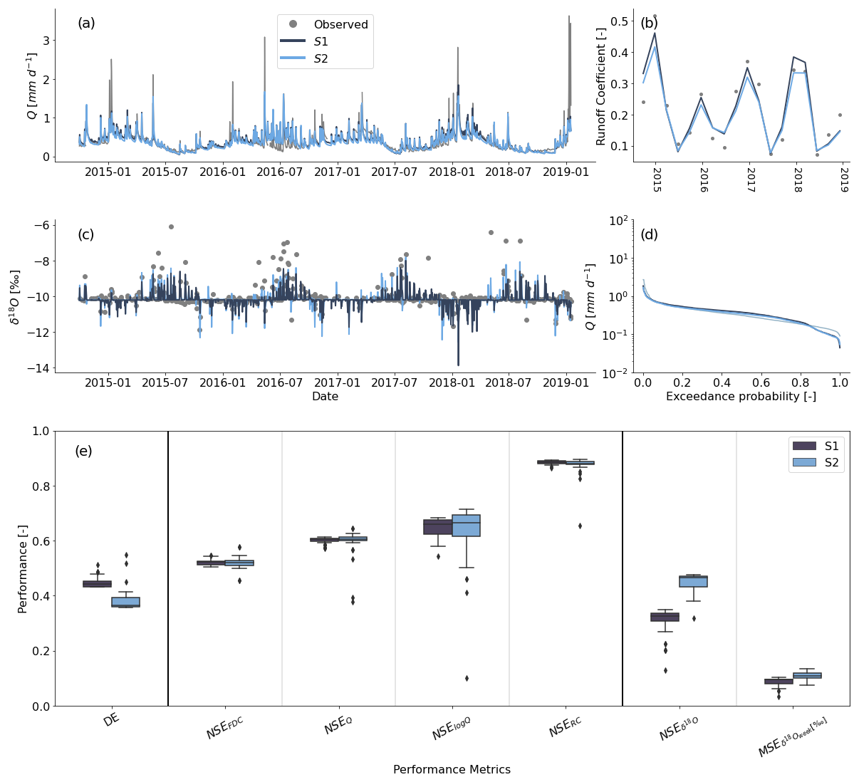
Figure 5 Model calibration results for scenario 1 (S1, dark blue) and scenario 2 (S2, light blue). (a–d) The observed values are shown as grey dots and lines. (a) Streamflow (mm d⁻¹), (b) streamflow's ¹⁸O (‰), (c) the 3-month average runoff coefficient RC (–), (d) the flow duration curve (mm d⁻¹), and (e) boxplots of performance metrics of the two scenarios based on the 50 best-performing parameter sets.

Simulated δ¹⁸O from preferential flow (R_f) is shown in Fig. 6. In scenario 1, where the SAS function for preferential flow is exclusively controlled by soil moisture, the simulated δ¹⁸O signal in stream water was noticeably more dampened compared to scenario 2. This reflects a higher probability of mobilizing older stored water, reducing the direct transmission of event water to the stream. In contrast, scenario 2, which incorporated both soil moisture and precipitation intensity, resulted in a modelled stream water δ¹⁸O signal that more closely resembled both the observed stream water δ¹⁸O and the precipitation input signal. This highlights that accounting for precipitation intensity allows the model to better capture dynamic preferential-flow responses, with a higher probability of mobilizing younger event water into the stream.

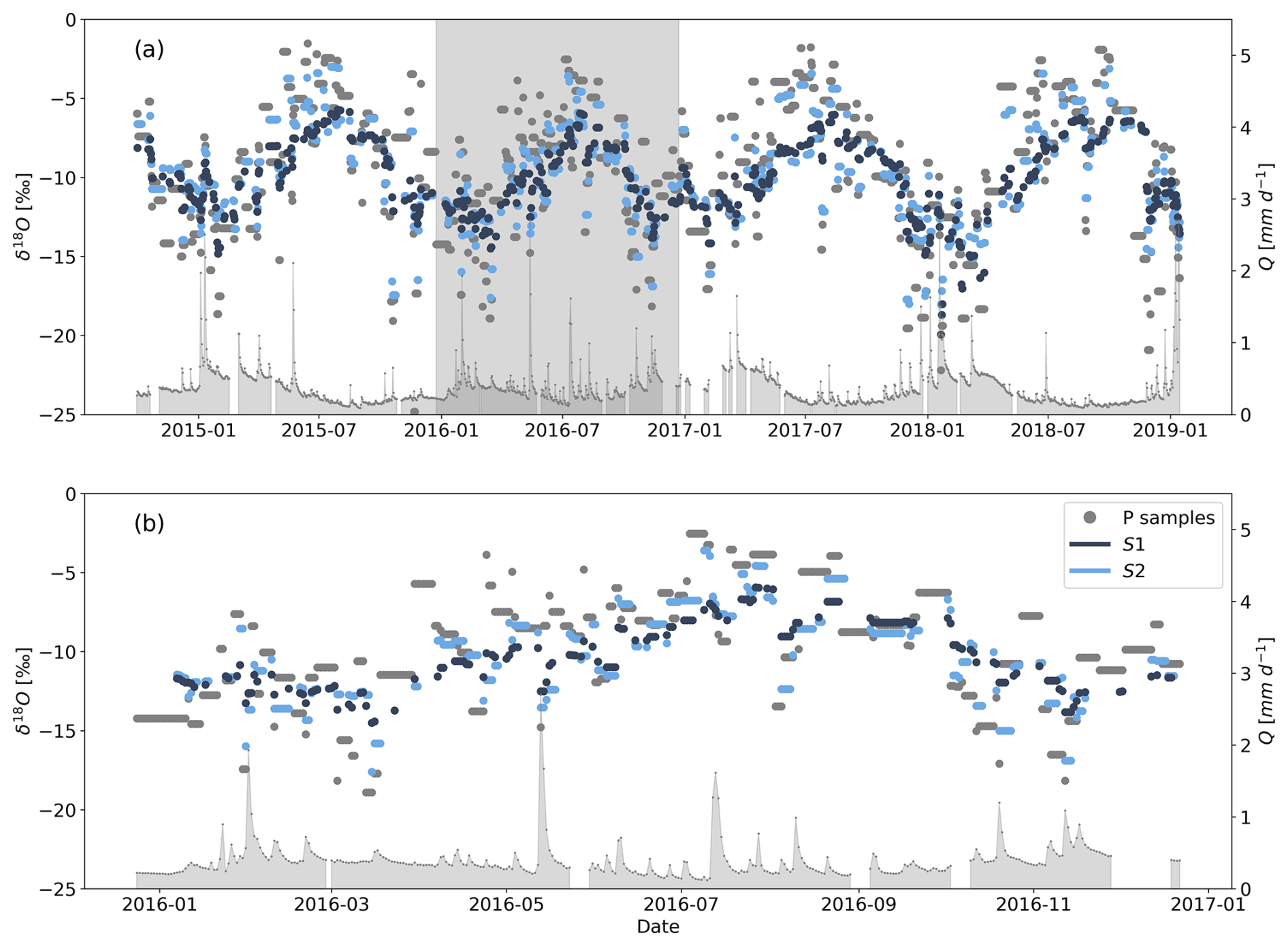
Figure 6 δ¹⁸O simulations of preferential flow (R_f, Fig. 3) resulting from two scenarios. (a, b) The grey-shaded area shows the measured streamflow (Q, mm d⁻¹). (b) Zoom-in of the δ¹⁸O simulations of preferential flow (R_f, Fig. 3) under two scenarios for the year 2016.

3.2 Water transit times and residence times

By tracking the δ¹⁸O signals through the model, we estimated TTDs in streamflow and compared these distributions for different age thresholds, namely T<2 d, T<7 d, $\mathrm{7}<T<\mathrm{90}$ d, T<90 d, and $\mathrm{90}<T<\mathrm{365}$ d (see Sect. 2.4). It is important to acknowledge that the transit time results are inherently tied to the assumptions made and the uncertainties within the modelling process.

Model calibration based on scenario 2 resulted in more young water bypassing storage, as evidenced by the mean percentage of streamflow age fractions younger than 2 d F_Q (T<2 d) and 7 d F_Q (T<7 d) being lower for scenario 1 (2, 27 % and 2.87 %, respectively) compared to for scenario 2 (3.78 % and 4.03 %, respectively) (see Table 4, Figs. 7a and S2 in the Supplement). This was also reflected in individual TTDs for fast preferential flow R_f (mm d⁻¹) (Fig. 3), where, on average, 40 % of fast preferential flow was from recent rainfall (age=1 d) based on scenario 2 compared to 30 % for scenario 1 (Fig. 7e). However, the fraction of streamflow that is younger than 90 d, F_Q (T<90 d) was similar for both scenarios, where the mean percentage for scenario 1 was 6.03 %, while for scenario2 it was 6.53 % (see Table 4 and Fig. 7b).

Table 4 Summary of the mean and maximum (max) percentage of water transit times categorized as T<90, $\mathrm{0}<T<\mathrm{2}$, $\mathrm{0}<T<\mathrm{7}$, $\mathrm{7}<T<\mathrm{90}$, and $\mathrm{90}<T<\mathrm{365}$ in days based on scenario 1 (S1) and scenario 2 (S2).

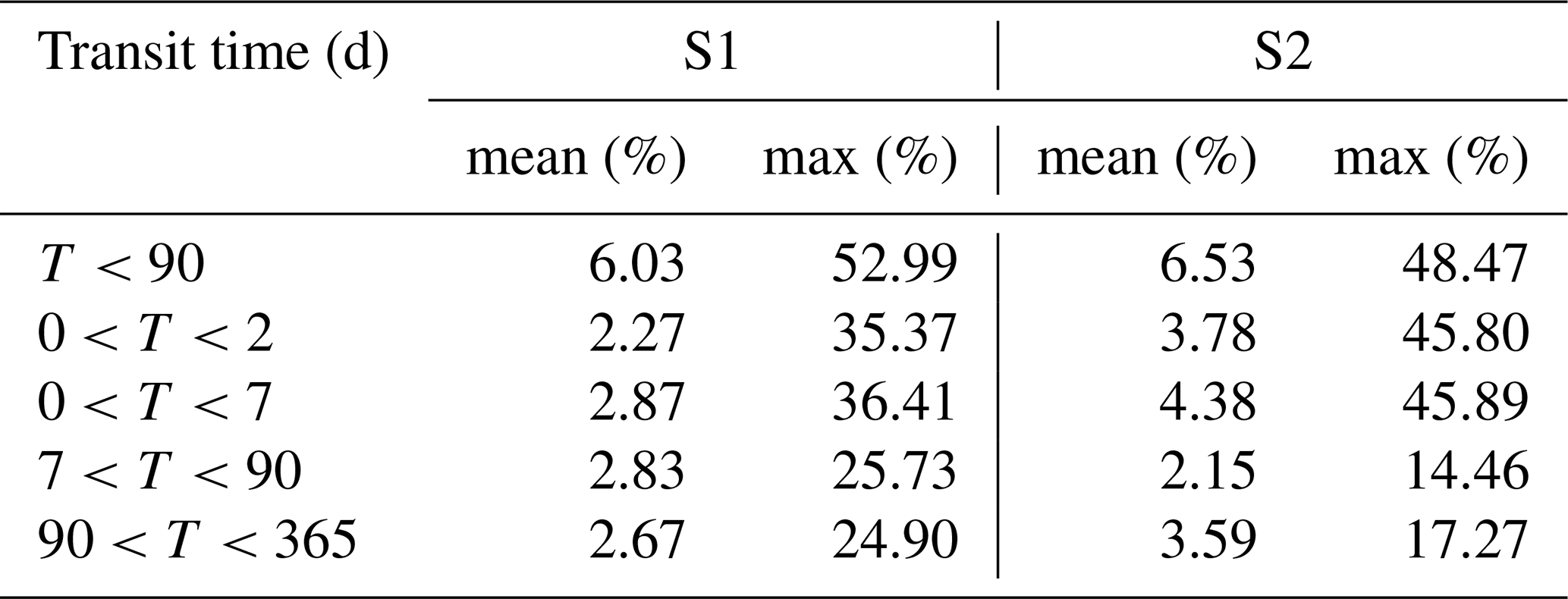
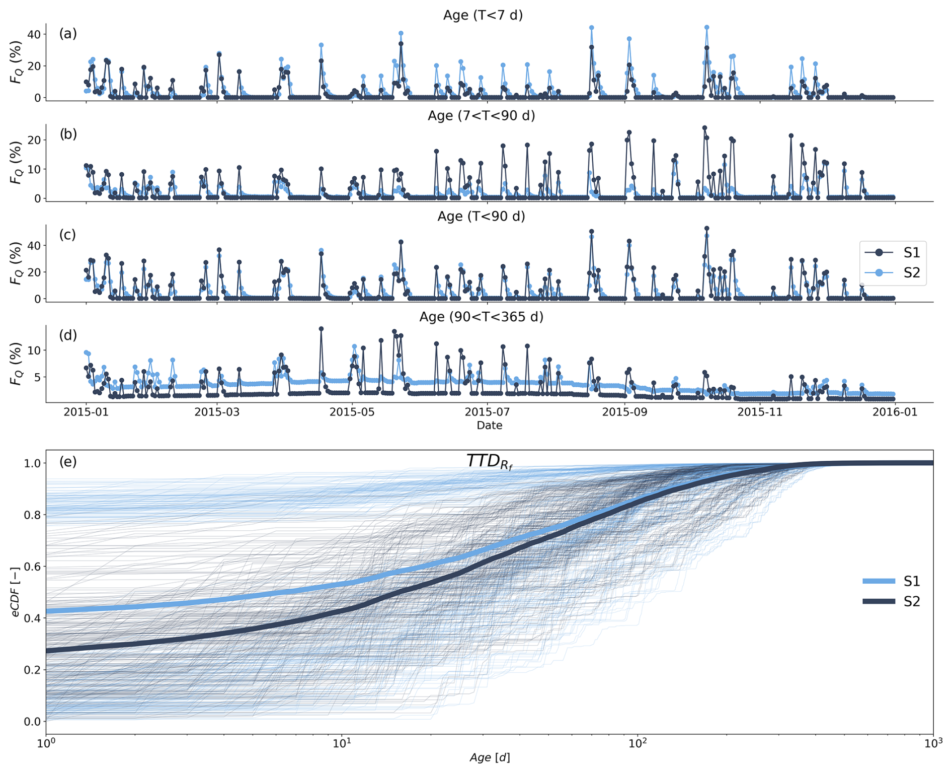
Figure 7 The percentage of water age fractions based on two scenarios for the year 2015. The results for the full calibration period are provided in Fig. S2. (a–e) Dark-blue dots represent the results from scenario 1 (S1), and light-blue dots represent the results from scenario 2 (S2). The age fraction of streamflow was categorized by age: (a) T<7 d, (b) $\mathrm{7}<T<\mathrm{90}$ d, (c) T<90 d, and (d) $\mathrm{90}<T<\mathrm{365}$ d. Panel (e) shows individual transit time distributions (TTDs) based on scenario 1 and scenario 2 for total fast preferential flow R_f (Fig. 3) as empirical cumulative distribution functions (eCDFs) (–). The bold lines in panel (e) show the mean of individual TTDs in cumulative form based on scenario 1 (dark-blue line) and scenario 2 (light-blue line).

3.3 Influence of hydrological and hydroclimatic variables on water age fractions

The influence of hydrological and hydroclimatic variables on water age fractions ($\mathrm{0}<T<\mathrm{7}$, T<90, $\mathrm{90}<T<\mathrm{365}$ in days) was compared by means of Spearman rank correlation coefficients (r, p). Only the precipitation intensity P_I (mm d⁻¹) was strongly correlated with the streamflow water age fraction younger than 7 d (F_Q (T<7 d)) for both scenarios, with a slightly higher correlation coefficient for scenario 1 (S1, r=0.67, p<0.05) compared to scenario 2 (S2, r=0.53, p<0.05) (Fig. 8b). Similarly, water age fractions younger than 90 d (F_Q (T<90 d)) were more correlated with precipitation intensity P_I (mm d⁻¹) than with volumetric soil water content (SWC) (%) or streamflow Q (mm d⁻¹) (Fig. 8d–f). The correlation coefficients (r and p) for P_I (mm d⁻¹) were r=0.71 and p<0.05 for scenario 1 and r=0.62 and p<0.05 for scenario 2. For streamflow age fractions between 90 and 365 d (F_Q ($\mathrm{90}<T<\mathrm{365}$ d)), only scenario 1 resulted in strong correlation coefficients for P_I (mm d⁻¹) (r=0.58, p<0.05) (Fig. 8h). No strong correlations were found for all of the other combinations of the water age fractions in relation to Q (mm d⁻¹) or SWC (%) (Fig. 8).

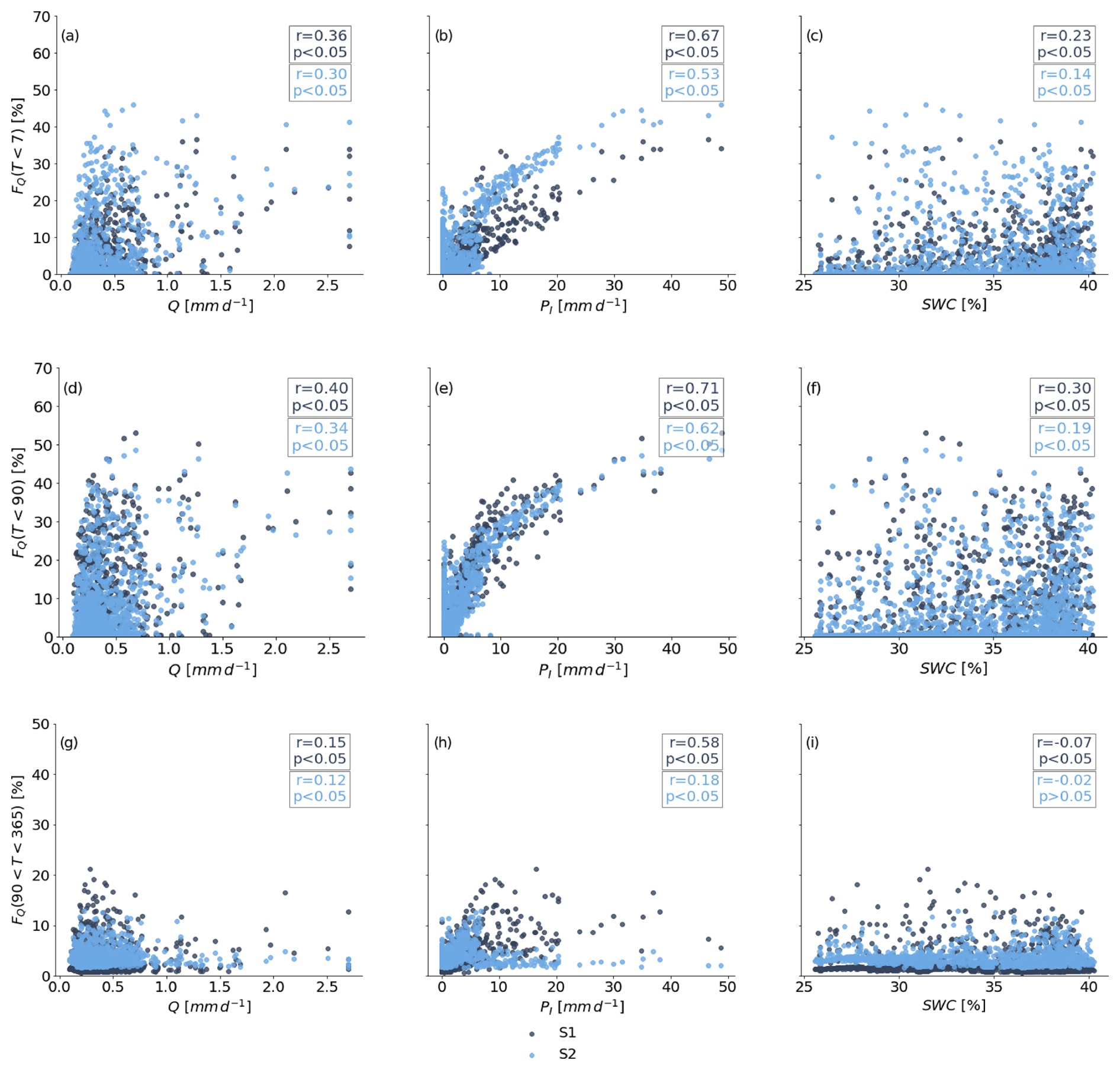
Figure 8 Spearman rank correlation of streamflow water age fractions with the hydrological and hydroclimatic variables: discharge Q (mm d⁻¹), precipitation intensity P_I (mm d⁻¹), and volumetric soil water content (SWC) (%). Panels (a–c) show the correlations of streamflow age fractions younger than 7 d (F_Q (T<7 d)), panels (d–f) show the correlations of streamflow age fractions younger than 90 d (F_Q (T<90 d)), and panels (g–i) show correlations of streamflow age fractions older than 90 d but younger than 365 d (F_Q ($\mathrm{90}<T<\mathrm{365}$ d)) in relation to discharge Q (mm d⁻¹), precipitation intensity P_I (mm d⁻¹), and volumetric water content (SWC) (%).

3.4 Linking water age fractions to hydrological and hydroclimatic drivers in different seasons

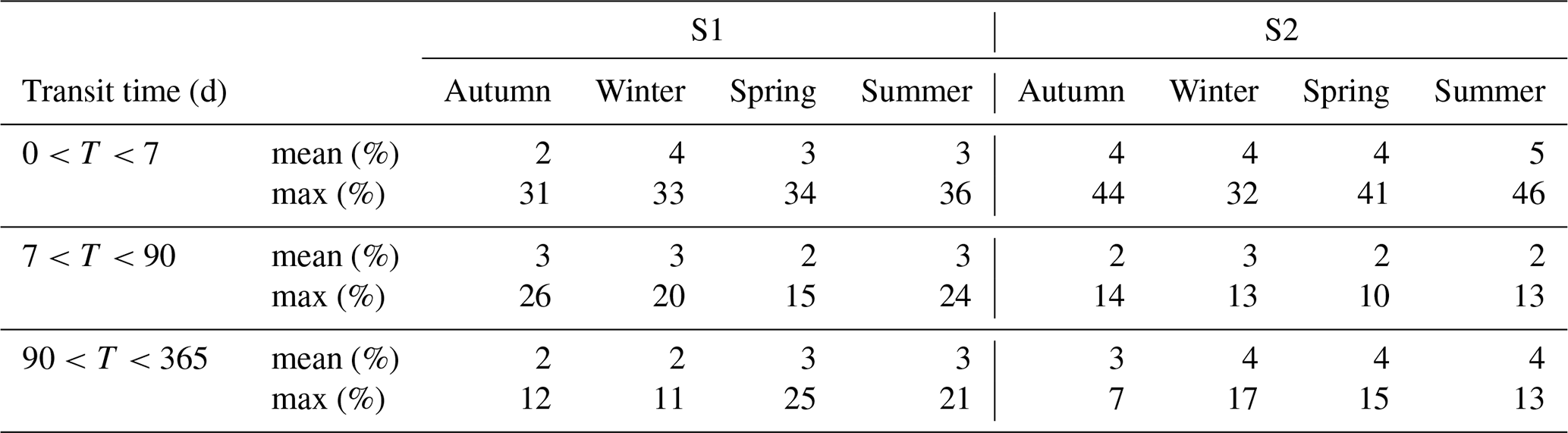
Scenario 2 resulted in a higher fraction of streamflow water younger than 7 d (F_Q (T<7 d)), especially during autumn and summer, compared to scenario 1 (Figs. 9a and 10a). However, during spring and winter, both scenarios reproduced similar results for F_Q (T<7 d). On average, 2 % and 4 % of autumn streamflow was younger than 7 d based on scenario 1 and scenario 2, respectively. For individual events, these values reached up to a maximum of 31 % and 44 % based on scenario 1 and scenario 2, respectively (Table 5). Similarly, in the summer season, scenario 2 resulted in a higher fraction of streamflow younger than 7 d, with an average of 4.48 %, compared to scenario 1 (3 %). For water ages $\mathrm{7}<T<\mathrm{90}$ d and $\mathrm{90}<T<\mathrm{365}$ d, scenario 1 resulted in higher streamflow fractions across all seasons compared to scenario 2 (Fig. 10b and c; Table 5)

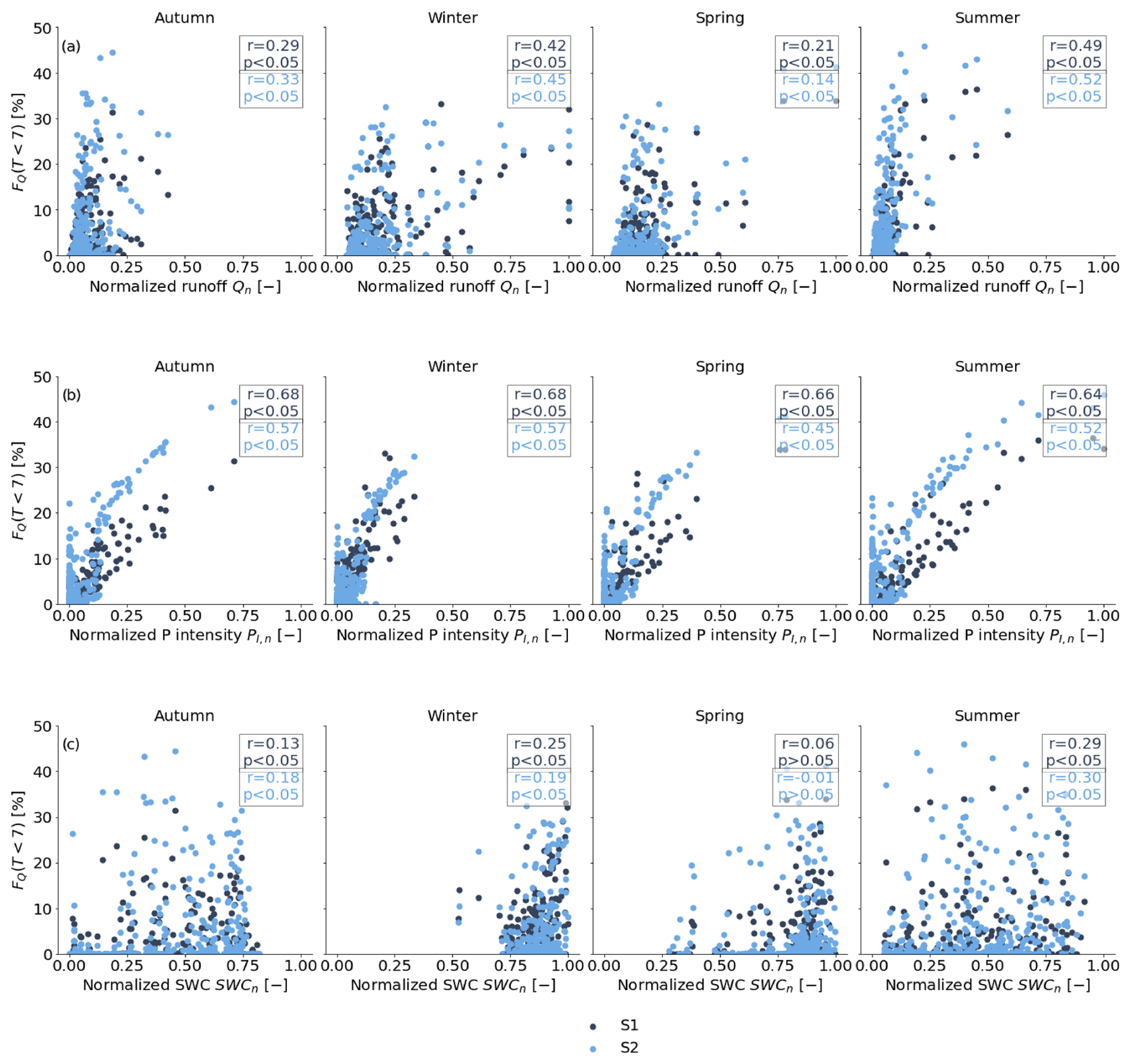
Figure 9 Spearman rank correlation of streamflow water age fractions younger than F_Q (T<7 d) with hydrological and hydroclimatic variables across different seasons (autumn, winter, spring, summer). (a) Normalized discharge Q (–) correlated with F_Q (T<7 d), (b) normalized precipitation intensity P_I,n (–) correlated with F_Q (T<7 d), and (c) normalized volumetric water content (SWC) (–) correlated with F_Q (T<7 d).

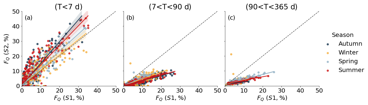
Figure 10 Comparison of estimated water ages based on two scenarios. Streamflow age fraction results from scenario 1 are represented on the x axis, while results from scenario 2 are represented on the y axis. The dashed black lines represent the 1:1 line for all panels. (a) The comparison of estimated water age fractions younger than 7 d, (b) age fractions from 7 to 90 d, and (c) age fractions between 90 to 365 d. The colours indicate different seasons: dark blue represents autumn, yellow represents winter, light blue represents spring, and red represents summer.

Table 5 Summary of the mean and maximum (max) percentage of water transit times categorized by ages of $\mathrm{0}<T<\mathrm{7}$, $\mathrm{7}<T<\mathrm{90}$, and $\mathrm{90}<T<\mathrm{365}$ in days based on scenario 1 (S1) and scenario 2 (S2) for autumn, winter, spring, and summer.

4 Discussion

4.1 Soil moisture is not the only control of transit times

Previous studies have shown that soil moisture plays a significant role in catchment transit times in humid areas, such as the Wüstebach in Germany and the Bruntland Burn catchment in Scotland (Benettin et al., 2017; Hrachowitz et al., 2021). However, in the HOAL catchment of this study, rainfall intensity, beyond soil moisture, was required to account for the complexity of the hydrological and transport response.

For both scenarios (scenario 1: SAS function with soil moisture only; scenario 2: SAS function with soil moisture and rainfall intensity), the mean fraction of relatively short travel times in stream water (T<7, $\mathrm{7}<T<\mathrm{90}$, and T<90 d) was positively correlated with modelled soil moisture (Table S1 in the Supplement). This suggests that catchment soil moisture plays a role in young-water release in the HOAL catchment, which is further supported by the reasonably good simulation results regarding stable isotopes of water when only using soil moisture in the SAS function (NSE=0.31). Therefore, the results correspond well to earlier research, where increasing catchment wetness resulted in younger water reaching the stream (Weiler and Naef, 2003; Zehe et al., 2006; Hrachowitz et al., 2013; Remondi et al., 2018; Rodriguez et al., 2018; Sprenger et al., 2019).

Despite the selection of the SAS function being based exclusively on catchment wetness being adequate for the HOAL catchment, the highly complex runoff generation mechanisms (Blöschl et al., 2016) with a quick-runoff response, particularly during autumn and summer months, highlighted the need for an additional control on the SAS function shape (Figs. 5c and 7a). Indeed, the model performance was better (Fig. 5e) when including precipitation intensities in the SAS function (Fig. 4b). This indicates that the direct contribution of precipitation to streamflow during storm events with high precipitation intensities is important in the HOAL catchment. This behaviour can be explained by several factors that promote fast runoff that bypasses resident water.

The incorporation of both soil moisture and precipitation intensity in the SAS function accounts for the non-linearity of flow processes, mimicking not only the behaviour of saturation excess overland flow but also that of infiltration excess flow and other subsurface fast-runoff flow processes that bypass flow with minimal interaction with resident water (e.g. tile drain flow). The non-linearity of flow processes in the HOAL catchment has been demonstrated through hydrometric analysis and visual observations, which have highlighted the potential controls of soil moisture and event precipitation on runoff (Blöschl et al., 2016; Exner-Kittridge et al., 2016; Vreugdenhil et al., 2022; Hovel et al., 2024; Szeles et al., 2024). Similarly, Vreugdenhil et al. (2022) showed that rainfall and soil moisture are significant and highly non-linear controls on overland flow and tile drainage flow in different parts of the HOAL. For instance, tile drainage in wetlands was more linearly related to soil moisture, whereas, at the hillslope scale, it was more related to precipitation even under low-intensity rainfall. Therefore, it is plausible to assume that, in the HOAL catchment, overland flow exhibits a threshold behaviour related to fast-runoff generation occurring even under low-intensity rainfall.

Additionally, the HOAL catchment consists of a diverse range of soil types, with a high clay content between 20 % and 30 % (Blöschl et al., 2016). Different types of soils may introduce complexities due to surface and subsurface heterogeneity in soil hydraulic conductivity, which significantly influences the shapes of SAS functions (Danesh-Yazdi et al., 2018). Indeed, as previously discussed by Danesh-Yazdi et al. (2018), subsurface heterogeneity in hydraulic conductivity imposes significant variation on the shape of the SAS function, and hydraulic conductivity in HOAL was found to be variable over 2 orders of magnitude, from as low as 1 mm h⁻¹ to as high as 130 mm h⁻¹ (Picciafuoco et al., 2019). Therefore, assuming a smooth functional form for the SAS function in heterogeneous systems may oversimplify its intrinsic variability concerning water age or age-ranked storage. This may also explain why incorporating soil moisture and precipitation intensity, as we did in scenario 2, resulted in better model performance in the simulation of the δ¹⁸O signal in streamflow.

Besides this, the tile drainage system, which covers only 15 % of the catchment (Fig. 1), appeared to play an important role in fast-flow generation. The close resemblance of the δ¹⁸O signal in the tile drainage system in relation to the precipitation δ¹⁸O signal (Fig. 2e and f) provides evidence that some event precipitation contributes to the stream through the tile drain not only in winter but also in summer. A possible explanation for this process in summer months is that larger cracks in the clayey soils, which are directly connected to the tile drainage system, allow for preferential flow that is more dependent on precipitation intensity than on soil moisture. This corresponds with observations from Exner-Kittridge et al. (2016), who noted that, in the HOAL catchment, macropore flow is observed in summer when the topsoil dries and forms cracks due to the high clay content. This emphasizes the critical role of soil texture and structure in influencing water movement during rainfall events.

4.2 Synthesis of streamflow generation processes in the HOAL catchment

The HOAL catchment exhibits a diverse and rapid hydrological response to precipitation events (Blöschl et al., 2016; Exner-Kittridge et al., 2016; Vreugdenhil et al., 2022). This is also evidenced by the on–off response of streamflow and the sharp transition between high-resolution event δ¹⁸O signals and highly stable weekly δ¹⁸O signals observed in the stream (Fig. 2c, e, and f). Tracer compositions measured at weekly intervals remained stable throughout the year (Fig. 2d). However, event-based samples and tile drainage samples showed similar δ¹⁸O patterns compared to precipitation (Fig. 2f), indicating a sharp transition between fast-flow processes and more stable groundwater flow. For several rain storms, the model reproduced the sharp fluctuations during events and a stable δ¹⁸O signal between consecutive events (Fig. 5c) for both scenarios. Nevertheless, the model calibration based on scenario 2 enhanced the model's sensitivity to the timescale of fast flow (Fig. 7a), further emphasizing the critical role of precipitation intensity in influencing hydrological responses in the catchment. In particular, infiltration excess overland flow and precipitation-driven subsurface fast flow were identified as key flow processes, corroborating studies by Blöschl et al. (2016), Széles et al. (2020), and Silasari et al. (2017), who noted that both saturation excess and infiltration excess overland flow typically occur in valley bottoms during prolonged or intensive rainfall, with part of the event water entering the stream as overland flow. The hydrological behaviour of the HOAL catchment supports earlier findings by Kirchner et al. (2023), who noted that a rapid hydrological response often indicates that rainwater moves quickly to channels via overland flow or fast subsurface pathways.

4.3 Catchment transit times

Transit time results indicated that event peaks were primarily a mixture of new precipitation water (T<2 d) and water less than 7 d old that had been stored in the catchment. During events, the fraction of streamflow water for ages of T<7 d, $\mathrm{7}<T<\mathrm{90}$ d, and $\mathrm{90}<T<\mathrm{365}$ d increased for both scenarios (Fig. 7a). However, on average, only ∼4 % of the water was younger than 7 d, and ∼7 % was younger than 90 d (Table 4). This aligns with the findings of previous studies that have shown the majority of water contributing to streamflow to be old, a phenomenon that has been termed the “old-water paradox” (Kirchner, 2003; McDonnell et al., 2010).

Nevertheless, the fraction of stream water younger than 7 d increased from 1 % to up to 45 % on an event scale depending on storm size (Figs. 8b and 9e). This indicated that most precipitation did not mobilize old water in the first place; instead, it drained directly into river networks and contributed to the stream via fast-flow paths. This reflects results reported by Szeles et al. (2024), where their findings showed that the new-water contribution averaged around 50 % during peak flows in selected large events in the HOAL catchment.

Given that the slope of the catchment is relatively low (8 %), another reason can be the high proportion of agriculturally used land, which tends to develop a compacted or sealed surface layer, thus inhibiting or reducing infiltration during heavy rainfall events. Agricultural soils, particularly those with intensive tillage or limited vegetative cover, are prone to surface sealing (Laloy and Bielders, 2010) during heavy rainfall events (e.g a reduction in infiltration capacity as a result of the use of heavy machinery and soil erosion processes. The impact of raindrops can break down soil aggregates at the surface, leading to the formation of a thin, compacted soil layer (i.e. a “soil crust”) that reduces infiltration capacity (Blöschl, 2022). This crust formation can be more pronounced in soils with higher silt content or weak aggregate stability, thereby favouring overland flow and quick-runoff generation during heavy precipitation.

4.4 Catchment transit time variability with hydrological and hydroclimatic conditions

The fraction of stream water younger than 7 d (F_Q (T<7 d)) was positively correlated with precipitation intensities (Fig. 8b), implying that the volume of event water transmitted to streamflow increases with storm size. Similar results were noted by Szeles et al. (2024), who used hydrograph separation methods and highlighted that new-water fractions during events increased with precipitation intensity in the HOAL catchment.

In contrast, the measured volumetric soil water content (SWC) (%) did not strongly correlate with shorter transit times (F_Q (T<7 d) and F_Q (T<90 d)) for either scenario (Fig. 8c and f). This may seem contradictory, but it is plausible to assume that the effect of frequent fast flow in the HOAL catchment dominates and masks the underlying relationship between catchment wetness and transit times. Hövel et al. (2023) found that measured volumetric soil water content was weakly or not at all correlated with event runoff responses, reinforcing the fact that precipitation intensity rather than catchment wetness can be the dominant driver of fast-runoff generation.

Stream water fractions with transit times of less than 90 d (F_Q (T<90 d)) were weakly correlated with discharge Q (mm d⁻¹) (r=0.40 for scenario 1 and 0.34 for scenario 2) but were strongly positively correlated with precipitation intensity P_I (mm d⁻¹) (r=0.71 for scenario 1 and 0.62 for scenario 2) (Fig. 9d and e). These findings support the earlier study by von Freyberg et al. (2018a), who noted that low discharge sensitivity to high fractions of young water can indicate the dominance of fast-runoff flow paths in the hydrological response. This behaviour persists regardless of the magnitude of precipitation events (von Freyberg et al., 2018b), particularly under conditions where the landscape promotes rapid water movement, such as in catchments with certain soil types or topographic features (such as the HOAL catchment). Such behaviour also points to well-developed subsurface flow paths (e.g. tile drains at the hillslope scale) that directly transport water and solutes to the stream, highlighting the catchment's sensitivity to precipitation input.

4.5 Implications and limitations

Being conditional on the assumptions made throughout the modelling process and notwithstanding potential uncertainties, high-frequency water stable isotope data and model calibrations provide relatively strong evidence to support the key findings of this study: both soil moisture and precipitation intensity significantly influence hydrological responses and transit times in the HOAL catchment. This reflects non-linear flow behaviour and a shift towards younger water ages in the stream, particularly during autumn and summer. Soil-wetness-dependent and precipitation-intensity-conditional SAS functions may, therefore, be necessary to better capture and identify the mechanisms driving rapid streamflow generation and their associated timescales, notably in catchments where preferential flows and overland flow are the dominant flow processes. The SAS functions based on both soil moisture and precipitation intensity resulted in an increased probability of rapid mobilization of young water, which is critical for stream water quality and groundwater recharge.

Although, here, the analysis is limited to a small, agricultural catchment with a flashy response, it is plausible to assume that the approach is also, similarly, valid in other settings with diverse hydrological characteristics and where rainfall intensity exceeds infiltration rates, leading to surface runoff or subsurface preferential pathways. By focusing on how soil moisture and precipitation intensity jointly influence younger-water release, the insights of this study can help to develop water management strategies in, for example, agricultural catchments. Managers could better schedule fertilizer applications to minimize nutrient leaching and to reduce water quality deterioration.

There are some limitations in this study that need to be addressed and tested in future research. The model calibration based on both scenarios overestimated low flows during the summer of 2016, despite relatively higher precipitation during that year. This overestimation is likely to be linked to groundwater recharge processes being more complex than represented in the model structure. The overestimation of low flows began after an intense rainfall event (P>50 mm d⁻¹, Fig. 2) followed by several moderate-intensity events. A potential explanation is the activation of flow paths down to the depth of the tile drainage system or the dominant subsurface lateral flow, which may have diverted water directly to the stream, bypassing groundwater infiltration and promoting interflow. Another possibility is the presence of a low-permeability unsaturated transition zone between the root zone and the groundwater table, which may have delayed groundwater recharge. This could also explain why low flows in the winter and spring of 2017 were conversely underestimated. To fully evaluate these hypotheses and to better estimate the recharge processes, additional field observations and more detailed studies focusing on subsurface dynamics and groundwater interactions are necessary.

Furthermore, the model calibration based on both scenarios showed limitations in simulating very low δ¹⁸O signals during the summer months, potentially due to the constant value assigned to the division parameter for infiltration excess overland flows (Cn) (–). This parameter was kept constant in this study to maintain model simplicity. However, correlation results with hydrological and hydroclimatic drivers (Fig. 8) suggest that Cn (–) might also be a function of rainfall intensity and could increase with higher precipitation intensities. This indicates the need for a more dynamic representation of Cn (–) to better capture its response to changing rainfall conditions.

Lastly, model calibration resulted in an infiltration excess overland flow threshold precipitation intensity parameter P_tresh (mm d⁻¹) that ranged between 10–15 mm d⁻¹ and 5–10 mm d⁻¹ for scenario 1 and scenario 2, respectively (Fig. S1 in the Supplement). While this may seem surprising at first, it can be reasonably explained by surface sealing during rainfall, which inhibits infiltration, particularly in areas affected by agricultural land use in the HOAL catchment in the summer, when the topsoil dries and cracks due to its high clay content. This parameter was also identified as a threshold for partitioning rainfall into preferential-flow pathways and overland flow, thereby promoting fast runoff with minimal interaction with resident water to simulate δ¹⁸O signals. Therefore, this threshold should not be considered to be a definitive marker for infiltration excess overland flow. Instead, it can be considered to be a marker for any process that promotes rapid water movement in the HOAL catchment.

5 Conclusions

In this study, we showed that both soil moisture and precipitation intensity exert a significant influence on transit times in an agricultural catchment. The results also supported the hypothesis that the preferential release of younger water was controlled by soil moisture when precipitation intensity was below a certain threshold. However, when precipitation intensity exceeded said threshold, there was a higher probability of new water contributing to fast runoff with little exchange with stored water. The SAS functions based on both soil moisture and precipitation intensity resulted in an increased probability of rapid mobilization of young water (F_Q (T<7 d)), influenced by precipitation intensity, particularly during autumn and summer months. Thus, in catchments where subsurface preferential flow and overland flow dominate, soil-moisture-dependent and precipitation-intensity-conditional SAS functions may be required to better constrain the age distribution of streamflow.

The findings also underscore the importance of the activation of fast-flow paths in water quality variations within the catchment. Estimating young-water contributions is essential not only for predicting how contaminants and nutrients are mobilized and transported during hydrological events but also for characterizing the underlying processes that govern the movement and mixing of water through the catchment. The results presented here focused on a small agricultural headwater catchment with substantial contributions from surface flow and shallow subsurface flow to streamflow. In other catchments with quick subsurface runoff and overland flow, accounting for precipitation intensity in transit times may also better reflect the hydrological dynamics and transport processes. For instance, by identifying periods or conditions under which precipitation intensity triggers rapid flow through tile drains and preferential pathways will allow water managers to develop guidance for better fertilizer application schedules to minimize nutrient export and to reduce water quality deterioration. Similarly, insights into quick-flow processes can guide the placement and timing of agricultural drainage systems to mitigate peak flows and to inform storm water management interventions (e.g. retention ponds or buffer strips) to reduce runoff peaks and land use practices to prevent or minimize the direct contribution of runoff peaks and to prevent or minimize the direct contribution.