Assessment of uncertainties in stage–discharge rating curves: a large-scale application to Quebec hydrometric network

Rating curves (RCs), which establish a relationship between stage and discharge at a given cross-section of a river, are largely used by national agencies to measure flow. RCs are constructed from gauging measurements and are usually represented by power functions (also called “power laws”), mathematical functions frequently used to represent stage–discharge relationships of standard hydraulic structures. Uncertainties in estimated flows based on rating curves can be significant, especially for high- and low-flow regimes. It is therefore important to report these uncertainties as accurately as possible. Many approaches estimating the sources of uncertainties in flows have been proposed but are generally too complex for large-scale application to hydrometric networks. This paper proposes an approach to develop rating curves and to assess the corresponding uncertainties in estimated flow that can be readily applied to large-scale hydrometric networks. This approach takes into consideration possible changes in RCs over time due to hydraulic or geomorphologic modifications and assesses whether one or two power functions are needed to adequately represent the stage–discharge relationship over the available range of gauged stages. RCs at Quebec hydrometric stations have been constructed. Relative differences between flows estimated from the RCs and gauged flows are used to assess uncertainties in estimated flow. They were adjusted to normal or logistic distributions with constant (stage-independent uncertainties) or stage-dependent scale parameters (stage-dependent uncertainties). The mean standard deviation of estimated flows for RCs with stage-independent uncertainties (75.0 % of the RCs) is 6.5 %, while, for RCs with stage-dependent uncertainties, they increase significantly at low stages, reaching values larger than 20 % for some RCs at the lowest-gauged stage.

1 Introduction

Stage–discharge rating curves (RCs), which establish a relationship between stage and discharge at a given cross-section of a river, are largely used by national agencies to assess flow since stage is much more easily measured than flow (WMO, 2010a; Le Coz et al., 2014; Fenton, 2018; McMahon and Peel, 2019). These data are crucial to assess the recurrence of peak flow; to develop flood maps; and, more generally, to provide information on the watercourse hydraulic and hydrological regimes. However, uncertainties in estimated flows can be substantial, especially for high- and low-flow regimes. Considering the practical importance of these data, it is therefore essential to accurately report these values and to provide corresponding uncertainties (McMillan et al., 2017), which is generally not done (Herschy, 2002; Hamilton and Moore, 2012). Many approaches have been proposed in the literature to estimate the various sources of uncertainties in flows (for a review, see Kiang et al., 2018; see also Table 1 in McMahon and Peel, 2019). However, most of the approaches are not adapted or are too complex for large-scale application to hydrometric networks.

The use of RCs is based on several hypotheses about the hydraulic conditions prevailing at the gauging site and the existence of stable hydraulic controls. These include the absence of backwater effects, constant channel roughness, smooth geometry of the cross-section, and steady-state flows (Rantz, 1982a, b). Departures from these conditions may result in uncertainties and bias in estimated flows. For example, unsteady flow conditions may lead to hysteresis effects. Thus, using RCs for stations located in reaches with small channel slopes under rapidly increasing flows may lead to significant bias in estimated discharges (Perret et al., 2022).

Various types of uncertainties must be accounted for when estimating discharges using RCs (Le Coz et al., 2014; Di Baldassarre and Montanari, 2009; McMillan et al., 2018): (1) uncertainties in measured stages and discharges, (2) adequacy of RCs with regard to representing the stage–discharge relationship across all measured stages (interpolated part of the RCs) and for water levels outside the gauged range (extrapolated part of the RCs), (3) possible changes in stage–discharge relationships over time due to geomorphological changes or sedimentation (Morlot et al., 2014; Mansanarez et al., 2019a), (4) seasonal changes due to vegetation growth (Perret et al., 2021), and (5) stage–discharge hysteresis due to transient flow (Perret et al., 2022). Various methods have been developed and proposed to take into consideration these uncertainties.

Relative contributions of these uncertainties depend on the stage, flow conditions, type of hydraulic control, and characteristics of the section or the reaches controlling the stage–discharge relationship. McMillan et al. (2012) have provided some benchmark values for the various contributions to discharge uncertainties. It is generally assumed that stage uncertainties are relatively small (less than ±10 mm according to McMillan et al., 2012), and these are, therefore, usually neglected. Uncertainties in flow measurements are larger and mainly depend on measurement techniques. McMillan et al. (2012) report uncertainties in measured flows of less than 20 % for the commonly used velocity–area method (Pelletier 1988) and of less than around 5 % for the acoustic Doppler current profiling method.

Two main representations of RCs have been proposed. The first one is a power function (e.g., Le Coz et al., 2014):

$$\begin{array}{}\text{(1)}& Q_{\text{RC}}=a(h-b{)}^c,\end{array}$$

where Q_RC is the discharge (m³ s⁻¹); h is the water level relative to a datum (m); while a, b, and c are three calibration parameters. The exponent c is related to the type of hydraulic control and is hereafter called the hydraulic exponent. Such a simple generic equation can be derived, under specific assumptions, from formulas for uniform flows (Chézy, Manning–Strickler) and from usual hydraulic structures (weirs, gauging flumes, etc.; Le Coz et al., 2014, 2011). Other methods have also been proposed to represent RCs, such as the multi-segment discharge rating curves (e.g., Petersen-Øverleir and Reitan, 2005; Reitan and Petersen-Øverleir, 2009; Hodson et al., 2024) and the generalized power-law rating curve (Hrafnkelsson et al., 2022). The power function (Eq. 1) is considered in this study.

The second one is based on interpolation functions (e.g., cubic splines, as in Hrafnkelsson et al., 2012, or Chebyshev polynomials, as in McMahon and Peel, 2019). Fenton (2018), promoting the use of such an approach, argued that the power function is too simplistic and likely over-simplified the complexity of the hydraulics underlying the stage–discharge relationship at many cross-sections. Despite these legitimate criticisms, wide application of the power function has shown that, usually, stage–discharge curves are surprisingly well-represented by such functions, which is the case in the actual application. However, some studies found that, for some rivers, the power function might be inadequate (e.g., Petersen-Øverleir and Reitan, 2005; Reitan and Petersen-Øverleir, 2009; Hrafnkelsson et al., 2022, 2023).

Once the mathematical representation is selected, many issues must be considered in the development of RCs and in the evaluation of uncertainties in estimated flows. The first one relates to possible changes in the stage–discharge relationship through time due to, for instance, geomorphologic changes in the cross-section. A non-stationary stage–discharge relationship implies the use of different RCs over different time periods or even of RCs with time-dependent parameters (Morlot et al., 2014; Mansanarez et al., 2019a). Using an inadequate RC over some periods may result in major bias in estimated flows.

The second major issue relates to changes in control sections when the stage exceeds specific thresholds associated with, for instance, major changes in the profile of the control sections (e.g., transition to floodplain) or in the nature of the hydraulic controls (WMO 2010a, b). Such changes will manifest through modifications in the shape of the stage–discharge relationship, which means that more than one power function must be used to represent the stage–discharge relationship over the whole range of gauged stages (Petersen-Øverleir and Reitan, 2005; Reitan and Petersen-Øverleir, 2009; Hodson et al., 2024). These modifications may result from changes in hydraulic control. This is also one of the main limitations of the stage–discharge relationship since changes in hydraulic control occurring, for instance, at low or high discharges may not be captured by available gauging measurements. This is an important issue in Quebec considering the fact that annual maximum flows and flooding generally occur in spring (snowmelt or rain-on-snow events) and that gauging in these conditions may be difficult and hazardous.

The main objective of this paper is to develop RCs and to assess the corresponding uncertainties in estimated flow based on an approach that can be readily applied to hydrometric networks. Such an approach should deal with possible changes in RCs over time and assess the number of power functions needed to adequately represent the RCs over the whole range of gauged stages. The resulting approach is applied to the Quebec hydrometric network.

RCs are adjusted by minimizing the squared differences between estimated flows from the RCs and the corresponding gauged flows. Uncertainty models are built from the residuals, i.e., the difference between the observed and estimated values. Various uncertainty models are considered (e.g., homoscedastic and heteroscedastic) and adjusted according to the distribution of residuals. Residuals mainly account for the flow and stage measurement errors. However, they provide no information about the uncertainties in the parameters of the discharge rating-curve model. Accounting for these uncertainties may lead to larger uncertainties in estimated flow from the rating curves. This approach was selected because it is simple and robust and can be readily applied to large-scale hydrometric networks. Approaches based on the modelling of error terms (or residuals) of the models have also been considered in previous papers (e.g., Petersen-Øverleir, 2004; Hrafnkelsson et al., 2012; Hrafnkelsson et al., 2022).

This paper is structured as follows. Section 2 describes the available datasets and presents some preliminary analysis. Section 3 presents the different steps of the approach to develop the RCs, first explaining how RCs are adjusted according to available gaugings (Sect. 3.1) and then explaining the procedure to partition the initial gauging period into subperiods, with each one being represented by an RC (Sect. 3.2) and, finally, the procedure to determine if one or two power functions are needed to represent each RC (Sect. 3.3). Results of the application of the proposed procedures to the Quebec hydrometric network are detailed in Sect. 4. Uncertainty models for estimated discharges from RCs are presented in Sect. 5 with corresponding results for the Quebec hydrometric network. Section 6 presents the conclusions and provides perspectives for future work.

2 Available datasets

A total of 173 hydrometric stations operated by the Ministère de l'Environnement, de la Lutte contre les changements climatiques, de la Faune et des Parcs (MELCCFP) in Quebec (Canada) were considered. Available gaugings – stages with corresponding flows – were compiled at each station. Only gaugings in open-water conditions were considered (no ice cover, flows influenced by ice). Also, gaugings presumably affected by backflows or obstructions were eliminated. Since most rivers in Quebec are partially or totally covered by ice in winter, gaugings in open-water conditions are mainly done from April to November (Fig. 1), and gauging campaigns are often carried out in April and May during spring peak flows associated with snowmelt, which usually correspond to the annual maximum flow recorded. A total of 10 087 gaugings were considered for an average of 58.3 gaugings per station, covering periods ranging from 3 to 98 years. Stations with less than six gaugings were discarded.

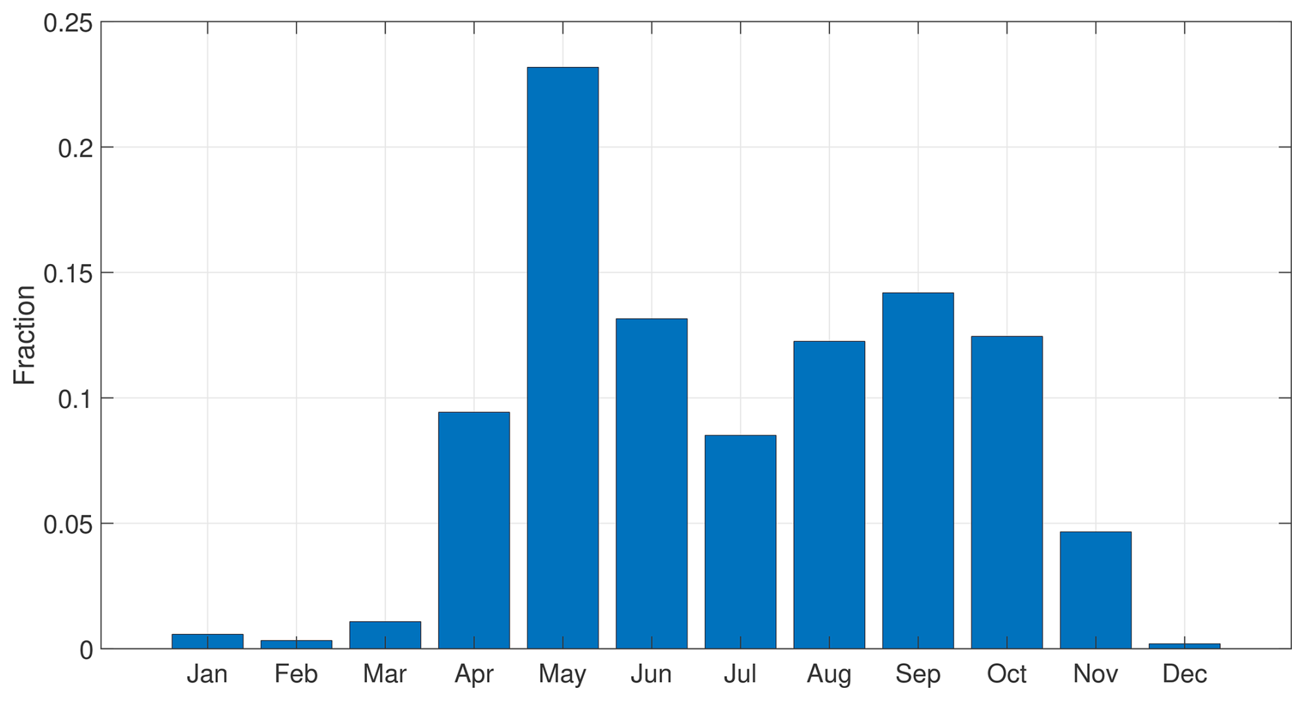
Figure 1 Monthly distribution of open-water gaugings at the 173 hydrometric stations under study.

3 Method

The proposed method follows three steps: (1) adjustment of a single power function in relation to all gaugings available at a given station, (2) segmentation of the original gauging sequence (GS) into sub-sequences to account for possible changes in RC over time, and (3) adjustment of power function according to each GS. The following sections provide further details for each of these steps.

3.1 Adjustment of the rating curve

Gauging measurements at a given station are represented by (h_j,Q_j), with h_j being the measured water levels and Q_j being the corresponding discharges. Parameters of the power function (Eq. 1) used to represent the RCs are estimated by minimizing the mean square relative error (MSRE) defined as (Gupta et al., 2009):

$$\begin{array}{}\text{(2)}& \text{MSRE}={\displaystyle \frac{\mathrm{1}}{N}}\sum _{j=\mathrm{1}}^N{\left[{\displaystyle \frac{Q_{\text{RC}}(h_j;a,b,c)-Q_j}{Q_j}}\right]}^{\mathrm{2}},\end{array}$$

where N is the number of gauging measurements, and $Q_{\text{RC}}(h_j;a,b,c)$ is the estimated discharge from the RC. Relative errors of the estimated discharge were considered. However, this assumption will be further investigated. Parameters of the RC were estimated using the Nelder–Mead non-linear optimization algorithm (Lagarias et al., 1998). RCs are adjusted if six or more gaugings are available.

More than one power function is needed to represent the stage–discharge relationship in some cases (Sect. 3.3 further discusses this point). The RC is therefore represented in these cases by two power functions according to

$$\begin{array}{}\text{(3)}& Q\left(h\right)=\left\{\begin{array}{ll}{Q}_{\mathrm{1}}\left(h\right)=a_{\mathrm{1}}(h-b_{\mathrm{1}}{)}^{c_{\mathrm{1}}}& h\le h^{\prime }\\ Q_{\mathrm{2}}\left(h\right)=a_{\mathrm{2}}(h-b_{\mathrm{2}}{)}^{c_{\mathrm{2}}}& h\ge h^{\prime }\end{array}\right.,\end{array}$$

with $(a_{\mathrm{1}},b_{\mathrm{1}},c_{\mathrm{1}})$ and $(a_{\mathrm{2}},b_{\mathrm{2}},c_{\mathrm{2}})$ being the parameters of the two power functions associated with the water levels below and above h^′, hereafter called the transition level. Continuity at $h=h^{\prime }$ is imposed by setting $Q_{\mathrm{1}}\left(h^{\prime }\right)=Q_{\mathrm{2}}\left(h^{\prime }\right)$. The MSRE (Eq. 2) is therefore minimized by finding the values of $(a_{\mathrm{1}},b_{\mathrm{1}},c_{\mathrm{1}})$, $(a_{\mathrm{2}},b_{\mathrm{2}},c_{\mathrm{2}})$, and h^′ that satisfy the constraint $Q_{\mathrm{1}}\left(h^{\prime }\right)=Q_{\mathrm{2}}\left(h^{\prime }\right)$.

3.2 Temporal partitioning of the gauging series

Changes in RC resulting from modifications of hydraulic or geomorphologic conditions over time were assessed following the procedure presented in Fig. 2. RCs were first estimated using all gaugings at a station. Resulting RCs are hereafter called baseline RCs, as in Darienzo et al. (2021). The analysis is performed when six gaugings or more are available, which is the case for the 173 stations under study. Gaugings are then ranked in chronological order. Consecutive gaugings in chronological order are hereafter called a gauging sequence or GS. The initial GS therefore included all available gaugings at a station. Relative residuals (RRs) between discharges estimated from the adjusted baseline RC and gauged discharges are first estimated (Fig. 2):

$$\begin{array}{}\text{(4)}& {\text{RR}}_j={\displaystyle \frac{Q_{\text{RC}}(h_j;a,b,c)-Q_j}{Q_j}},\end{array}$$

where Q_j and $Q_{\text{RC}}(h_j;a,b,c)$ are the measured and estimated discharges for a given gauging. It is then assumed that changes in hydraulic conditions will manifest through a breakpoint in temporal RR series, and the Pettitt test (Pettitt, 1979) was applied to detect these breakpoints (95 % confidence level). Two additional conditions were considered. Firstly, the test was applied only to gauging sequences with 12 or more gaugings, and, secondly, a breakpoint should not be located within the first or last six gaugings of a GS.

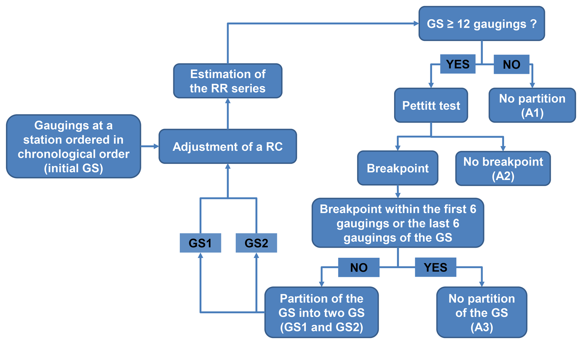
Figure 2 Procedure to assess temporal changes in RC and partitioning of the initial gauging sequences.

The GS is partitioned into two GSs if a breakpoint is detected, and the two previous conditions are satisfied. The first GS encompasses all gaugings before the date of occurrence of the breakpoint, and the second encompasses one all gaugings after the breakpoint. Since the Pettitt test can only detect one breaking point in a GS, the procedure is applied again to the newly partitioned GSs until no further breakpoint point is detected or until one of the previous conditions is not fulfilled (Fig. 2).

Gauging sequences obtained after applying this procedure were classified into three groups (Fig. 2): A1 – GS with less than 12 gaugings (no breakpoint test applied, A2 – GS with more than 12 gaugings and no breakpoint, and A3 – GS with more than 12 gaugings and a breakpoint detected within the first or last 6 gaugings. Group A3 was defined since it suggests that caution is needed when adjusting RCs according to these GSs and if new gaugings are added. The total number of GSs finally obtained at a station corresponds to the number of periods and RCs necessary to represent the stage–discharge relationship over the gauging period at this station.

This procedure was applied to the 173 stations under study. As a result, 96 out of the 173 stations (55.5 %) have one RC (no change in RC over time), 31 stations (18.0 %) had two RCs, while the remaining 46 stations had between three to eight RCs. The total number of RCs is therefore 348 for an average of 2.0 RCs per station and a root mean square relative error (RMSRE) value of 7.3 %, with a 90 % confidence interval ranging from 2.3 % to 18.7 % based on the relative residuals from all stations. The three GSs with more than 12 gaugings and a breakpoint detected within the first or last 6 gaugings (group A3) are not considered in the following.

It should be noted that the proposed procedure cannot account for changes in specific parts of the RC, for instance, those affecting only the low-flow part of the stage–discharge relationship. It also cannot account for a shift in RCs due to progressive riverbed changes, sedimentation, or erosion. Morlot et al. (2014) proposed a method to dynamically upgrade RCs and the associated uncertainties. Jalbert et al. (2011) also proposed an approach based on variographic analysis to estimate the temporal evolution of RCs and the associated uncertainties.

A similar approach was proposed by Darienzo et al. (2021). These authors use a more complex approach based on multi-change point Bayesian estimation and applied the proposed approach to a station on the Ardèche River (France). Although, in principle, it is very similar to the approach previously described, the complexity of the Darienzo et al. (2021) approach limits its large-scale application.

3.3 Adjustment of power functions in relation to gauging sequences

Once the GSs representing the stage–discharge relationship over a specific period have been identified, one must decide if one or two power functions (PFs) are needed to adequately represent the stage–discharge relationship over the entire range of gauged water levels.

Figure 3 presents the general approach used in this study to determine the number of PFs needed to represent the RC (only one or two PFs are considered). It is based on the hypothesis that residuals should be randomly distributed around the RC if it adequately represents the stage–discharge relationship over the whole range of gauged water levels; otherwise, two PFs are needed. Randomness of residuals was assessed by applying a run test, also called a randomness test, to the RR (Eq. 2), sorted in increasing order of gauged water levels. The Wald–Wolfowitz run test (Wald and Wolfowitz, 1940) was used (95 % confidence level). Randomness is tested only if the GS has 12 gaugings or more; otherwise, it is assumed to be random, and one PF is used to represent the RC. If RR series are not random according to the test, the transition level h^′ and the parameters of the two PFs are estimated using Eq. (3). If the estimated transition level is within the six smallest or the six largest gauged water levels then the corresponding GS is put aside for further analysis. Otherwise, the representation by two PFs is kept, and the run test is finally applied to the resulting RR series. No further PF is considered even if the run test concludes that the RR of a two-PF RC is not random (Fig. 3).

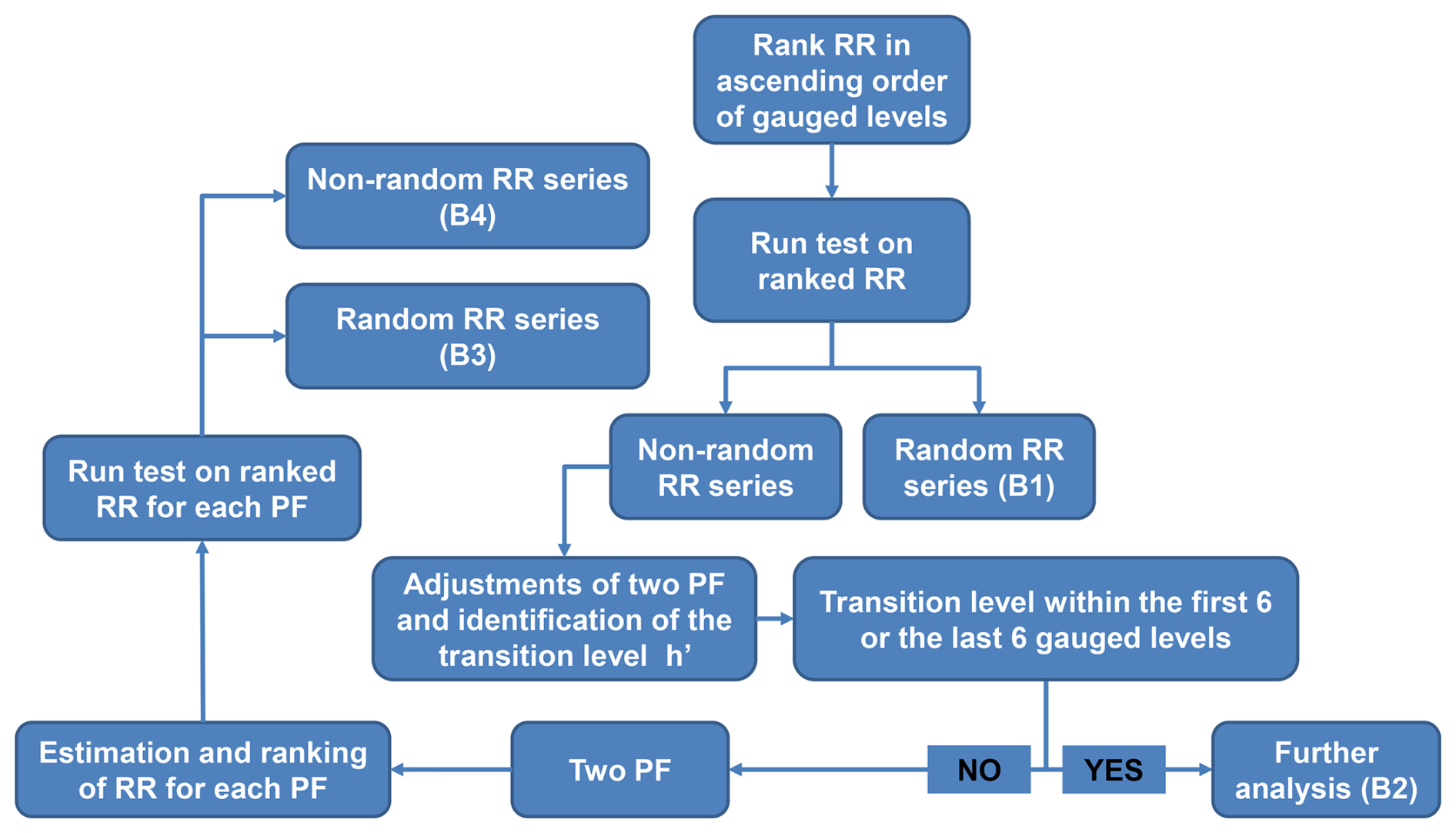
Figure 3 Procedure to assess if one or two power functions (PFs) are needed to represent the stage–discharge relationship of a given GS. The procedure is applied to all GSs with 12 gaugings or more.

After application of the procedure presented in Fig. 3, RCs are classified into the following groups: B1 – RCs represented by one PF (random RR), B2 – RCs represented by one PF with a transition level within the six smallest or the six largest water levels, B3 – RCs represented by two PFs (random RR), and B4 – GSs possibly represented by more than two PFs (non-random RR). RCs of group B4 should eventually be further investigated.

The RCs of the 55 GSs with less than 12 gaugings are represented by one PF (no application of the run test). After applying the procedure presented in Fig. 4, the remaining 290 GSs are classified as follows: 245 in group B1 (one PF), 9 in group B2, 32 in group B3 (two PFs), and 4 in group B4 (more than two PFs). The four RCs of group B4 and the nine of group B2 were excluded from the following analysis.

4 Estimated rating curves

A total of 332 RCs were estimated, with 300 (90.4 %) being represented by one PF and 32 (9.6 %) being represented by two PFs. Distributions of the estimated values of the exponent c of the fitted PFs (Eqs. 1 and 3) are shown in Fig. 4. As previously mentioned, these values can be related to the type of hydraulic control (Le Coz et al., 2014). The mean exponent of RCs represented by one PF is close to 2, a value in between those associated with rectangular and triangular control sections. Also, distributions of c₁ (low-level PF) and c₂ (high-level PF) for RCs represented by two PFs are very different. Larger c₁ values may be related to triangular-like sections, while smaller c₂ values may be related to rectangular-like sections. Values well above $c=\mathrm{8}/\mathrm{3}$ are also reported, especially for the c₁ exponent. Le Coz et al. (2014) mentioned that such values should be considered to be “suspicious”. Hrafnkelsson et al. (2022) also proposed that the exponent value should be within the range [1.0, 2.67]. In our case, 18.0 % of the RCs represented by one PF have exponents larger than $\mathrm{8}/\mathrm{3}$, and this is the case for 53.1 % of those represented by two PFs.

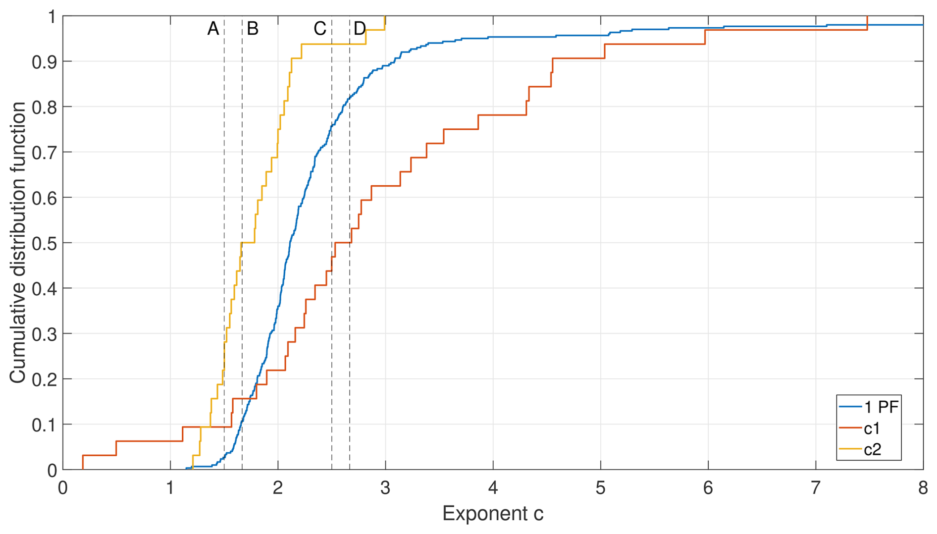
Figure 4 Cumulative distributions of exponent c (Eq. 1) for the 300 RCs represented by one PF and the 32 RCs represented by two PFs (Eq. 3), where c₁ corresponds to lower water levels and c₂ corresponds to higher water levels. Vertical dashed lines correspond to the exponent of the stage–discharge relationships for (A) rectangular weirs ($c=\mathrm{3}/\mathrm{2}$), (B) shallow permanently uniform flow in a rectangular canal ($c=\mathrm{5}/\mathrm{3}$), (C) triangular weirs ($c=\mathrm{5}/\mathrm{2}$), and (D) shallow permanently uniform flow in a triangular canal ($c=\mathrm{8}/\mathrm{3}$). The x axis has been truncated at c=8 for clarity.

The RCs with c>3 or c<1 were further investigated to better understand the conditions leading to these peculiar values. They occur under the following situations:

1. A small number of stage–discharge pairs and a small range of gauged stages. Many unusual c values are observed when the number of gaugings is small, resulting in under-sampled RCs. This is incidentally the case for the three RCs with c<1. Also, in some cases, even if the number of gaugings may seem reasonable, the range of gauged flow and stages remains small. The available stage–discharge pairs “under-sampled” the stage range, and this results in unrealistic c values.

2. Hydrometric stations downstream of dams. Streams downstream of dams often have much smaller flow variability and, therefore, a much narrower range of gauged stages. The largest c values reported in this study correspond to such a situation.

3. Control section upstream of a natural spillway. In some cases, hydraulic control corresponds to a natural spillway. This type of configuration is often observed but could be problematic if the crest of the natural spillway is close to the water surface at a low stage. In such a case, the adjusted b value of Eq. (2) is unrealistic, and a is very small and must be compensated for by a large c value.

4. Compensating effect between a and c parameters of Eq. (2). In some cases, under specific conditions, e.g., when small stages are over-represented compared to high stages, adjusting the CT led to very small a values and large c values. This effect is often observed downstream of dams.

5 Rating-curve uncertainty models

Uncertainties in estimated RCs were first investigated by looking at the RR distribution as a function of normalized discharge, defined as the discharges divided by the mean discharge of each RC, when the 300 one-PF RCs are considered (Fig. 5). Coxon et al. (2015) performed a similar analysis on 26 stable gauging stations in England and concluded that the RRs were adequately represented by a logistic distribution with a discharge-dependent standard deviation. Figure 5 shows that similar results were obtained for the 300 one-PF RCs. Larger uncertainties for high and, especially, low flows are observed, as well as a slight bias for the highest discharges, meaning that discharges estimated from the RC are more likely to have over-estimated gauged values.

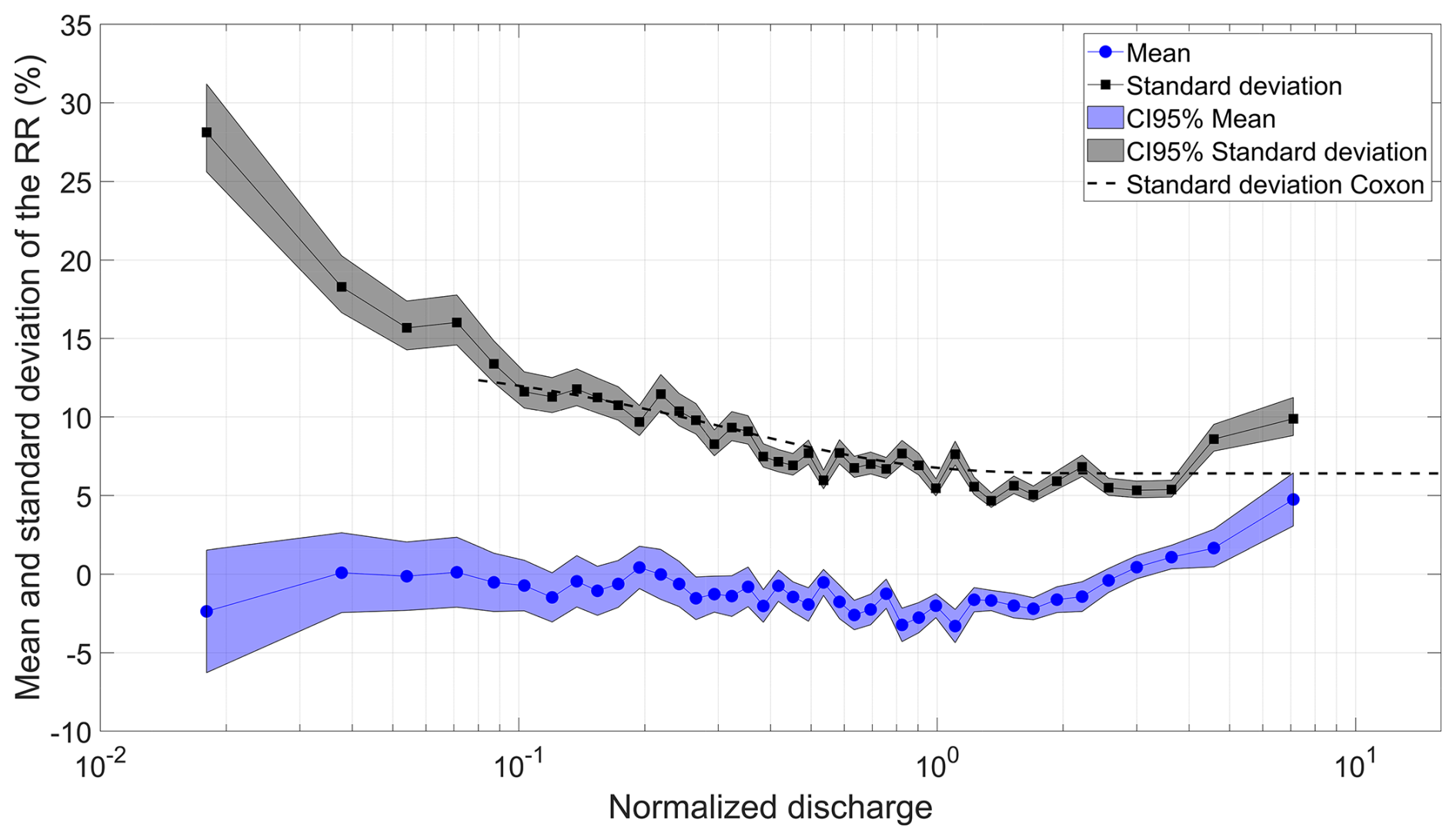
Figure 5 Mean (blue) and standard deviation (black) of the RRs of the 300 one-PF RCs as a function of the mean normalized discharge (each discharge interval includes ≈200 values) with their corresponding 95 % confidence intervals. The dashed curve corresponds to the equation for the standard deviation of the logistic distribution obtained by Coxon et al. (2015). The range of normalized discharges covered by the dashed curve corresponds to the one of Fig. 4 in Coxon et al. (2015). Note the logarithmic x axis.

An L-moment diagram (Hosking and Wallis, 1997) of RR distribution indicates that distribution skewness is close to zero (symmetrical), while kurtosis is much larger than the kurtosis of the normal distribution and even slightly larger than the kurtosis of the logistic distribution (not shown for conciseness), therefore suggesting that the logistic distribution more adequately represents the RR empirical distribution, as in Coxon et al. (2015) (see Fig. 5). Finally, the standard deviations of the RRs for normalized discharge between ≈0.25 and ≈5 are smaller than 10 %, with a minimum value of 5 %, values comparable to reported uncertainties in flow measurements (McMillan et al., 2012).

Uncertainty models for the rating curves were therefore developed based on the previous analysis. Relative normalized stage h^′ is first defined:

$$\begin{array}{}\text{(5)}& h^{\prime }={\displaystyle \frac{(h-h_{\text{min}})}{(h_{\text{max}}-h_{\text{min}})}},\end{array}$$

where h_min and h_max correspond, respectively, to the smallest gauged stage (SGS) and to the largest gauged stage (LGS) at a station; we therefore have $\mathrm{0}<h^{\prime }<\mathrm{1}$.

Normal and logistic distributions were considered for uncertainties in estimated discharges from RCs. Location parameters are set to zero, and four models are considered for the scale parameter σ(h^′) based on the results of Fig. 5:

$$\begin{array}{}\text{(6a)}& {\displaystyle }& {\displaystyle }{\mathit{\sigma }}_{\text{M0}}\left(h^{\prime }\right)={\mathit{\sigma }}_{\mathrm{0}},\text{(6b)}& {\displaystyle }& {\displaystyle }{\mathit{\sigma }}_{\text{M1d}}\left(h^{\prime }\right)={\mathit{\sigma }}_{\mathrm{1}}\exp (-{\mathit{\alpha }}_{\mathrm{1}}{h}^{\prime })+{\mathit{\sigma }}_{\mathrm{0}},\text{(6c)}& {\displaystyle }& {\displaystyle }{\mathit{\sigma }}_{\text{M1i}}\left(h^{\prime }\right)={\mathit{\sigma }}_{\mathrm{2}}\exp \left({\mathit{\alpha }}_{\mathrm{2}}{h}^{\prime }\right)+{\mathit{\sigma }}_{\mathrm{0}},\text{(6d)}& {\displaystyle }& {\displaystyle }{\mathit{\sigma }}_{\text{M2}}\left(h^{\prime }\right)={\mathit{\sigma }}_{\mathrm{1}}\exp (-{\mathit{\alpha }}_{\mathrm{1}}{h}^{\prime })+{\mathit{\sigma }}_{\mathrm{2}}\exp \left({\mathit{\alpha }}_{\mathrm{2}}{h}^{\prime }\right)+{\mathit{\sigma }}_{\mathrm{0}},\end{array}$$

with the parameters σ_m, $m=\mathit{\{}\mathrm{0},\mathrm{1},\mathrm{2}\mathit{\}}$ and α_k, $k=\mathit{\{}\mathrm{1},\mathrm{2}\mathit{\}}$. Model M0 corresponds to a homoscedastic uncertainty model, while models M1d, M1i, and M2 correspond to heteroscedastic models. All parameters are positive, and the condition σ₀>2 % was set to avoid unrealistic standard deviations. Figure 6 presents the relative uncertainties as a function of stage according to these models.

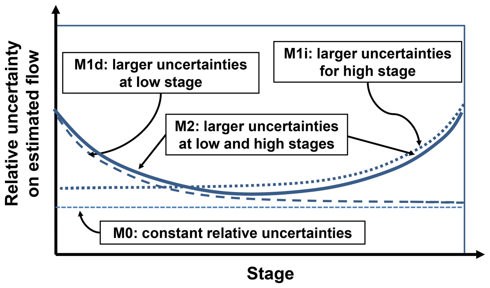
Figure 6 Relative uncertainties in estimated flows as a function of stage for the various uncertainty models: M0 – constant (homoscedastic model; Eq. 6a), M1d – decreasing (Eq. 6b), M1i – increasing (Eq. 6c), and M2 – decreasing for small stages and increasing for large stages (Eq. 6d).

The various uncertainty models have been constructed by combining the normal (N) and logistic (L) distributions with the four models describing the stage dependency of the scale parameters (M0, M1d, M1i, M2). A total of eight models were therefore considered: (1) N-M0, (2) N-M1d, (3) N-M1i, (4) N-M2, (5) L-M0, (6) L-M1d, (7) L-M1i, and (8) L-M2. Therefore, the N-M0 model corresponds to the case where uncertainties in estimated flow are represented by a normal distribution with constant scale parameters (relative uncertainties independent of stage), while L-M1d corresponds to the case where uncertainties in estimated flow are represented by a logistic distribution with decreasing scale parameters as stage increases (larger relative uncertainties at low stages). The parameters of each uncertainty model were estimated by maximizing the corresponding likelihood functions. Results from the different models were then compared using the Bayesian information criterion (BIC; Burnham and Anderson, 2010). The model minimizing the BIC was selected.

Table 1 presents a summary of the results for the 296 RCs with 10 gaugings or more. The normal distribution is the most frequently selected distribution (67.2 %). The homoscedastic model is selected for 75.0 % of the RCs. Models L-M1i, N-M2, and L-M2 are never selected. Consequently, the dominant uncertainty models are the homoscedastic models, namely N-M0 (47.6 %) followed by L-M0 (27.4 %), while the heteroscedastic models, N-M1d and L-M1d, both assuming decreasing relative uncertainties as stage increases, are selected for 24.7 % of the RCs (Fig. 6). These results suggest that the adequacy of the RC in representing the small discharges can be problematic in many cases. The model with increasing uncertainties with stage, N-Mi, is selected once (this case is not considered in the following).

Table 1 Number of RCs (percentages) and mean number of gaugings per RC for each selected uncertainty model. Note that the L-M1i, N-M2, and L-M2 models are never selected. Only RCs with 10 or more gaugings are considered.

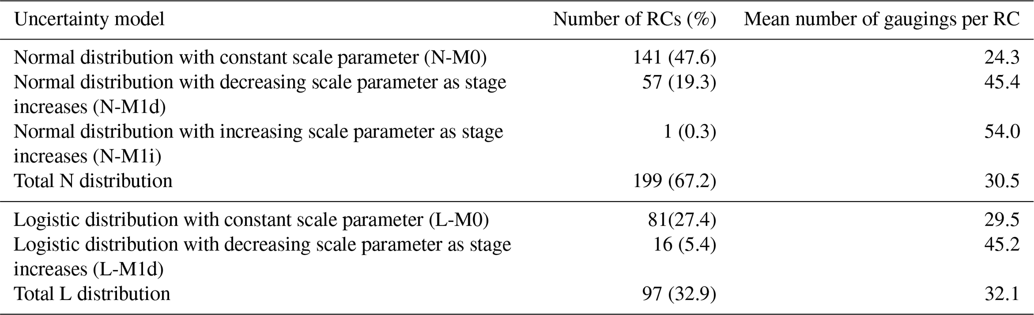
A look at the distributions of the number of gaugings per RC (not shown for conciseness) and at the mean number of gaugings per RC (Table 1) shows that homoscedastic models (M0) are selected more often when the mean number of gaugings is smaller, while heteroscedastic models (M1d and M1i) are selected more often when the mean number of gaugings is larger. This is consistent with the hypothesis that RC based on a larger number of gaugings will more likely explore broader hydraulic conditions and, therefore, more adequately represent the discharge–stage relationship for both low- and high-flow regimes where uncertainties may increase due to a change in control. Figure 7 presents two examples of RCs where the L-M0 and N-M1d models were selected.

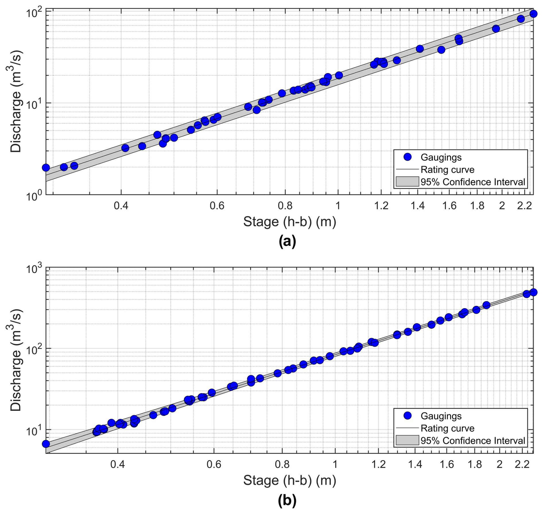
Figure 7 RCs with 2.5 %–97.5 % confidence intervals at (a) Mitchinamecus – 040619 (45 gaugings from 1977 to 2019; L-M0 model with standard deviation of 4.0 %); (b) Matapédia – 011509 (60 gaugings from 1996 to 2022; N-M1d model). Note the y-axis and x-axis logarithmic scales. Stage is expressed as the difference between the level and the reference level (b in Eq. 1).

Figure 8 presents the distributions of standard deviations for RCs with the M0 and M1 uncertainty models. The mean standard deviation for N-M0 models is 6.2 %, with a maximum value of 25.5 %, while the mean standard deviation for L-M0 models is 7.0 %, with a maximum value of 24.5 %. Therefore, 86.4 % of the RCs with homoscedastic uncertainty models have uncertainties smaller than 10 %. For the RCs with M1 heteroscedastic uncertainty models (N-M1d, N-M1i, and L-M1d), uncertainties are smaller than 10 % for a large majority of water levels within the interval $\mathrm{0.1}<h^{\prime }<\mathrm{0.8}$. Uncertainties increase significantly for high and, especially, low stages and can be larger than 20 % in some cases. This shows that caution is needed when estimating flow corresponding to the low and high range of the gauged levels as uncertainties may increase.

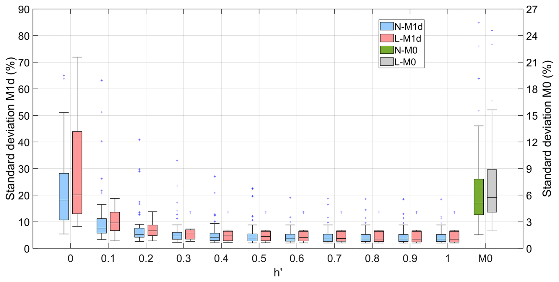
Figure 8 Boxplots of the standard deviations for the 57 and 16 RCs with, respectively, the N-M1d (blue) and L-M1d (pink) uncertainty models as a function of normalized level h^′ (Eq. 5). Boxplots for the 141 and 81 RCs with, respectively, N-M0 (green) and L-M0 (grey) models are displayed on the right-hand side of the graph; refer to the right y axis. The upper limit of the left y axis was set to 90 % for convenience.

6 Summary and conclusions

Stage–discharge relationships at specific control sections or reaches are represented by rating curves (RCs). Hydrometric stations adequately located at these sites record water levels that can be used to estimate discharge using these RCs. These data are crucial inputs for many practitioners responsible for various water management projects such as flood mapping or water supply. Providing uncertainties in estimated discharges from RCs is therefore essential.

Establishing an RC at strategic sites requires that measured discharge and corresponding water levels be monitored over a long period to cover diverse flow regimes. Mathematical functions are then adjusted according to these gaugings and are used to “interpolate” or “extrapolate” the stage–discharge relationship in relation to ungauged water levels. Power functions (PFs) are usually used, but other mathematical functions, such as splines, can be used as well. PFs often appear in formulas describing stage–discharge relationships of standard hydraulic structures such as weirs. The exponent of these PFs, called the hydraulic exponent, can therefore be related to the type of hydraulic controls used.

Many factors must be accounted for when developing an RC, among which are possible irreversible abrupt or long-term changes in stage–discharge relationships due to modifications in watercourse geomorphology, hydraulic controls, or sedimentation. As a result, an RC developed based on past gaugings may be inadequate in representing forthcoming stage–discharge relationships. New gaugings must be realized to update the RC. Another important factor is the adequacy of a single PF in representing the stage–discharge relationship over the whole range of gauged water levels. In some instances, two PFs or more may be necessary to account for possible changes in hydraulic controls.

Many approaches have been proposed in the literature to deal with these issues, but their relative complexity prevents a large-scale application. This paper proposes a simple approach to develop RCs and to estimate corresponding uncertainties that can be readily applied to hydrometric networks. It accounts for possible temporal changes in RC over time and determines if one or two PFs are required to represent the gauged stage–discharge relationship. Uncertainty models for estimated flows from RCs are selected through the analysis of relative residuals of adjusted RCs.

The approach was applied to the Quebec hydrometric network, which includes 173 hydrometric stations mainly located in southern Quebec. The number of gaugings at these stations ranges from 9 to 197 (mean value of 58.3) and covers periods from 3 to 98 years (37.7 years on average). Temporal partitioning of initial gauging sequences was first performed to identify sequences of consecutive gaugings representative of the RCs over specific periods. Single RCs can be used to represent the available gauging period at 96 (55 %) stations of the Quebec hydrometric network, while stage–discharge relationships at 31 (18 %) stations must be divided into two periods and, therefore, be represented by two RCs. The remaining gauging periods at the 46 stations are subdivided into three to eight periods with the corresponding number of RCs. Three RCs were set aside following this analysis. The total number of RCs is therefore 348 for an average of 2.0 RCs per station and 29.0 gaugings per RC.

Adjustment of PFs to these 348 RCs was then carried out. A total of 16 RCs were discarded (more than two PFs or transition levels in the six lowest or six highest gauged levels). Of the remaining 332 RCs, 300 (90.4 %) are represented by one PF, and 32 (9.6 %) are represented by two PFs. The hydraulic exponents for RCs represented by a single PF range from 1.1 to 18.8, with a mean value of 2.5. Most of these values are within the range of standard hydraulic controls (e.g., rectangular or triangular weirs, uniform flow). Hydraulic exponents for RCs represented by two PFs are different, with larger exponents for the low-stage part of the RC and smaller exponents for the high-stage part of RC. These values are most likely to be associated with triangular-shaped sections at low stage (larger exponents) and with rectangular-shaped sections at high stage. Values well above $c=\mathrm{8}/\mathrm{3}$ (associated with triangular-shaped weirs) are also reported for 18.0 % of the RCs represented by one PF and for 53.1 % of those represented by two PFs. Further investigation into these cases is required to better understand the hydraulic controls at these sites and the reasons why such large values are obtained.

Relative residuals (RRs) between the gauged discharges and those estimated from the RCs have been used to identify the appropriate uncertainty model describing the RR distribution of each RC. The normal (N) and logistic (L) distributions were used, and four models were considered to represent the scale parameter dependency with stage, with the first one being with a constant scale parameter (homoscedastic; M0) and the three others being with stage-dependent scale parameters (heteroscedastic), associated with decreasing (M1d), increasing (M1i), and U-shaped (M2) scale parameters as stage increases. Combining the two distributions with the four scale parameter models results in eight uncertainty models ($\mathit{\{}\mathrm{N},\mathrm{L}\mathit{\}}\times \mathit{\{}\text{M0},\text{M1d},\text{M1i},\text{M2}\mathit{\}}$).

The uncertainty model that best fit the RR distributions was identified for each RC. Homoscedastic models are predominantly selected (47.6 % for the L-M0 model and 27.4 % for the N-M0 model), while the preferred heteroscedastic models are the N-M1d (19.3 %) and the L-M1d (5.4 %), both associated with larger relative uncertainties at low stage. Therefore, the adequacy of the RC in representing small discharges could be problematic for many RCs, a situation that may be explained by possible changes in hydraulic controls under a low-flow regime. Only one RC has increasing relative uncertainties with stage, while the U-shaped uncertainty model is never selected. This may be indicative of the fact that high stages are, in many cases, inadequately covered by gauging campaigns, which is not surprising considering the risks and challenges of gauging in such conditions.

Standard deviations for the RCs represented by the given uncertainty models were estimated. The mean standard deviation for N-M0 models is 6.2 %, with a largest value of 25.5 %, while the mean standard deviation for L-M0 models is 7.0 %, with a largest value of 24.5 %. Therefore, the mean uncertainties in RCs represented by homoscedastic models is 6.5 %. For RCs with heteroscedastic models, uncertainties for mid-range gauged stages are comparable to those of homoscedastic models but increase significantly for low stages and can reach values larger than 20 %.

Caution is recommended when using RCs to estimate flow corresponding to the low or high range of the gauging levels used to construct the RCs as uncertainties may rapidly increase and be inadequately represented by the selected uncertainty models. This is important considering the fact that the highest density in available gaugings is for medium-stage levels and that, for operational reasons, high levels are often under-sampled. This could be even more problematic if flows are estimated from the extrapolated part of the RC, i.e., below the smallest or above the largest gauged stage. Gaugings may not or may incompletely cover flow conditions where hydraulic control may change and may not be well-represented by available gaugings and resulting RCs. This could result in bias in the estimated discharges and estimated uncertainties based on the interpolated part of the RC possibly being misleading. This is an important issue for the statistical analysis of flood frequency since the maximum gauged stages are smaller than the 5-year annual maximum measured water level for 52 % of the stations and smaller than the 2-year annual maximum measured water level for 31 % of the stations (this analysis was not presented for conciseness). The estimated annual maximum flow used in the frequency analysis can therefore be highly biased and uncertain. The “representativity” of the range of available gaugings should be assessed to provide guidelines to practitioners responsible for the hydrometric stations for future gauging campaign and data users.

The following points should be further investigated. The proposed procedure to assess the “stationarity” of RCs assumed that, once it is stated that an RC needs to be updated, all past gaugings are discarded and that forthcoming gaugings are used to construct the “new” RC. An alternative approach would be to identify if parts of the RC are still relevant and should be kept when updating the RC, such as in the method proposed by Morlot et al. (2014).

As stated previously, hydraulic exponents of the power function may be linked to the type of hydraulic control at play. Estimated hydraulic exponents obtained after this large-scale application to the Quebec hydrometric network are, for the most part, within the range of values of usual hydraulic structures (weirs, gauging flumes, etc.). However, large values have been reported at some stations. Many of these values may be related to sampling issues and to specific hydraulic configurations. These sites should be further investigated, and the broader issue of the added value of extensive hydraulic analysis (Di Baldassarre and Montanari, 2009; Lang et al., 2010; Mansanarez et al., 2019b) or the quantitative assessment of the hydraulic controls (such as in the BaRatin method proposed by Le Coz et al., 2014) should also be further investigated.