Assessing the value of high-resolution data and parameter transferability across temporal scales in hydrological modeling: a case study in northern China

The temporal resolution of input data and the computational time step are crucial factors affecting the accuracy of hydrological model forecasts. This study presents a four-source hydrological model tailored to the runoff characteristics of the mountainous areas in northern China. Using this model, along with meteorological and hydrological data from seven catchments of varying sizes in northern China, we investigate the impact of different input data resolutions and computational time steps on simulation accuracy as well as the transferability of parameters across different timescales. The results show that (1) the proposed model performs well across different spatial and temporal scales, with an average Nash–Sutcliffe efficiency (NSE) for daily and hourly flow forecasts of 0.93 and 0.85, respectively. (2) For daily streamflow simulations, there was significant improvement in model performance when the data resolution was increased from 24 to 12 h; however, beyond the 12 h resolution, the improvement became negligible. For hourly streamflow simulations, the enhancement in overall flood process accuracy becomes insignificant when the resolution exceeds 6 h, although higher resolutions continue to improve the precision of peak flow simulations. (3) When the computational time step is fixed (e.g., 1 h), model parameters are transferable across different data resolutions; parameters calibrated with daily data can be used in models driven by sub-daily data. However, parameters are not transferable when the computational time step varies. Therefore, it is recommended to utilize a smaller computational time step when constructing hydrological models even in the absence of high-resolution input data. This strategy ensures that the same simulation accuracy can be achieved while preserving the transferability of model parameters, thus enhancing the robustness of the model.

1 Introduction

Hydrological modeling plays a critical role in water resources management, flood forecasting, and climate impact assessments. Accurate simulation of runoff processes is essential for understanding water balance and predicting hydrological extremes. The effectiveness of a hydrological model is influenced by the scale of input data (resolution), the scale of the model's computation, and the scale of the hydrological processes being modeled (López-Moreno et al., 2013; Merheb et al., 2016).

In the past, hydrological modeling typically relied on daily or coarser-resolution data, limiting its applicability to shorter time steps required in scenarios like flash flood forecasting. Models that utilize coarse or artificially enhanced data may introduce biases when applied to finer temporal scales as they may fail to accurately represent the variability and magnitude of key hydrological variables. However, advancements in measurement technologies, including high-frequency automated rain/streamflow gauges and phased-array rain radars, have enabled access to high-resolution rainfall and runoff datasets. Despite these technological advances, the quantitative benefits of high-resolution data in enhancing hydrological model performance remain unclear. For instance, studies on the impact of rainfall data resolution on hydrological models have produced inconsistent results. Kobold and Brilly (2006) found that calibrating hydrological models with sub-daily data and time steps can significantly improve the accuracy of flood forecasting by comparing this method with using daily data and time steps. Jeong et al. (2011) observed similar improvements. Huang et al. (2019) found that increasing spatial resolution has only a marginal or minimal effect on model performance, while high-temporal-resolution data lead to a significant improvement in model performance. However, other studies (Kannan et al., 2007; Ficchì et al., 2016) have found that higher data resolution does not always lead to better model performance. Ficchì et al. (2016) reported that as the timescale is reduced, the improvement in model performance becomes limited, and performance may even degrade. Our previous research (Tudaji et al., 2025) in southern China showed that high-temporal-resolution data do not always have a positive impact on model performance. Nevertheless, that and other related studies acknowledge that further studies across different climate zones and models are necessary to validate and extend the generality of these findings.

Moreover, there remain other unresolved issues regarding data resolution that warrant further investigation. When a certain resolution is selected for a watershed model based on current data availability (or a specific standard) and the model's parameters are calibrated accordingly, the model is essentially considered to be constructed. Nevertheless, should the resolution of subsequent input data deviate from the one employed in the model's creation, the continued reliability of the model's predictive outcomes becomes questionable. There is a need to explore whether the model's parameters were optimized solely to maximize simulation metrics for that particular resolution and whether these parameters can be transferred effectively across different data resolutions. Furthermore, an in-depth investigation into how model parameters adapt to input data of varying resolutions is instrumental in uncovering the specific impacts of these data on hydrological simulation outcomes as well as elucidating the mechanistic aspects of how changes in resolution influence the hydrological simulation process. Reynolds et al. (2017) found that the model calibrated by the daily data performance almost as good as the model calibrated by data at sub-daily resolutions. However, this conclusion was reached under a fixed computational time step, and the study (including the aforementioned studies on input data resolution) also acknowledges that the generality of their conclusions to other regions and models warrants further investigation.

Similarly, another issue that arises when constructing hydrological models is the choice of the model's computational time step. The time dependence and transferability of parameters has been widely studied (Krajewski et al., 1991; Finnerty et al., 1997; Littlewood and Croke, 2008; Reynolds et al., 2017). Recent studies have provided quantitative insights into the relationship between parameters at different computation time steps. Wang et al. (2009) established the relationship between the parameters and the square root of the time step; Jie et al. (2018) established a transformation function between parameter values at different time steps. However, it remains uncertain whether a finer computational time step consistently leads to improved simulation accuracy when the resolutions of input and output are fixed. Moreover, the extent to which parameters can be transferred across different computational time steps without transformation and the existence of an optimal computational time step that maximizes both parameter transferability and model performance are still questions that warrant further investigation.

In light of this background, this study seeks to enhance our understanding of the value of high-resolution data and transferability of parameters across temporal scales in hydrological modeling in a new climatic region using a new model. This study aims to complement studies on the effects of timescales in different climate regions and also provide explanations of the timescale effect of models from a simulation process perspective based on parameter variations. Seven small to medium catchments in northern China (a semi-humid and semi-arid region) were selected as the study area, with the aim of leveraging its unique climate and runoff characteristics to provide new insights into and data analysis for hydrological modeling research and practice. We designed two experiments focusing on the most common hydrological forecasting timescales – daily and hourly – to investigate the value of the high-resolution data on hydrological modeling using data resolutions ranging from 1 to 24 h. Besides, two further experiments, one with various data resolutions and another with various computation time steps, were conducted to assess the transferability of parameters under different conditions. Specifically, this study seeks to address three key questions:

1. What is the necessary resolution of rainfall and streamflow data to provide reliable hourly and daily streamflow simulations?

2. When the computation time step is fixed and hourly, can parameters be transferred when adopting different temporal resolutions of input data?

3. When the temporal resolution of input data is fixed and daily, can parameters be transferred when adopting different computation time steps?

The rest of this paper is structured as follows: Sect. 2 outlines the materials and methodology, including the introduction of study catchments, the hydrological model used, and the experimental designs. Section 3 presents the results of the experiments. Section 4 explains the role of high-resolution data, discusses the transferability of parameters under different conditions, and provides insights into selecting the data resolution and computation time step during the modeling. Finally, Sect. 5 offers concluding remarks and limitations of this study.

2 Materials and methodology

2.1 Study area and data

The Chaobai River, located in northern China and flowing through Beijing, is one of the five major rivers in the Haihe River system of China. In this study, we utilize a set of 7 various size of catchments in the upper reaches of the Chaobai River as the study area (Fig. 1, Table 1), where data quality is relatively high and human activities (such as reservoirs or dams) have minimal impact. Among them, the Xitaizi Basin, the smallest one, is a hydrological experimental catchment. The other six study catchments are the control regions of important hydrological stations located upstream of reservoirs or lakes on the major tributaries in the upper reaches of the Chaobai River basin. Considering the existence of the Baihepu (BHP) reservoir in the Baihe watershed and to exclude human interference and the accumulation of simulation errors, the catchment area between the Baihepu reservoir, Tanghekou (THK), and Zhangjiafen (ZJF) was treated as an independent catchment. The measured outflow from the Baihepu reservoir and the measured flow at THK are used as known boundary conditions in the hydrological model to simulate the flow at ZJF.

The study area is located in a semi-humid, semi-arid region, characterized by a temperate monsoon climate, with highly seasonal precipitation primarily concentrated in July and August, resulting in significant seasonal and interannual variations in river flow. During periods outside the rainy season, the flow is minimal, and in some cases, the river may even run dry. Therefore, we chose the 2021 flood season, which saw significant flood events and has relatively complete data, as the study period for this study.

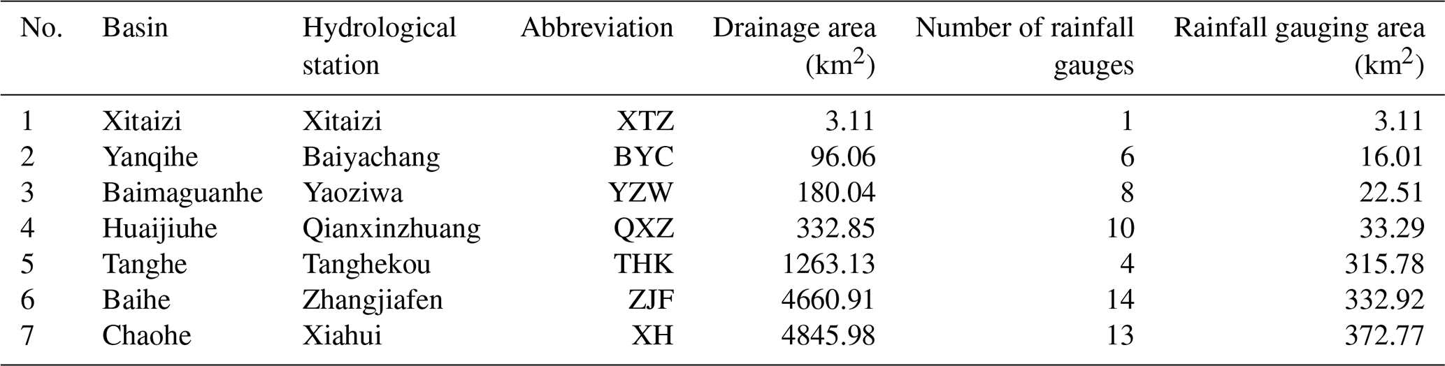
The streamflow and rainfall data were obtained from the Rain and Hydrological Database of Beijing, curated by the Beijing Hydrological Station. When selecting the abovementioned hydrological stations as the outlets for the study basins, the following principles were followed: (1) the station must have discharge data with a resolution finer than hourly during flood events; (2) the upstream control area of the station should be free of water control structures such as reservoirs, dams, or lakes that could significantly affect the natural progression of floods; and (3) the study catchments should cover a range of different scales from a few square kilometers to several thousand square kilometers. The selection of rainfall data followed similar principles, ensuring that each rain gauge station provided complete rainfall data with a resolution finer than hourly throughout the entire storm runoff process. We identified 56 high-quality stations situated within the study catchments from the database. The number of rainfall gauges per catchment varied from 1 to 14, averaging 8 stations. Additionally, the rainfall gauging area – calculated as the catchment area divided by the number of stations – ranged from 3 to 373 km², with an average of 157 km². The Thiessen polygon method (Han and Bray, 2006) was employed to generate the areal rainfall data for each sub-basin in each catchment.

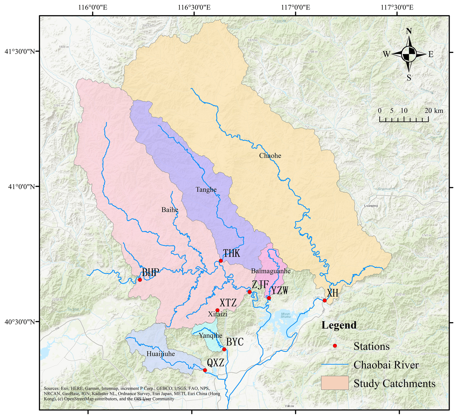
Figure 1 Geographic distribution of study catchments.

Table 1 Information of study catchments and data.

2.2 Hydrological model

The study catchments are located in a rocky mountainous region with severe weathering and high vegetation cover (Zheng et al., 2013; Yu et al., 2017). On the basis of intensive hydrological and isotopic observations from the Xitaizi experimental catchment, Zhao et al. (2019) found that preferential flow in the heavily weathered granite and shallow soils makes up the majority of the stormflow. Recent studies also indicate that subsurface flow is a significant contributor to flood generation (Addisie et al., 2020; Xiao et al., 2020; Wang et al., 2022). To effectively capture the hydrological processes within the study area, a four-source hydrological model was developed, designed to represent multiple hydrological pathways. The model's structural diagram (Fig. 2) illustrates these pathways.

Figure 2 The structural diagram of the hydrological model.

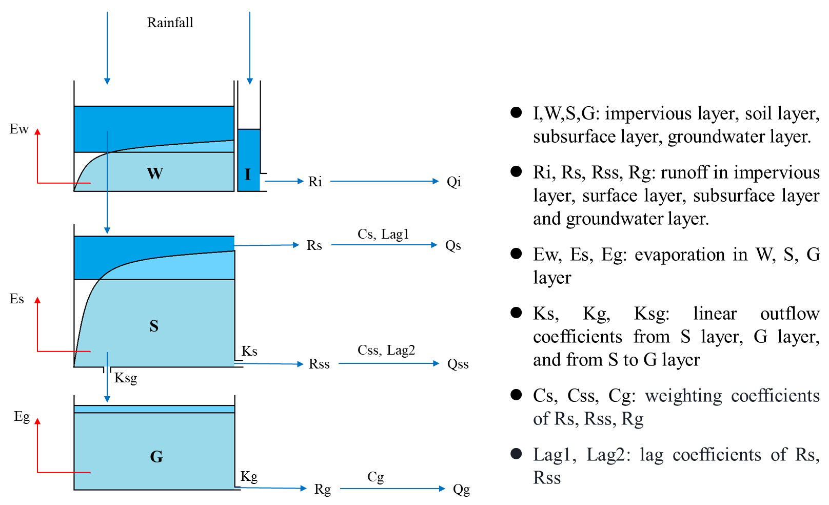
The hydrological model is semi-distributed, which first divides the watershed into multiple sub-basins based on the DEM data. Within each sub-basin, the model further divides the surface layer into two representative units in the horizontal direction: pervious and impervious layers. The impervious layer (I layer) includes waterways, compacted rock layers, and artificial covers (such as concrete roads). Rainfall on the impervious layer is directly converted into runoff impervious layer (R_i) for that time step as follows:

$$\begin{array}{}\text{(1)}& R_{\mathrm{i}}=P,\end{array}$$

where P is the precipitation.

The pervious layer is divided vertically into the capillary water layer (W layer), subsurface layer (S layer), and groundwater layer (G layer). To reflect the spatial variability of water storage capacity in the watershed, the W layer and S layer are enclosed by an exponential curve (Zhao, 1992). Rainfall on the pervious layer is partially routed into the W layer, representing soil moisture, which does not contribute to runoff. Another portion of the rainfall (R) infiltrates into the S layer. Water exceeding the capacity of the S layer is generated as surface runoff (R_s), while the water within the S layer is routed through an outlet, contributing to subsurface runoff (R_ss). The equations for surface runoff and subsurface runoff are as follows:

$$\begin{array}{}\text{(2)}& {\displaystyle }\mathrm{WMM}=\mathrm{WM}\times (\mathrm{1}+B),\text{(3)}& {\displaystyle }A=\mathrm{WMM}\left[\mathrm{1}-{\left(\mathrm{1}-{\displaystyle \frac{W}{\mathrm{WM}}}\right)}^{\frac{\mathrm{1}}{\mathrm{1}+B}}\right],\text{(4)}& {\displaystyle }R=P-E_w+W-\mathrm{WM}\text{if}P-E_w+A\ge \mathrm{WMM},\text{(5)}& {\displaystyle }\begin{array}{rl}R& =P-E_w+W\\ & -\mathrm{WM}\left[\mathrm{1}-{\left(\mathrm{1}-{\displaystyle \frac{P-E_w+A}{\mathrm{WMM}}}\right)}^{\mathrm{1}+B}\right]\\ & \text{if}P-E_w+A<\mathrm{WMM},\end{array}\text{(6)}& {\displaystyle }\mathrm{SMM}=\mathrm{SM}\times (\mathrm{1}+\mathrm{EX}),\text{(7)}& {\displaystyle }\mathrm{AU}=\mathrm{SMM}\left[\mathrm{1}-{\left(\mathrm{1}-{\displaystyle \frac{S}{\mathrm{SM}}}\right)}^{\frac{\mathrm{1}}{\mathrm{1}+\mathrm{EX}}}\right],\text{(8)}& {\displaystyle }{R}_{\mathrm{s}}=R+S-\mathrm{SM}\text{if}R+\mathrm{AU}\ge \mathrm{SMM},\text{(9)}& {\displaystyle }\begin{array}{rl}{R}_{\mathrm{s}}& =R+S-\mathrm{SM}\\ & \times \left[\mathrm{1}-{\left(\mathrm{1}-{\displaystyle \frac{R+AU}{\mathrm{SMM}}}\right)}^{\mathrm{1}+\mathrm{EX}}\right]\text{if}R+\mathrm{AU}<\mathrm{SMM},\end{array}\text{(10)}& {\displaystyle }{R}_{\mathrm{ss}}=S\times K_{\mathrm{ss}},\end{array}$$

where WM, SM, B, and EX are the storage of the W and S layers and their exponential coefficients.

Water in the S layer infiltrates into the G layer. The spatial variability of the groundwater layer's storage capacity is neglected, and groundwater runoff (R_g) is calculated using a linear reservoir approach. The equations for groundwater as follows:

$$\begin{array}{}\text{(11)}& {\displaystyle }{G}_{\mathrm{t}}=G_{t-\mathrm{1}}+S_{\mathrm{t}}\times K_{\mathrm{sg}},\text{(12)}& {\displaystyle }{R}_{\mathrm{g}}=G\times K_{\mathrm{g}}.\end{array}$$

Evaporation occurs in the W, S, and G layers. The evaporation in the W layer is calculated by as follows:

$$\begin{array}{}\text{(13)}& E_w=\mathrm{PET}\times K_{\mathrm{ew}},\end{array}$$

where PET is the mean potential evapotranspiration and K_ew is the linear coefficients. E_s and E_g are calculated by similar equations with the linear coefficients of K_es and K_eg.

Considering the lag time in runoff response to rainfall, the convergence of surface flow and subsurface flow on the hillslopes within a sub-basin is modeled using a lag algorithm. No separate lag time is assigned to groundwater flow as its runoff response to rainfall is slow, and this behavior can be captured through other parameters. No lag time is assigned to the impermeable surface as the travel time of surface water flow within the sub-basin is relatively short and is assumed to not exceed a single time step. Thus, the equations for the flow from all four pathways are as follows:

$$\begin{array}{}\text{(14)}& {\displaystyle }{Q}_{\mathrm{i},\mathrm{t}}=R_{i,t}\times \mathrm{Area}\times \mathrm{imp}/\mathrm{dT},\text{(15)}& {\displaystyle }\begin{array}{rl}{Q}_{\mathrm{s},\mathrm{t}}& =\left[R_{\mathrm{s},\mathrm{t}-\mathrm{1}-\mathrm{lag}\mathrm{1}}\times \mathrm{Cs}+R_{\mathrm{s},\mathrm{t}-\mathrm{lag}\mathrm{1}}\times \left(\mathrm{1}-\mathrm{Cs}\right)\right]\\ & \times \mathrm{Area}\times \left(\mathrm{1}-\mathrm{imp}\right)/\mathrm{dT},\end{array}\text{(16)}& {\displaystyle }\begin{array}{rl}{Q}_{\mathrm{ss},\mathrm{t}}& =\left[R_{\mathrm{ss},\mathrm{t}-\mathrm{1}-\mathrm{lag}\mathrm{2}}\times \mathrm{Css}+R_{\mathrm{ss},\mathrm{t}-\mathrm{lag}\mathrm{2}}\times \left(\mathrm{1}-\mathrm{Css}\right)\right]\\ & \times \mathrm{Area}\times \left(\mathrm{1}-\mathrm{imp}\right)/\mathrm{dT},\end{array}\text{(17)}& {\displaystyle }\begin{array}{rl}{Q}_{\mathrm{g},\mathrm{t}}& =\left[R_{\mathrm{g},\mathrm{t}-\mathrm{1}}\times \mathrm{Cg}+R_{\mathrm{g},\mathrm{t}}\times \left(\mathrm{1}-\mathrm{Cg}\right)\right]\\ & \times \mathrm{Area}\times \left(\mathrm{1}-\mathrm{imp}\right)/\mathrm{dT},\end{array}\end{array}$$

where Q_i, Q_s, Q_ss, and Q_g are the flow from the impervious layer, surface layer, subsurface layer, and groundwater layer, Area is the area of the basin, imp is the proportion of impervious area, and dT is the calculation time step.

The total flow from a sub-basin is the sum of the four flows above. The routing process is modeled using the Muskingum method (Cunge, 1969; Gill, 1978; Yoon and Padmanabhan, 1993), with the equation given as follows:

$$\begin{array}{}\text{(18)}& Q_{\mathrm{i}}^{\mathrm{t}}=C_{\mathrm{1}}{Q}_{i-\mathrm{1}}^{t-\mathrm{1}}+C_{\mathrm{2}}{Q}_{i-\mathrm{1}}^{\mathrm{t}}+C_{\mathrm{3}}{Q}_{\mathrm{i}}^{t-\mathrm{1}}+\left(C_{\mathrm{1}}+C_{\mathrm{2}}\right)Q_{\mathrm{L}},\end{array}$$

where i is the spatial index, t is the temporal index, and Q_L is the lateral flow.

In the Muskingum method, the three parameters C₁, C₂, and C₃ must satisfy the conditions of being within the 0–1 range and their sum equaling 1. To accommodate these constraints within the automatic parameter optimization program, this study reparametrizes the model by optimizing the values of C₁+C₂ and $C_{\mathrm{1}}/(C_{\mathrm{1}}+C_{\mathrm{2}})$, thereby determining the optimal values for the original parameters.

2.3 Experimental design for the value of high-resolution data

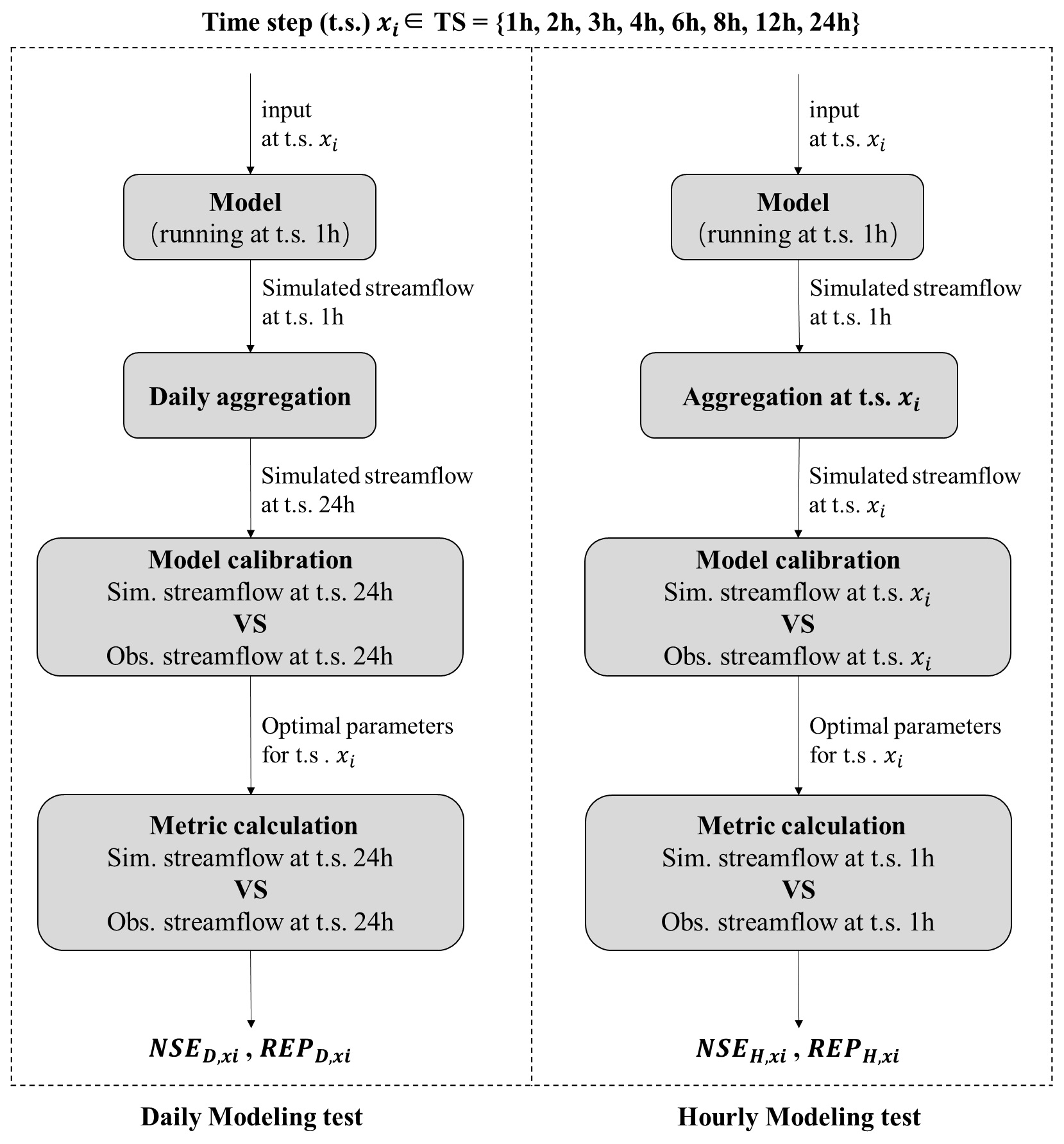
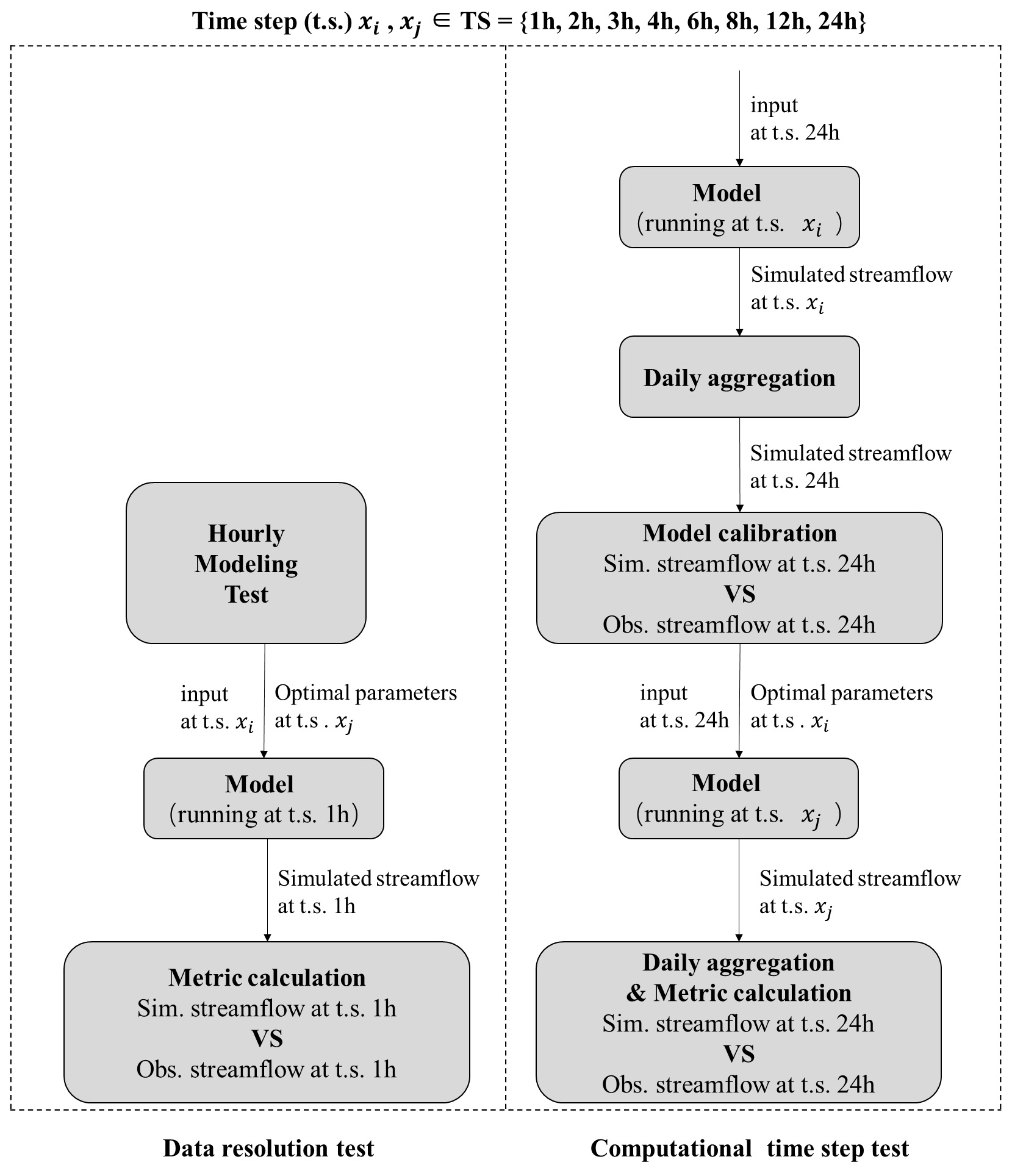
Daily streamflow and hourly streamflow are important modeling targets in hydrological research and practice. To test the value of rainfall and measured streamflow data at different resolutions for simulating streamflow at these two scales, we designed two specific experiments: the daily modeling test and the hourly modeling test. In this context, daily and hourly refer to the target timescales for the model's predictions. The flowchart of the tests is shown in Fig. 3, and the details are as follows:

1. Daily modeling test. This test was designed to investigate the impact of high-resolution rainfall data on daily streamflow simulation. The model was driven by rainfall data at various resolutions (ranging from 1 to 24 h) and calibrated using daily resolution streamflow data. This setup aimed to assess whether (and to what extent) sub-daily rainfall data can enhance daily streamflow simulation.

2. Hourly modeling test. This test was designed to investigate the impact of high-resolution input and streamflow data on hourly streamflow simulation. In this test, the temporal resolutions of input rainfall data and calibration streamflow data were the same and both set to various resolutions (ranging from 1 to 24 h). The model was calibrated using streamflow data with the given temporal resolution, and the hourly streamflow simulated by the calibrated model was then evaluated based on the hourly measured streamflow. This setup aimed to determine the necessary data resolution for providing reliable hourly streamflow simulation.

These experiments aimed to investigate how data resolution affects the accuracy and reliability of streamflow predictions across various temporal scales. To minimize potential impacts from varying computational time steps, the hydrological simulations were consistently set to a 1 h time step for both tests. This standardization was maintained across all cases, with different input data resolutions used. Specifically, all input data, including rainfall, were resampled to a 1 h resolution via prior averaging before driving the model. As a result, the model's original outputs were always produced at an hourly scale.

In the daily modeling test, rainfall data at varying temporal scales were input into the hydrological model to produce simulated hourly streamflow, which was later aggregated to the daily scale for comparison with observed daily streamflow. Model parameters were then optimized by aligning the simulation with observations using the Python Surrogate Optimization Toolbox (pySOT, Eriksson et al., 2019), aiming to maximize the Nash–Sutcliffe efficiency (NSE). The optimization process, iterated via a symmetric Latin hypercube design (SLHD), concluded upon convergence or after reaching a 3000-iteration threshold. After 100 trials, the final parameters were selected based on the maximum NSE. Additionally, after calibration, relative error of peak flow (REP) was computed as a secondary performance metric. These metrics were calculated as follows:

$$\begin{array}{}\text{(19)}& {\displaystyle }\mathrm{NSE}=\mathrm{1}-{\displaystyle \frac{{\sum }_{t=\mathrm{1}}^n\left(Q_{\mathrm{t}}^{\mathrm{obs}}-Q_{\mathrm{t}}^{\mathrm{sim}}\right)}{{\sum }_{t=\mathrm{1}}^n\left(Q_{\mathrm{t}}^{\mathrm{obs}}-\stackrel{\mathrm{‾}}{Q^{\mathrm{obs}}}\right)}},\text{(20)}& {\displaystyle }\mathrm{REP}={\displaystyle \frac{Q_{\mathrm{sim},\mathrm{p}}-Q_{\mathrm{obs},\mathrm{p}}}{Q_{\mathrm{obs},\mathrm{p}}}},\end{array}$$

where $Q_{\mathrm{t}}^{\mathrm{obs}}$ and $Q_{\mathrm{t}}^{\mathrm{sim}}$ are the streamflow for the observed and simulated time series; $\stackrel{\mathrm{‾}}{Q^{\mathrm{obs}}}$ is the average value of the observed streamflow; and Q_sim,p and Q_obs,p are the simulated and observed peak flow, respectively.

The hourly modeling test followed a similar procedure to the daily modeling test, inputting rainfall data at various temporal resolutions into the hydrological model to produce simulated hourly streamflow. This output was aggregated to match the resolution of the input data and compared with the corresponding observed data for calibration. The performance of the calibrated model when simulating hourly streamflow was then assessed by calculating NSE and REP based on the hourly simulated and observed streamflow data.

The flowchart of the experimental tests was illustrated in Fig. 3, where D and H refer to daily and hourly test and x_i is each member of the time step (t.s.) set (TS), which consists of 1, 2, 3, 4, 6, 12, and 24 h. ${\mathrm{NSE}}_{D,x_i}$ and ${\mathrm{REP}}_{D,x_i}$ are the NSE and REP of daily streamflow forced by rainfall at the time step of x_i. Similarly, ${\mathrm{NSE}}_{H,x_i}$ and ${\mathrm{REP}}_{H,x_i}$ denote NSE and REP for hourly streamflow at the time step of x_i.

After tests, the paired two-sample t test, a widely used statistical method to determine whether the means of two related groups of samples are significantly different (e.g., Xu et al., 2017), was adopted to test whether the performance of the hydrological model based on high-resolution data was significantly improved.

Figure 3 Flowchart of the daily modeling and hourly modeling tests.

2.4 Experimental design for parameters transferability

To test the potential impact of the resolution of training data and the computational time step on the calibration of model parameters as well as the transferability of these parameters across different timescales, we designed two tests: the data resolution test and the computational time step test. The flowchart of the tests is shown as Fig. 4, and the details are as follows:

1. Data resolution test. In this test, the model's computational time step was fixed at 1 h, while the temporal resolution of the input and measured streamflow varied from 1 to 24 h (as in the hourly test). Previously, optimal parameter sets, ${\mathrm{Par}}_{x_i}$, were obtained under varying resolutions (x_i) of input and measured streamflow data in hourly modeling tests. In this data resolution test, the optimal parameter set obtained at one resolution (referred to as the pre-transfer resolution) was used to drive the model with input data at another resolution (referred to as the post-transfer resolution), resulting in hourly simulated streamflow. The simulation accuracy, measured by NSE, was then calculated. By comparing the changes in the simulation metrics obtained by a same set of parameters and different input resolutions, the transferability of the parameters across varying resolutions was tested.

2. Computational time step test. In this test, the model's computational time step varied from 1 to 24 h, while the temporal resolution of the input rainfall and measured streamflow data was fixed as 24 h. Firstly, input data at the resolution of 24 h were fed into the model, and the model was run at varied time steps, resulting in simulated streamflow at varied time steps. Next, the simulated streamflow was aggregated daily, and the model parameters were calibrated based on observed daily streamflow. In this way, the model parameters under different computational steps were obtained. Then, the optimal parameter set obtained at one computational time step (referred to as the pre-transfer computational time step) was used to drive the model at another computational time step (referred to as the post-transfer computational time step), and NSE was calculated based on the simulated daily streamflow obtained at this time step. By comparing the changes in simulation metrics, the transferability of parameters obtained at one computational time step to another was tested.

Figure 4 Flowchart of the data resolution and computational time step tests.

3 Results

3.1 The value of high-resolution data

The results of the daily and the hourly modeling tests are shown in Fig. 5. Panels (a) and (b) represent the NSE and absolute values of REP in the daily modeling test, respectively. Panels (c) and (d) depict these two metrics in the hourly modeling test. In the daily test, the average NSE obtained by various data resolutions varied in the range of 0.91–0.94. The model performed the worst when using 24 h resolution data, but even then, the lowest NSE value was 0.82 in the Yanqihe catchment at BYC station, and in the other six catchments, NSE exceeded 0.89. As for REP, the average $\left|{\mathrm{REP}}_{\mathrm{D}}\right|$ at various data resolutions ranged between 2 % and 4 %, indicating high accuracy in the simulation of peak flow at the daily scale. In the hourly modeling test, the metrics got slightly worse compared with the daily test. The average NSE across various data resolutions ranged from 0.78 to 0.87. The model performed the worst when using 24 h resolution data, with the lowest NSE of 0.64, but NSE exceeds 0.8 in five of the study catchments. The model produced an NSE higher than 0.83 in 6 catchments when using 1 h rainfall and streamflow data. The average $\left|{\mathrm{REP}}_H\right|$ varied in the range of 16 %–27 %. Compared to the daily modeling test, the model's accuracy in simulating peak flow declined noticeably in hourly modeling as the evaluation was more strict. Overall, these results demonstrated the high performance and reliability of the model in these catchments, with high NSE and low $\left|\mathrm{REP}\right|$.

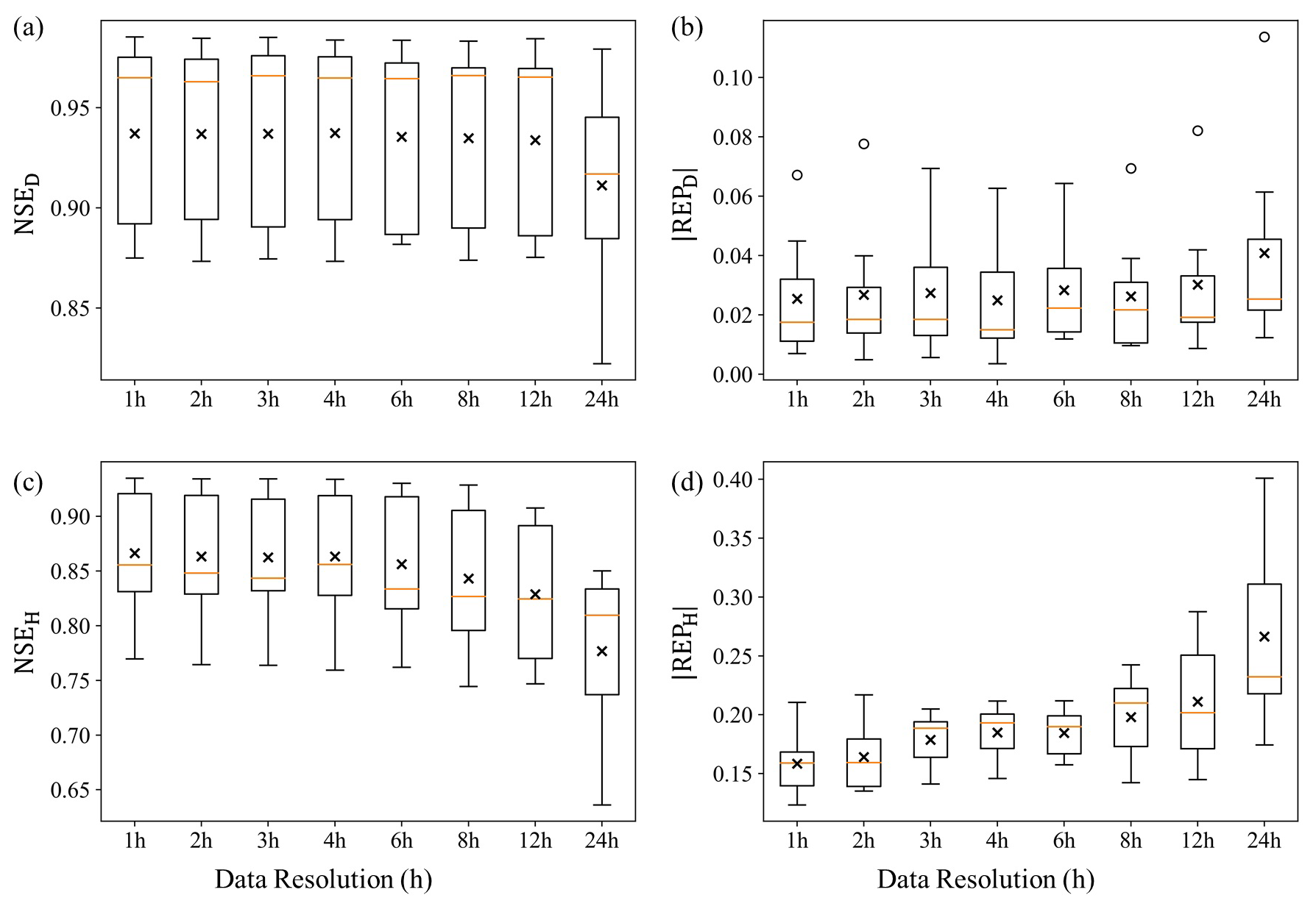
Figure 5 Box plot of NSE and $\left|\mathrm{REP}\right|$ in the daily and the hourly modeling tests across seven catchments.

In both daily and hourly modeling tests, there was an obvious improvement in model performance when the data resolution increased. For instance, in the daily modeling test, when the data resolution shifted from 24 h to sub-daily 12 h, the average NSE increased from 0.91 to 0.93, and the average $\left|\mathrm{REP}\right|$ decreased from 4.08 % to 3.02 %. In the hourly modeling test, the improvement was more obvious. The average NSE increased from 0.78 to 0.83, and the average $\left|\mathrm{REP}\right|$ decreased from 27 % to 21 % when the data resolution shifted from 24 to sub-daily 12 h. But such an improvement got increasingly limited as the resolution increased further.

To quantify the difference in the model performances when adopting data with different resolutions, paired two-sample t tests were conducted, and the results are shown in Table 2. In the daily modeling test, significant improvement (at the 0.05 significance level) on streamflow simulation was brought by sub-daily (1–12 h) resolution rainfall data compared to the daily data as indicated by the low p values in the last row of Table 2a and b. However, compared to 12 h resolution, only 1 h resolution brought a significant improvement in NSE at the significance level of 0.05. As for $\left|\mathrm{REP}\right|$, there were significant differences in $\left|\mathrm{REP}\right|$ at 2 and 8 h resolutions compared to 12 h resolution. Overall, the results suggested that for daily streamflow forecasting, continuously increasing rainfall data resolution beyond the 12 h threshold did not bring significant improvement on model performance. That is, the simulated daily streamflow obtained from a model driven by 12 h rainfall input had comparable reliability to that forced by 1 h data, and the effect of rainfall data with a temporal resolution exceeding 12 h on enhancing daily forecasted flow was negligible.

Similar results were observed in the hourly modeling test (Table 2c and d). Compared to the daily data, utilizing higher-resolution data effectively enhanced the model's forecasting performance for hourly streamflow. Specifically, regarding NSE, there were significant differences in the model's performance when using 8 h resolution data compared to that obtained by 2 to 6 h resolution data. But when the data resolution reached 6 h or higher, there were no statistically significant differences in NSEs, indicating that further increasing the resolution did not consistently enhance overall simulation accuracy. Consequently, taking NSE as the performance metric, simulated hourly streamflow obtained by a model driven and calibrated by 6 h data was comparably accurate to that obtained by higher-resolution data. Data with a resolution higher than 6 h did not provide significant additional value. Compared to NSE, the improvement in $\left|\mathrm{REP}\right|$ was more pronounced with the increase in data resolution in the hourly modeling test. Compared with daily (24 h) resolution data, all sub-daily resolution (1–12 h) data showed significant improvement in $\left|\mathrm{REP}\right|$ (at 0.05 significance level). Comparing the effects of sub-daily scale data, although there was no significant difference in $\left|\mathrm{REP}\right|$ when resolutions were close (e.g., 6 and 8 h resolutions), significant differences in $\left|\mathrm{REP}\right|$ still existed when the resolution was sufficiently high (e.g., 1 h) compared to other resolutions. For instance, the first column of Table 2d indicates that only $\left|\mathrm{REP}\right|$ obtained with 2 h resolution data showed no statistically significant difference when compared to 1 h resolution data. This suggests that continuously increasing the data resolution has a greater value in improving the accuracy of predictions of peak flow.

Table 2 P values of the paired two-sample t tests for each metric. Bold values indicate p < 0.05, with ^* representing $\mathrm{0.01}\le p<\mathrm{0.05}$ and ${}^{**}$ representing p < 0.01.

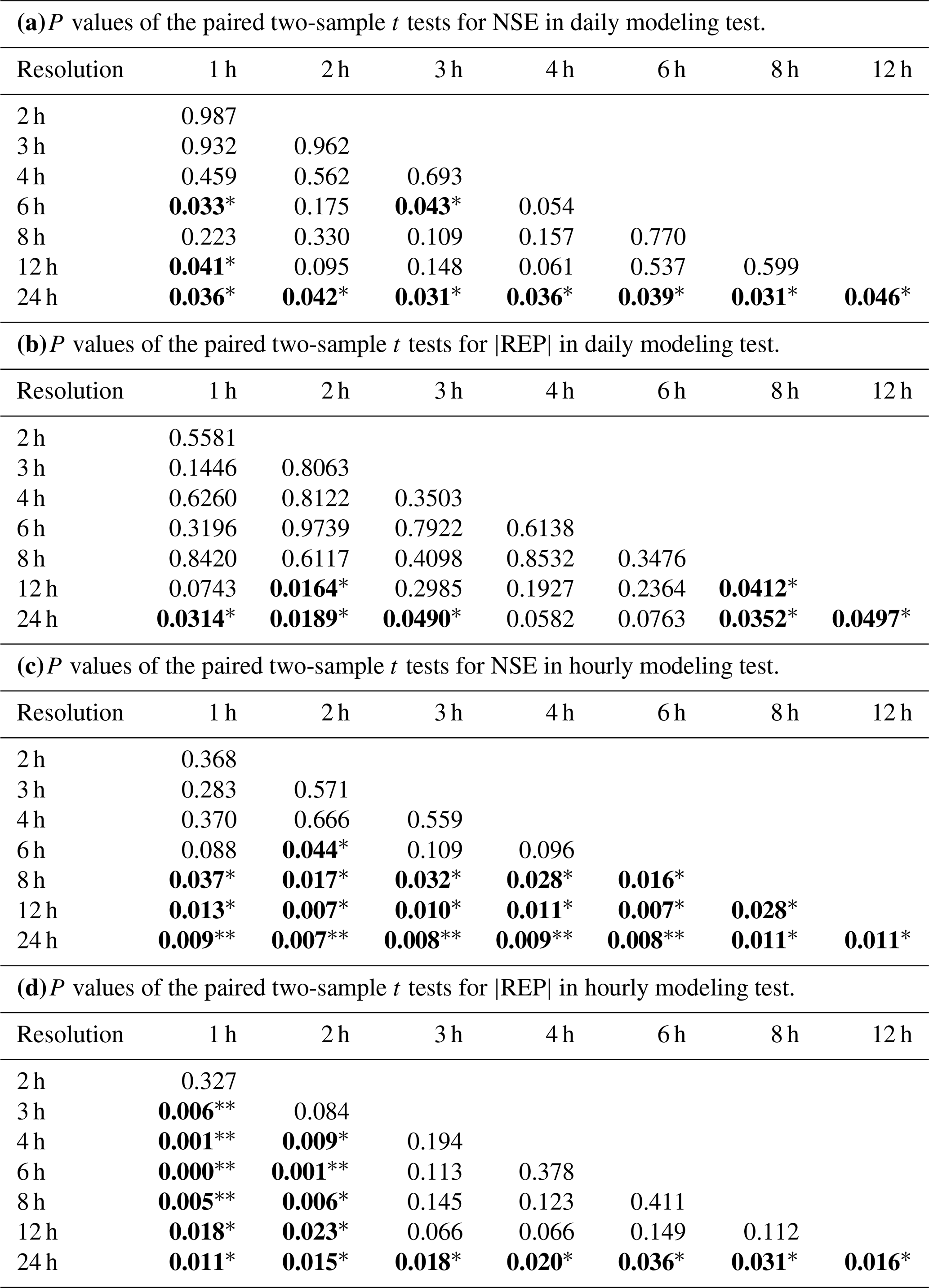
Note: ${}^{**}$ and ^* indicate a significance of 0.01 and 0.05.

3.2 Parameters transferability across data resolutions

The optimized model parameters at various data resolutions were obtained under a fixed computational time step of 1 h in the hourly modeling test. To assess the transferability of these parameters under different data resolutions, the data resolution test was conducted following the experimental design outlined in Sect. 2.4. The results are shown in Fig. 6. In each panel, each curve represents NSE values obtained when the optimal parameters calibrated from a specific input resolution are transferred (without any transformation) to drive the model with other input resolutions.

First, when examining the differences among the curves, it was found that in most catchments, the curve representing the 24 h resolution consistently fell below the others. This aligns with the results from the previous section, indicating that the model's performance was the lowest when using 24 h resolution rainfall and streamflow data. When these parameters are transferred to other resolutions, they also exhibit the lowest performance.

In all catchments except for XTZ, when parameters calibrated with a specific data resolution were transferred to other resolutions, simulation accuracy improved as the resolution of the data used increased. Notably, when the resolution increased from 24 to 12 h, NSE showed the most significant improvement. However, when the input data resolution ranged between 1 and 8 h, NSE remained relatively stable. This observation is consistent with the results and conclusions from Sect. 3.1. Even though there were some variations in model performance when parameters were transferred to other timescales, the performance remained acceptable, with the lowest NSE still exceeding 0.5. This lowest NSE occurred at the QXZ station when the pre-transfer resolution is 6 h and post-transfer resolution is 24 h. When the post-transfer resolution was finer than 24 h, NSE at QXZ was consistently above 0.7. Overall, after parameter transfer, the model continues to demonstrate satisfactory simulation performance.

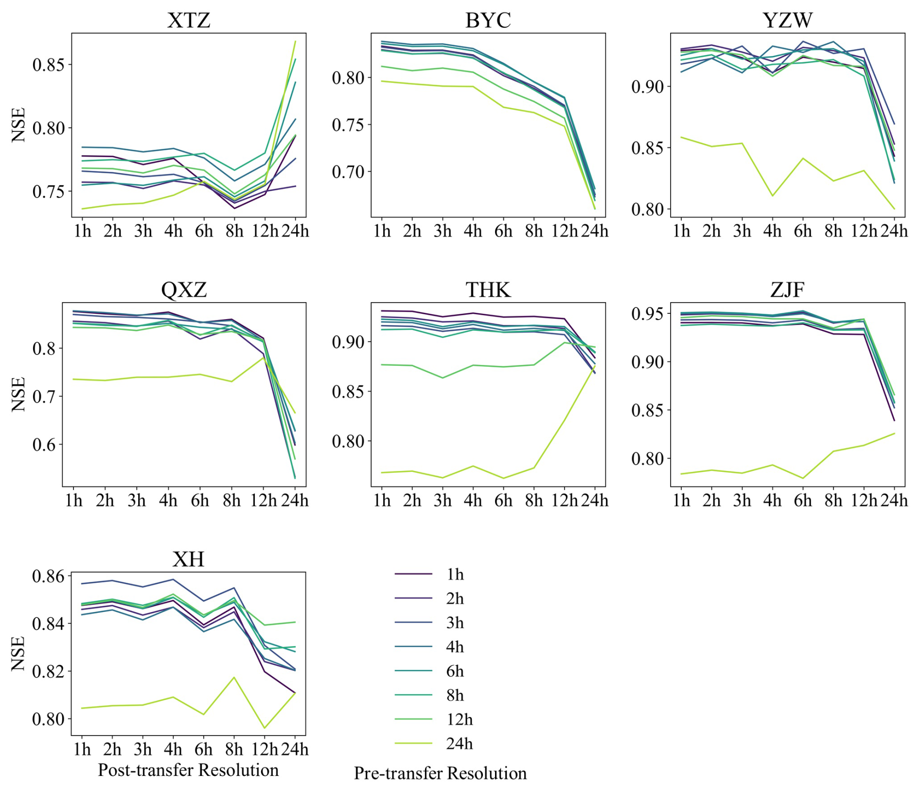
Figure 6 NSE values after transferring the parameters obtained at one resolution to other resolutions.

3.3 Parameters transferability across computational time steps

To assess the transferability of parameters under different computational time steps, the computational time step test was conducted following the experimental design outlined in Sect. 2.4. The results are shown in Fig. 7. The value in the row i and column j represents the NSE value obtained when transferring the parameters calibrated with a computation time step of x_i directly to a model with a computation time step of x_j (x_i, $x_j\in \mathit{\{}\mathrm{1},\mathrm{2},\mathrm{3},\mathrm{4},\mathrm{6},\mathrm{8},\mathrm{12},\mathrm{24}\mathrm{h}\mathit{\}}$, referred to as pre-transfer and post-transfer computational time step, respectively). The values on the diagonal represent NSE values obtained when running the model with a specific computational time step and calibrating the parameters with daily streamflow. In this case, the parameters are not transferred (i.e., the pre-transfer and post-transfer time steps are the same). First, the values on the diagonal are all greater than 0.7, with most exceeding 0.85, and the average is 0.88. This indicates that the model performs well across different computation time steps, further confirming its reliability. Secondly, within each basin, the values on the diagonal are very close to each other, implying that when both the input rainfall data resolution and the output streamflow resolution are at the daily scale, nearly identical simulation accuracy can be achieved regardless of the computation time step used (within the 1–24 h range).

When parameters calibrated at one computation time step were transferred to other computation time steps (values in the same row in Fig. 7), NSE values varied significantly. Compared to the results with the data resolution test in Sect. 3.2, the variation in NSE under the varying computation time step was much greater. In many cases, the NSE value after transferring parameters was even less than 0, indicating that the model parameters lose their transferability (with unreliable accuracy) when the model's computation time step is varied. Notably, in each subfigure, the values in the lower-left part are even lower than those in the upper-right part, suggesting that the model's performance is particularly unreliable when parameters calibrated at larger computation time steps are transferred to smaller ones.

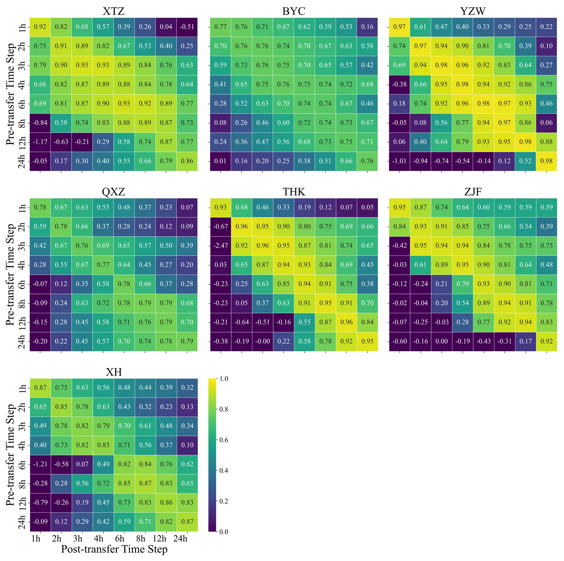
Figure 7 NSE values after transferring the parameters obtained at one computation time step to other time steps.

4 Discussion

4.1 Potential factors for the limited impact of high-resolution data

The results indicate that increasing input data resolution, especially from 24 to 12 h, significantly boosted simulation accuracy for daily streamflow, which is consistent with expectations regarding the benefits of high-resolution data. However, beyond the 12 h mark, performance became marginal or even declined. Similar patterns emerged in hourly simulations, where benefits of finer-than-6 h data were negligible or negative, contradicting the intuitive expectations that higher-resolution data always enhances hydrological models. Similar findings were reported by previous studies that investigated the effects of temporal resolution on hydrological models across different regions and model types. Ficchì et al. (2016) explored 240 catchments in France using the GR4 rainfall–runoff model across eight temporal scales, ranging from 6 min to 1 d. Their analysis revealed that, on average, finer-resolution data provided no additional value when model outputs were aggregated to a 6 h reference scale. Similarly, Reynolds et al. (2017), while calibrating the HBV model in two small central American basins, observed that using daily streamflow data produced results comparable to those obtained at sub-daily resolution.

Another notable result we observed is that in the hourly test, when the resolution reached or exceeded 6 h, there was no significant improvement in NSE, while $\left|\mathrm{REP}\right|$ ceased to improve significantly only the resolution reached 2 h. In our previous study in southern China, both of these threshold resolutions were found to be 6 h. On the one hand, this indicates that the threshold resolution for limiting further improvements in model performance depends on the evaluation metrics used as each metric emphasizes different aspects of the time series and comes with its own limitations and trade-offs (e.g., Schaefli and Gupta, 2007; McMillan et al., 2017; Fenicia et al., 2018). The benefits of high-resolution data may not be fully captured by a single measure, and using different metrics to assess the impact of high-resolution data on model performance may lead to varying conclusions. On the other hand, a deeper investigation into the causes may point to differences in the climate and runoff characteristics of the two study regions. Southern China features subtropical and tropical monsoon climates, with warm, humid conditions and abundant, evenly distributed rainfall (Fan et al., 2019; Domrös and Peng, 2012). Annual precipitation typically exceeds 800 mm (averaging 1500 mm in our previous study area), classifying it as a humid region. Flood generation in this kind of humid region is predominantly governed by saturation excess (Dunne et al., 1975; Zhao, 1992; Manfreda, 2008). In contrast, northern China experiences a temperate monsoon climate with lower and more concentrated rainfall. Annual precipitation is generally below 800 mm (averaging 600 mm in this study area), making it a semi-humid-to-semi-arid region where flood generation is primarily driven by infiltration excess and subsurface preferential flow (Zhao, 1992; Zhao et al., 2019; Fu et al., 2024). Hence, in arid catchments the enhancement of temporal resolution of data is more conducive to improving the model's performance in simulating peak flow as compared to humid catchments, as high-temporal-resolution data enable a more precise capture of variations in precipitation and discharge, particularly at peak values.

While the catchments and models vary across different studies, the overall findings are largely consistent, suggesting that simply increasing the data resolution does not always lead to better model performance. Several factors may limit the additional benefits of higher-resolution data. Firstly, a straightforward reason could be the choice of the evaluation metric. In the hourly modeling test, when the resolution exceeded 6 h, there was no significant improvement in NSE, but $\left|\mathrm{REP}\right|$ showed a marked change. In some cases, different metrics may be in conflict with each other, making it impossible to optimize them simultaneously. The benefits of high-resolution data for a model might not be fully captured by the commonly used metrics and may require alternative indicators for quantification. Using different metrics to assess the impact of high-resolution data on the model could lead to varying conclusions, highlighting the complexity and multifaceted nature of the benefits conferred by enhanced data granularity. Secondly, due to spatial and temporal autocorrelation in variables like rainfall and runoff, increasing resolution beyond a certain threshold may not provide effective new information. There may be no significant difference between actual high-resolution data and high-resolution data obtained by resampling from coarser data. The extent of this difference is related to the characteristics of the climate of the catchment and its runoff generation processes. Thirdly, model input data, particularly rainfall, may have a lower signal-to-noise ratio at higher temporal resolutions due to difficulties in data validation and increased uncertainty in areal average rainfall estimates (Ficchì et al., 2016; Moulin et al., 2009). Besides, since hydrological models inherently simplify natural processes, they may dampen the natural smoothing effect seen in rainfall–runoff interactions. As a result, using high-resolution temporal data to drive the model could introduce excessive variability in the simulated flow, potentially degrading the model's performance. Finally, the model's structure might not be adequately designed to handle the added complexity that comes with shorter time steps. Melsen et al. (2016) pointed out that calibration and validation time intervals should align with the spatial resolution to accurately capture the relevant processes. Some empirical formulas within the model may not be applicable at shorter timescales.

4.2 Parameters transferability across data resolutions

The results in Sect. 3.2 indicate that when the computation time step is fixed at 1 h, the model demonstrates good performance even when parameters are transferred to input conditions with different resolutions. As shown in Fig. 6, in most cases, as the input resolution improves, NSE also increases. However, some exceptions were found. At hydrological stations such as the THK and ZJF, when using parameters calibrated with 24 h data, there was an increase in NSE as the rainfall resolution decreased. At the XTZ station, NSE also increased when the rainfall resolution dropped below 8 h regardless of the parameters used. This anomaly was particularly pronounced at the THK station. Conversely, at the BYC station, NSE consistently decreased as the rainfall resolution decreased across all parameters. We selected the THK and BYC stations as representative cases and compared the streamflow processes driven by 1 h and 24 h rainfall resolutions using parameters calibrated with 24 h data (as shown in Fig. 8). Based on these flow processes, we explored the reasons behind these observed phenomena.

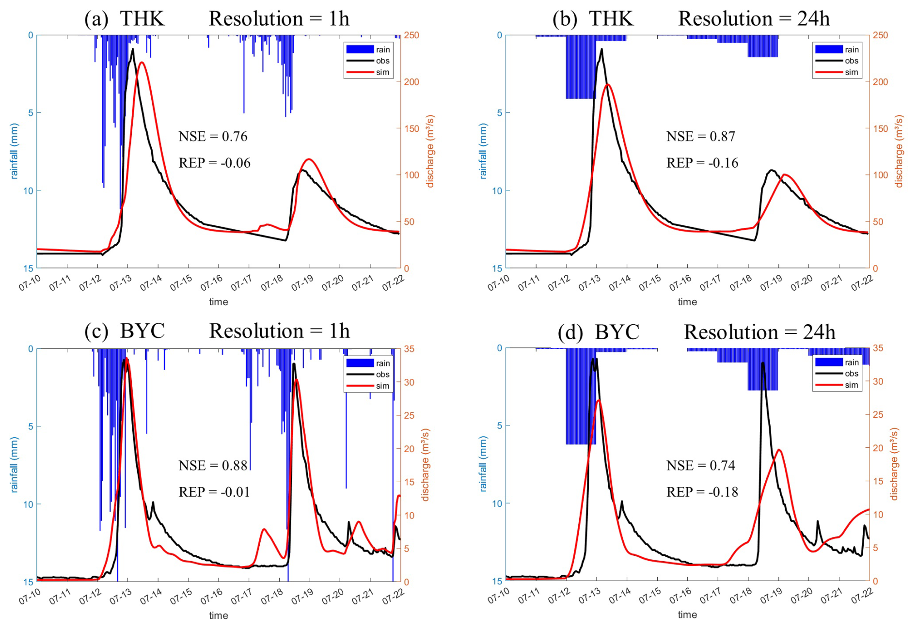
Figure 8 Streamflow processes at THK and BYC driven by 1 h and 24 h rainfall resolutions using parameters calibrated by 24 h data.

In Fig. 8a and b, the model parameters are calibrated using 24 h data, but the rainfall data used to drive the model are at resolutions of 1 and 24 h, respectively. The same setup is applied in Fig. 8c and d. We observed that when using 1 h resolution rainfall data, the simulated value of the first flood peak at the THK station was closer to the measured value even though NSE at 1 h resolution was statistically lower than NSE at 24 h resolution.

To more comprehensively evaluate the simulation accuracy and the impact of different parameters, we conducted further analysis. As mentioned in Sect. 2.2, we ran 100 iterations using the pySOT program for parameter calibration, which resulted in 100 sets of optimized parameters. Using these 100 parameter sets and the rainfall data at both 1 and 24 h resolutions, we evaluated the simulation accuracy of the THK station's streamflow using NSE, KGE (Kling–Gupta efficiency; Gupta et al., 2009), and REP indicators, as shown in Fig. 9.

Among the results obtained using the 100 sets of optimal parameters, NSE values driven by 1 h resolution rainfall data were generally lower than those driven by 24 h resolution rainfall, with average values of 0.63 and 0.77, respectively. The KGE values were relatively close under both resolutions, with average values of 0.81 and 0.84, respectively. As for the $\left|\mathrm{REP}\right|$ indicator, the trend was reversed, with 1 h resolution rainfall data yielding better results than 24 h resolution data, with average $\left|\mathrm{REP}\right|$ values of 9 % and 16 %, respectively. Based on the runoff processes shown in Fig. 8 and the different indicators in Fig. 9, we infer that the observed phenomenon, where simulation accuracy decreases as resolution increases, may be related to the evaluation metrics used and the flood characteristics of the basin.

Compared to the BYC station, the THK station exhibited a slower streamflow process during flood events, particularly during the recession phase. We defined a concept similar to the half-life period, denoted as T_hl, to characterize the rate of flood recession. T_hl is the time taken for the streamflow to decay from its peak to half of the peak value. At the THK station, T_hl is 16 h, while at the BYC station, T_hl is 8 h, indicating that the flood recession at THK is slower than at BYC. In catchments with a more gradual recession, observed streamflow at a 24 h resolution does not provide as much effective information for the model's calibration as higher-resolution data do. Furthermore, when 24 h resolution rainfall is used as input and 1 h as the computational time step, the model tends to produce a smoother simulated streamflow process since it distributes the rainfall evenly over each hour. Consequently, parameters related to flow routing are not accurately calibrated. As a result, when the model is driven by higher-resolution rainfall data such as 1 h, larger errors occur at the predicted peak time. However, when using 24 h resolution rainfall data, the smoothing effect of the 1 h computational time step leads to a simulated recession process that more closely matches the observed values, thus improving NSE.

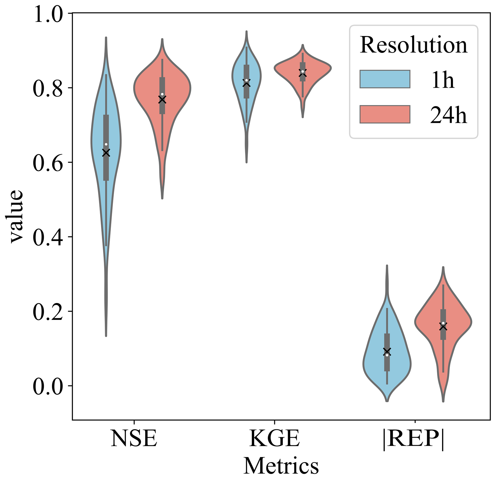
Figure 9 Metrics at the THK station using 100 sets of parameters and different resolutions of rainfall.

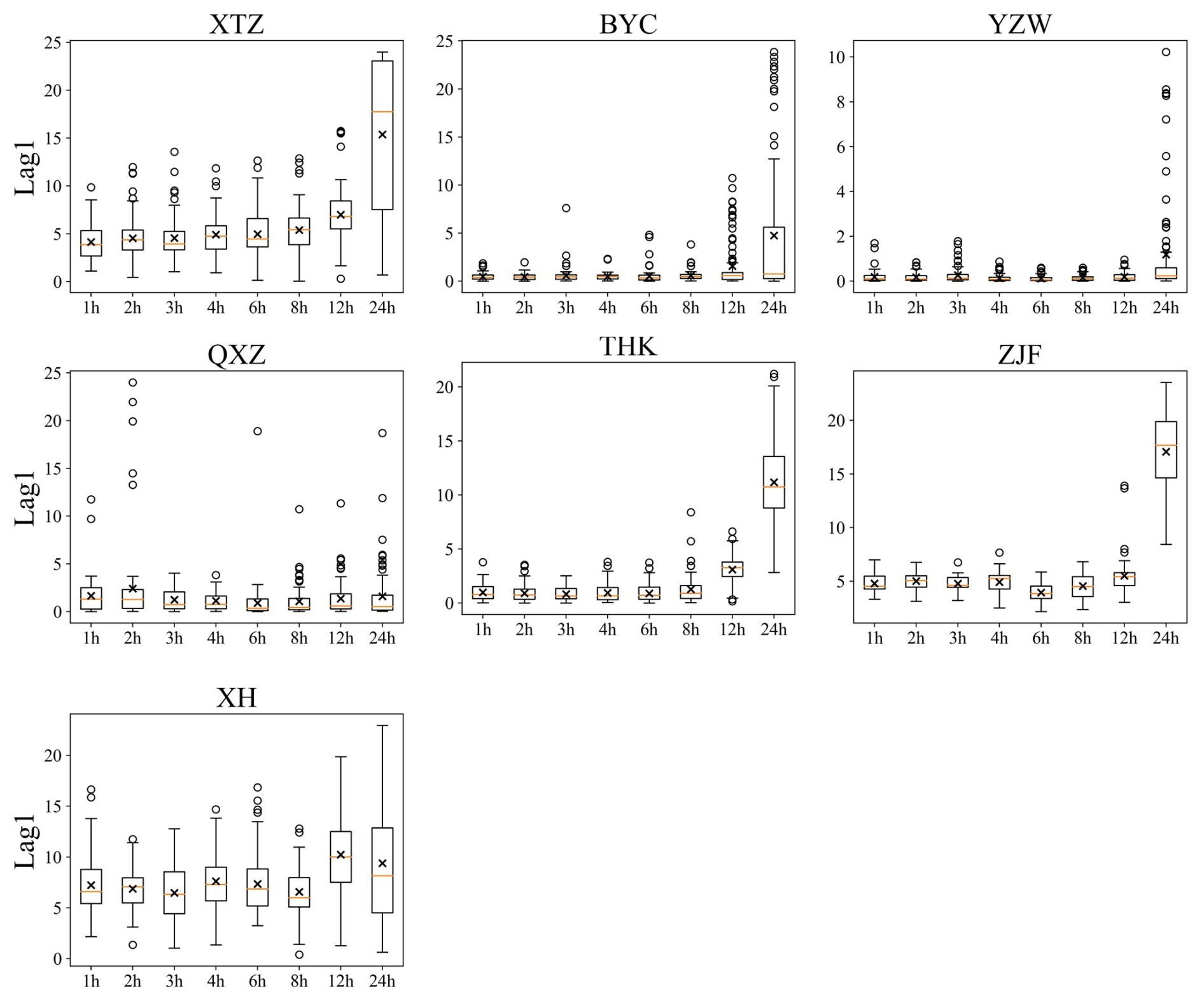
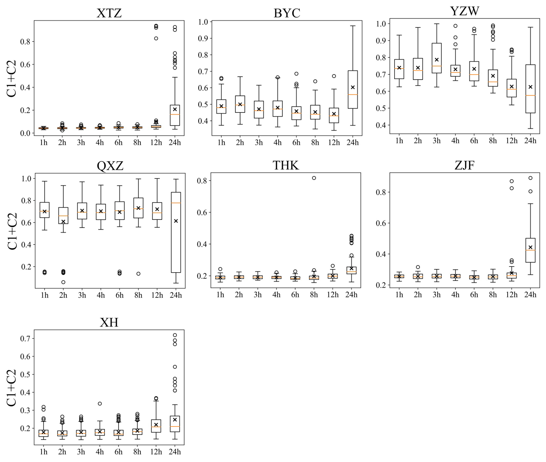
The results indicated that when the computational time step is fixed as 1 h, parameters calibrated under different data resolutions can be transferred and used in models with other resolutions. To further explain the transferability of parameters and identify any patterns as resolution changes, we compared parameters across different resolutions. However, due to the parameter equifinality (Her and Chaubey, 2015; Foulon and Rousseau, 2018), a single optimal parameter set may not be representative enough to accurately reflect the patterns. Therefore, we analyzed 100 sets of parameters calibrated at each resolution, with partial results shown in Figs. 10–12. The findings revealed that most parameters did not exhibit a significant and consistent trend of variation with changes in resolution. In other words, parameters calibrated under different resolutions showed little variability, which explains their transferability across resolutions. However, some parameters did show a certain consistent trend with resolution changes. Figure 10 illustrates the trend of the parameter Lag1 with changes in resolution. This parameter in the model reflects the lag time of surface runoff (the time from the generation of surface runoff until it reaches the outlet of the sub-basin). As the resolution becomes coarser (from 1 to 24 h), the effective information provided by the observed streamflow to the model decreases, and the requirement for precision in peak time also reduces in the calibration period. This relaxation in constraints led to an increase in both the mean value and the range of variation of Lag1. Notably, at stations XTZ, THK, and ZJF, when the data resolution is 24 h, the mean value of Lag1 exceeds 10 h or even 15 h, showing a significant difference from the value at 1 h resolution. The substantial divergence in the optimal parameters for models employing low-resolution versus high-resolution data results in a decline in model efficacy. This decline occurs even when high-resolution data is employed, provided that the parameters are those optimized for low-resolution data scenarios. In contrast, at stations BYC, YZW, and QXZ, when the data resolution is 24 h, the mean value of Lag1 is less than 5 h, which is not significantly different from the value at 1 h resolution. This provides an explanation for why NSE at XTZ, THK, and ZJF stations exhibits a decline when using high-resolution data, whereas other stations do not experience such a decrease.

Figure 10 Optimized values of Lag1 across various resolutions.

The parameter C₁+C₂ also exhibited a regular trend of variation with changes in resolution (Fig. 11). Generally, the larger this parameter, the faster the model's runoff responds to rainfall, resulting in a flood process that rises and falls sharply. When the time resolution is coarse, the variability of runoff may not be fully captured in the observed data. As a result, a model calibrated by coarser-resolution data tend to produce a smoother streamflow process. This is evident at stations such as YZW and QXZ, where the optimized C₁+C₂ value decreased as the resolution became coarser. However, we also observed that at most stations, including XTZ, THK, ZJF, and XH, this parameter increased as the resolution became coarser. This may be due to the model's computational time step of 1 h; when driven by coarse-resolution data, the input data are averaged over each hour, causing the runoff to be smoothed. Consequently, a larger C₁+C₂ value was selected by the parameter optimization algorithm to counterbalance this excessive smoothing.

Figure 11 Optimized values of C₁+C₂ across various resolutions.

Besides, in certain catchments, specific parameters exhibited regular changes across varying resolutions. At the BYC station, the parameter Ksg decreased as the resolution became coarser. Ksg represents the ratio of water transfer from the shallow subsurface layer to the deep groundwater layer. A decrease in Ksg would lead to the shallow subsurface layer becoming saturated more easily, resulting in more surface runoff. Similarly, at the YZW station, the parameter Kg decreased with coarser resolution. Kg represents the ratio of water conversion from the groundwater layer to groundwater runoff. A reduction in Kg would cause the groundwater layer to saturate more readily, also indirectly leading to increased surface runoff. The 1 h computational time step evenly distributes rainfall under coarse resolution, which reduces the simulated peak runoff compared to the actual peak. Therefore, the lower Ksg and Kg values improve simulation accuracy under coarse-resolution conditions by increasing surface runoff.

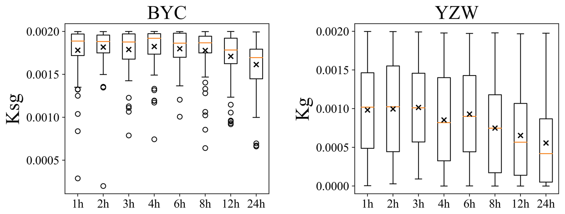
Figure 12 Optimized values of Ksg at BYC station and Kg in YZW station across various resolutions.

4.3 Parameters transferability across computational time steps

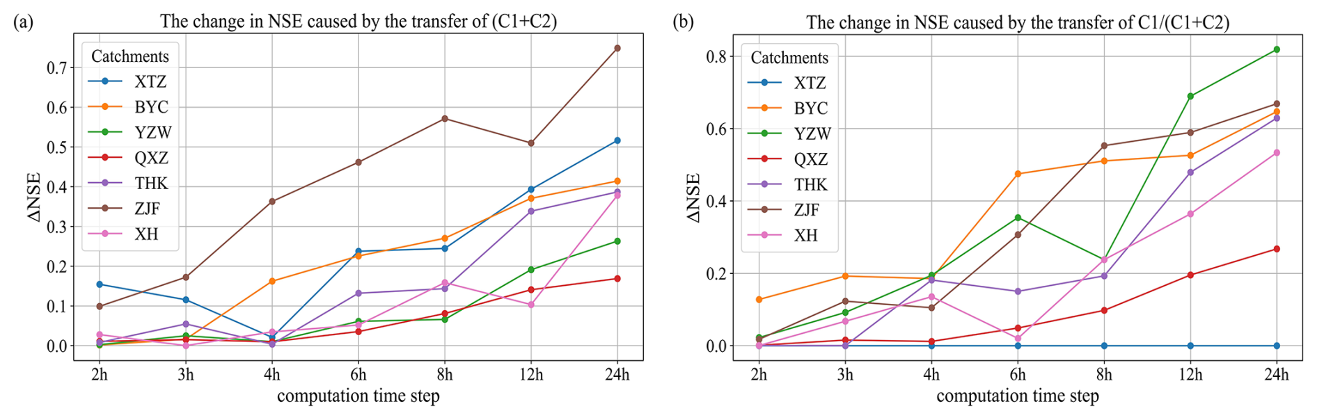
In contrast to the results of data resolution test, the findings from the computational time step test indicate that model parameters are not transferable across different computational time steps. To explain this non-transferability and identify the primary parameter responsible, we conducted the following test: each parameter from the optimal parameter set corresponding to ranging from 2 to 24 h time step was sequentially replaced with the optimal parameters for the time step of 1 h, and the change in NSE coefficient was observed when transferring only one parameter. Depending on the catchment and time step variations, the sensitive parameters causing significant changes in NSE differed; however, a common pattern emerged: in all catchments, two Muskingum parameters were consistently sensitive, and their influence varied systematically with the time step (as shown in Fig. 13). In the figure, ΔNSE represents the difference in NSE between using the optimal parameters for the respective time step and those transferred from the 1 h time step. As the distance between the source and destination time steps increases, the change in NSE caused by parameter transfer becomes more significant. In the XTZ catchment, NSE is influenced by C₁+C₂ rather than by $C_{\mathrm{1}}/(C_{\mathrm{1}}+C_{\mathrm{2}})$ because this catchment is very small and has not been subdivided into sub-catchments. It consists of only a single hydrological response unit, where the inflow in the routing process is solely lateral flow. By combining Figs. 7 and 13, it can be concluded that these two Muskingum parameters have a significant impact on model performance and are one of the main reasons for the non-transferability of model parameters across different computational time steps.

Figure 13 The change in NSE caused by the transfer of (a) C₁+C₂; (b) $C_{\mathrm{1}}/(C_{\mathrm{1}}+C_{\mathrm{2}})$.

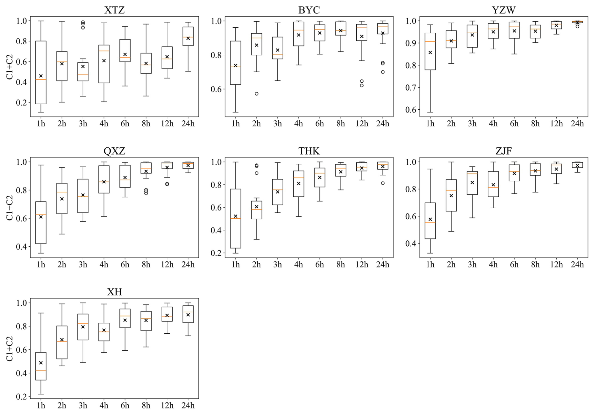
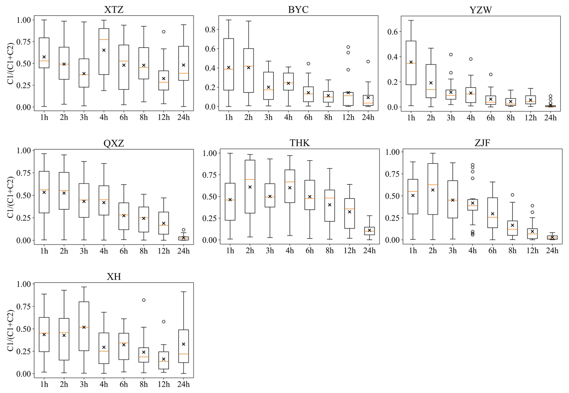
To further investigate the variation patterns of parameters with respect to model's computation time step, we analyzed the distribution characteristics of the top 20 best-performing parameter sets out of 100 optimal parameter sets. Unsurprisingly, the 2 Muskingum-related parameters exhibited clear variations with the change in the model's computation time step (as shown in Figs. 14 and 15). Specifically, C₁+C₂ increased as the time step grew (indicating that C₃ decreased, since the sum of the three parameters equals 1), suggesting that the weight of the inflow term in the routing process increases with the time step, while the correlation between the outlet flow at the end of the current time step ($Q_{\mathrm{i}}^{\mathrm{t}}$) and that at the end of the previous time step $(Q_{\mathrm{i}}^{t-\mathrm{1}}$) weakens. The value of $C_{\mathrm{1}}/(C_{\mathrm{1}}+C_{\mathrm{2}})$ decreased as the time step increased, implying that C₂ increased. This indicates that as the time step lengthens, the inflow from the upstream ($Q_{i-\mathrm{1}}^{\mathrm{t}}$) and the runoff generated within the current time step (Q_L) is more likely to be routed to the catchment outlet, enhancing the correlation between the outlet flow at the end of the current time step and the runoff produced within that time step. Furthermore, the variability in C₁+C₂ was notably greater than its variability across different data resolutions (as shown in Fig. 11), further confirming that its variability is one of the reasons for the non-transferability of parameters across different time steps. Figures 14 and 15 illustrate the variation patterns of the optimal Muskingum parameters for different computation time steps, which could serve as a reference for researchers and practitioners in the field of hydrological modeling.

Figure 14 Optimized values of C₁+C₂ across various computation time steps.

Figure 15 Optimized values of $C_{\mathrm{1}}/(C_{\mathrm{1}}+C_{\mathrm{2}})$ across various computation time steps.

4.4 Implications for the selection of data resolution and computation time step

The findings of this study offer several key insights for building hydrological models with limited data.

1. Data resolution considerations. For daily runoff simulations, it is found that a data resolution of 12 h is sufficient to provide accurate simulation results with relatively high precision. This suggests that higher-resolution data may not yield significant additional benefits for daily scale modeling. However, for hourly runoff simulations, the adequacy of data resolution depends on the specific objectives of the simulation. If the primary focus is on capturing the overall flood process, such as total runoff volume and approximate duration, 6 h resolution is adequate. On the other hand, if the simulation aims to achieve higher accuracy in peak flow estimation, employing data with finer temporal resolution can enhance the precision of these predictions. This offers practical insights for building numerical models and establishing monitoring stations, suggesting that high-resolution monitoring may not always be necessary. It is essential to balance the additional information gained from higher resolution against the associated costs, aligning with our objectives, enabling efficient resource allocation and ensuring that expenditures yield valuable returns.

2. Selection of computational time step. Regardless of whether the model is intended for daily or hourly runoff simulations and irrespective of the input data resolution, it is advisable to adopt a smaller computational time step when constructing the model. This is because the results show that the simulation accuracy on the coarse scale (24 h) with different computation time steps is almost the same, while the model running at a smaller computation step can produce results on a finer scale, which provides the possibility for further analysis. And the model's performance is particularly unreliable when parameters calibrated at larger computation time steps are transferred to smaller ones. This approach also ensures that the model parameters remain applicable across different data resolutions, thereby enhancing the model's flexibility and enabling it to generate accurate simulation results across a range of temporal scales. With the appropriate spatial scale and sufficient computational capacity, opting for a lower computational time step can make the model better equipped to maintain robust performance under varying input conditions and produce results at more timescales, which is crucial for ensuring the transferability of the model parameters and achieving consistent results.

5 Conclusions

5.1 Summary

This study assesses the value of different resolution data for daily and hourly streamflow simulations utilizing meteorological and runoff data with resolutions ranging from 1 to 24 h from 7 small- to medium-scale catchments in northern China. Additionally, the transferability of model parameters across varying data resolutions and computation time steps was investigated. Key findings are summarized as follows:

1. For both daily and hourly streamflow simulations, utilizing sub-daily resolution rainfall and streamflow data leads to substantial improvements in model performance compared with using the daily data. However, further enhancements in data resolution yield diminishing returns. Specifically, for daily streamflow simulations, improvements in model performance become negligible when the resolution exceeds 12 h. As for hourly streamflow simulations, improvements in overall flood process accuracy become negligible when the resolution exceeds 6 h, while higher resolutions further enhance the precision of peak flow predictions.

2. When the model's computation time step is fixed at 1 h, most parameters are generally independent of the input data resolution. Even when using model parameters obtained from daily data, utilizing sub-daily resolution data helps improve the accuracy of hourly streamflow simulations. Conversely, when the computation time step varies, the model parameters are not applicable for direct transfer to other time steps. In particular, the performance of the model deteriorates more when the computation time step is shifted from large to small.

3. It is recommended to utilize smaller computational time steps when constructing hydrological models even in the absence of high-resolution input data. This strategy ensures that the same prediction accuracy is achieved while preserving the transferability of model parameters, thus enhancing the robustness of the model.

5.2 Limitations and further research needs

While this study provides valuable insights into the impacts of data temporal resolution and computational time step on hydrological models, several limitations should be acknowledged. First, this study focuses on a specific geographical area in northern China and covers a limited temporal range. The findings, therefore, may not be fully generalizable to other regions with different climatic, hydrological, or geological conditions. Further studies across various regions and under different hydrological conditions are necessary to validate and extend the applicability of these results. Second, the study's conclusions are drawn based on a particular hydrological model and specific parameter settings. Other models or configurations might exhibit different sensitivities to data resolution and computational time step. Therefore, the generalization of these findings to other hydrological models should be approached with caution. Next, results show that the benefit of high-resolution rainfall/streamflow data to daily and hourly streamflow simulation was negligible when the temporal resolution was higher than a threshold, and the possible mechanism of such phenomenon is primarily discussed according to the variation of the runoff process and some parameters under different conditions and other existing literature. However, a deeper analysis and validation of such a threshold effect are still lacking, which needs further investigation. Last, the number of iterations for the optimization algorithm during the model calibration process was limited. Although our previous modeling and calibration practices (e.g., Nan and Tian, 2024a, b) demonstrated that the current number of iterations is sufficient to produce a good simulation, it does not guarantee the discovery of a globally optimal result. Consequently, it is challenging to determine whether the slight decline in model performance in certain catchments is due to the high-resolution data or the influence of local optima.