Technical note: How many models do we need to simulate hydrologic processes across large geographical domains?

Robust large-domain predictions of water availability and threats require models that work well across different basins in the model domain. It is currently common to express a model's accuracy through aggregated efficiency scores such as the Nash–Sutcliffe efficiency and Kling–Gupta efficiency (KGE), and these scores often form the basis to select among competing models. However, recent work has shown that such scores are subject to considerable sampling uncertainty: the exact selection of time steps used to calculate the scores can have large impacts on the scores obtained. Here we explicitly account for this sampling uncertainty to determine the number of models that are needed to simulate hydrologic processes across large spatial domains. Using a selection of 36 conceptual models and 559 basins, our results show that model equifinality, the fact that very different models can produce simulations with very similar accuracy, makes it very difficult to unambiguously select one model over another. If models were selected based on their validation KGE scores alone, almost every model would be selected as the best model in at least some basins. When sampling uncertainty is accounted for, this number drops to 4 models being needed to cover 95 % of investigated basins and 10 models being needed to cover all basins. We obtain similar conclusions for an objective function focused on low flows. These results suggest that, under the conditions typical of many current modelling studies, there is limited evidence that using a wide variety of different models leads to appreciable differences in simulation accuracy compared to using a smaller number of carefully chosen models.

1 Introduction

1.1 Model selection across large geographical domains

The need for robust predictions of water availability and threats across large spatial scales (i.e., national, continental, global) requires models that work well across a variety of landscapes, discretizations, and purposes. There are two main streams of thought on how this can be achieved. The first is the idea that a single model instantiation (i.e., a single set of equations that represent the whole spectrum of hydrologic processes with a single equation for each process) will be able to give accurate predictions everywhere and that the main challenges in large-domain modelling are related to our ability to parametrize, initialize, configure, and run models at ever finer resolutions (e.g., Freeze and Harlan, 1969; Wood et al., 2011; Bierkens et al., 2015; Arheimer et al., 2020). The second is the idea that there are limits to our ability to measure and model the real world, suggesting that the main challenges in large-domain modelling are related to our ability to select and parametrize appropriate models for different places under varying data availability (e.g., Kirchner, 2006; Clark et al., 2011, 2016, 2017; Addor and Melsen, 2019; Horton et al., 2022). This is sometimes referred to as the “uniqueness of place” (Beven, 2000) and in modelling terms suggests that one will need different models (i.e., different sets of equations) in different places depending on each location's dominant hydrologic processes. There is a need to reconcile both points of view and outline a path forward where the specific expertise of individuals and modelling groups can contribute to community efforts that advance our ability to predict hydrologic behaviour across large geographical domains.

The first paradigm of a single model structure has both strong appeal and strong theoretical and implementation challenges. The appeal of a single model structure is that (1) a single model suggests that we have complete understanding of how the system functions everywhere, all the time, and (2) implementing and maintaining a single model is much more tractable than doing so for multiple models. However, there are three distinct theoretical and implementation challenges that limit the applicability of prediction systems that rely on a single model structure across large geographical domains:

• First, our understanding of the equations that can be used to describe hydrologic behaviour is incomplete. We do not have a single set of equations that clearly and unambiguously describe hydrologic processes, process interactions, and scaling behaviour. Instead, we have many different equations for each process, and individual process parametrizations have their own assumptions, simplifications, and limitations.

• Second, despite a growing number of continentally or globally applied hydrologic models, we so far do not have a single model that contains an appropriate representation of the different hydrologic landscapes that manifest across continental domains. A rough north-to-south overview of the North American continent, for example, suggests that a model may need at least some ability to represent glaciers, permafrost, lateral snow distribution through wind and avalanches, (boreal) wetlands, surface depressions, agriculture, urban hydrology, aquifer recharge and abstraction, reservoir operation and water allocation, losing streams, fog interception, and multi-story canopies. Models that simulate a number of these processes exist, with the relevant expertise about different processes scattered across different individuals and groups.

• Third, the heterogeneity of the landscape combined with the often limited physiographic data available complicates model configuration, parametrization, and initialization. A model's appropriate horizontal resolution and process complexity may vary in space depending on data availability.

An alternative paradigm is the “multi-model mosaic” approach (e.g., Ogden et al., 2021; Johnson et al., 2023), where different models are selected for different regions based on each model's strengths and weaknesses. Instead of attempting to run a single model everywhere, the multi-model mosaic paradigm approaches the problem in a piecemeal fashion: use different models in different places, while ensuring that whatever model is chosen for a given place captures at least the dominant processes in that location. For example, glacier models are necessities for hydrologic modelling in the Canadian Rocky Mountains or the Himalayas but may be of limited added value for modelling across most of the low- and mid-latitude regions. Similarly, accounting for tile drainage and anthropogenic infrastructure is critical in agricultural and urban regions but of limited relevance for the sparsely populated high-latitude permafrost regions. The multi-model mosaic paradigm has practical appeal if it is able to deliver robust and actionable predictions with local relevance, at a reasonable computational cost.

The key challenge within such a paradigm is to select which model should be used for a given location. We can distinguish between two main approaches, each with their own challenges:

• First, it is possible to use detailed understanding of a specific place to refine perceptual models of that location's hydrologic behaviour (e.g., McGlynn et al., 2002) and from such understanding derive models that strike an appropriate balance between realism and accuracy of the resulting simulations (e.g., Kirchner, 2006; Fenicia et al., 2008, 2016). However, despite encouraging progress on synthesis efforts of perceptual models used by hydrologists (McMillan et al., 2023), we currently lack a detailed understanding of how the spatial variability in the drivers of hydrologic behaviour (i.e., climate, topography, land cover, and subsurface properties) translates to the spatial variability of dominant hydrologic processes across large domains. This prevents the use of these model development approaches for geographical domains much larger than individual research basins.

• Second, it is possible to rely on existing models and investigate how well such models perform for a wide variety of basins. This is especially attractive in the case of large geographical domains, where constructing new models for each location may be infeasible. Such approaches include model intercomparison projects (e.g., De Boer-Euser et al., 2017; Bouaziz et al., 2021; Mai et al., 2022b), investigations into model structure uncertainty (e.g., Lane et al., 2019; Knoben et al., 2020), and attempts to automatically calibrate model structures (e.g., Spieler et al., 2020; Mai et al., 2022a; Spieler and Schütze, 2024). One common challenge such studies have faced is that it has been difficult to relate model performance to model realism, and there is thus only limited guidance that would help select models that faithfully represent hydrologic behaviour for a given basin.

In many respects, the challenges with accuracy and process fidelity in the single-model paradigm have been replaced with new challenges of model structure identification in the multi-model paradigm.

In summary, despite the need for hydrologic predictions across large geographical domains (e.g., Eagleson, 1986; Beven, 2007; Bierkens, 2015; Blair et al., 2019), there is still limited understanding of which model or models would be appropriate to use for such large-domain predictions. Differences in the performance of different models are typically expressed through differences in metrics such as the Nash–Sutcliffe efficiency (NSE; Nash and Sutcliffe, 1970) or Kling–Gupta efficiency (KGE; Gupta et al., 2009). This is convenient when investigating model behaviour across many different locations, as would be the case in large-domain model performance assessments, but it is difficult to unambiguously select one model over another based on the aggregate NSE and KGE metrics alone. We will expand on this in the following section.

1.2 Equifinality during model identification

Studies that rely on aggregated performance metrics such as NSE and KGE need some way to account for equifinality (Beven, 1993, 2006; Beven and Freer, 2001; Ebel and Loague, 2006; Kelleher et al., 2017; Khatami et al., 2019): the concept that different simulations (resulting from different parameter sets for a given model or different models altogether) may obtain very similar or identical efficiency scores, as a consequence of reducing an entire time series of errors into a single number (Gupta et al., 2008).

Selecting models under equifinality may be done with Bayesian methods that estimate the likelihoods of different models or parameter sets (e.g., Vrugt et al., 2003, 2008; Kavetski et al., 2006a, b; Thyer et al., 2009; Renard et al., 2010; Schöniger et al., 2014; Höge et al., 2019). Two related alternatives to formal Bayesian approaches are ad hoc approaches that (1) consider any model that beats a given performance score threshold as a plausible candidate (e.g., the GLUE methodology, Beven and Binley, 1992; Beven and Freer, 2001; Krueger et al., 2010) or (2) quantify the number of models that perform within a given score difference from the best model in a given case (e.g., x models are within y KGE from the best model in a basin, Knoben et al., 2020; Spieler and Schütze, 2024). No matter if or how equifinality is accounted for, a brief overview of the literature shows that model structure equifinality tends to be high (e.g., Bell et al., 2001; Perrin et al., 2001; Clark et al., 2008; Seiller et al., 2012; Van Esse et al., 2013; De Boer-Euser et al., 2017; Lane et al., 2019; Knoben et al., 2020; Spieler et al., 2020; Bouaziz et al., 2021; Troin et al., 2022; Spieler and Schütze, 2024; Song et al., 2024). Taken together, these studies show there are distinct regional differences in model performance, and certain models may perform much worse for a given basin than other models, but it is typically possible to find multiple models that produce simulations with close-to-best performance for a given basin.

We specifically call out the results of two of these studies to provide context for the KGE scores discussed in later sections of this paper. First, Knoben et al. (2020) show that across a sample of 559 basins and 36 models, for the majority of these basins it is possible to find between 2 and up to 28 model structures that perform within Δ0.05 KGE from the best model in each basin. Second, Spieler and Schütze (2024) performed an extensive model structure identification exercise using close to 7500 automatically defined model structures, as well as 45 literature-based models. They found that for 12 climatically varied MOPEX catchments (Duan et al., 2006), at least 378 and up to 2100 of the tested model structures can perform within Δ0.05 KGE from the best model in each basin, though these models do so through very different internal dynamics. To summarize, findings about model structure identification based on aggregated performance metrics are mostly consistent: for most basins it is possible to obtain very similar system-scale performance with very different models. Under such conditions it is difficult to select the most realistic model out of competing alternatives with similar performance levels (Kirchner, 2006).

There have been suggestions in the literature that equifinality in model performance may be even larger than current understanding indicates. For example, Clark et al. (2008) show that for a specific basin, only 10 out of approximately 4000 time steps contribute some 70 % of the total model error (or, in other words, that 70 % of the total model error is concentrated in 0.25 % of the time steps). Similarly, in a study of 671 basins across the contiguous United States, Newman et al. (2015) show that in a large number of basins a period of less than 20 d out of a 15-year validation period contributes 50 % of the total error. This suggests a strong sensitivity of the chosen performance metric to the exact sample of days for which the metric is calculated. Recent work refers to this concept as “sampling uncertainty” in objective function values and provides methods to estimate the true value of system-scale performance metrics and quantify this uncertainty (Lamontagne et al., 2020; Clark et al., 2021). Building on the work of Lamontagne et al. (2020), Clark et al. (2021) introduce a bootstrap-jackknife-based strategy to quantify the sampling uncertainty for a given data period and use the same sample of 671 basins (Newman et al., 2015) to show that there is strong spatial variability in the sampling uncertainty inherent in aggregated efficiency scores. They also show that as a consequence of sampling uncertainty, for the majority of these basins tolerance intervals around NSE and KGE scores are larger than 0.10 NSE or KGE “points”, far exceeding the kind of score differences that are often seen as meaningful in other studies. However, explicitly accounting for the sampling uncertainty inherent in aggregated model performance scores is not (yet) common practice, and it is unknown to what extent sampling uncertainty affects attempts at model selection across large geographical domains.

1.3 Problem statement

In this technical note we revisit the model comparison study of Knoben et al. (2020), who calibrate 36 different lumped conceptual models for 559 basins across the contiguous United States. We specifically account for the sampling uncertainty in the KGE scores of these modelling results to answer three questions relevant within a multi-model mosaic paradigm. In the remainder of this section and the paper, we rely on the following definitions:

• Unless otherwise specified, best model for a given basin refers to the model with the highest performance score during model validation. Here, that performance score is the KGE.

• Uncertainty bounds, (sampling) uncertainty interval and related terms refer to the 5th to 95th objective function sampling uncertainty interval calculated for the best model (details on how this is done can be found in Sect. 2).

• Performance-equivalent and related phrases refer to any model with a validation KGE score that is within the uncertainty bounds of the best model in a given basin. In other words, performance equivalence is meant to indicate that when objective function sampling uncertainty is considered, two models are effectively indistinguishable in terms of their performance scores because one score falls within the uncertainty interval of the other.

These definitions of sampling uncertainty may not be intuitive. In an effort to enhance clarity, we therefore phrased each research question twice using different combinations of the definitions listed above:

1. For a given model, in how many basins does that model's performance score fall within the uncertainty bounds of the best model in that basin? Phrased differently, in how many basins is each model performance-equivalent with the best model in that basin?

2. For a given basin, how many models show performance scores within the uncertainty bounds of the best model in that basin? Phrased differently, how many models are performance-equivalent in each basin?

3. What is the minimum number of models needed to obtain simulations with performance that is within the sampling uncertainty interval of the best model in each basin? Phrased differently, what is the minimum number of models needed to obtain performance-equivalent simulations across the full domain?

Despite increasing attention for model structure uncertainty, and improved understanding of which models work well in different locations, selecting appropriate model structures across large geographical domains is an open challenge, and actual implementations of a multi-model mosaic paradigm for hydrologic prediction are still rare. Our aim with this paper is to highlight a core challenge such implementations will need to overcome in order to fulfil their goal of providing locally relevant, realistic, and optimally performant simulations. We focus our analysis on streamflow simulations only, but the concepts discussed in this work could be applied more broadly to hydrologic model evaluation.

2 Data and methods

2.1 Streamflow observations and simulations

We obtained streamflow observations, gauge locations and basin areas from the CAMELS data set (Newman et al., 2015; Addor et al., 2017b), and the model simulations for these basins described in Knoben et al. (2020). Briefly, Knoben et al. (2020) first select 559 out of the 671 basins provided in the CAMELS data set based on water balance closure considerations and estimated basin area errors. Next, the data for the remaining 559 basins are divided into two 10-year periods for model calibration and validation respectively. A total of 36 models taken from the Modular Rainfall Runoff Modelling Toolbox (MARRMoT; Knoben et al., 2019b) are then calibrated using the Kling–Gupta efficiency (KGE) as the objective function and streamflow as the variable of interest. The 36 models mimic existing published models such as IHACRES (Littlewood et al., 1997), TOPMODEL (Beven and Kirkby, 1979), and HBV-96 (Lindström et al., 1997) and thus cover a wide range of configurations, varying from a simple 1 store (i.e., state variable), 1 parameter bucket model to relatively complex configurations with up to 6 stores and 15 parameters. Of these models, 8 include a snow module, while the remaining 28 models have no real capability to deal with snow accumulation and snowmelt. We refer the reader to Knoben et al. (2019b) and Knoben et al. (2020) for further details about the toolbox and the specific model ensemble used here.

2.2 Methodology

Our analysis consists of four concrete steps (see also Fig. 1 for more details on steps 2 and 3 below):

1. The data package provided by Knoben et al. (2020) contains calibrated simulations for 36 models but does not include streamflow observations, and we therefore need to obtain these from the CAMELS data set (Newman et al., 2014; Addor et al., 2017a). We converted these observations from ft³ s⁻¹ into mm d⁻¹ using the GAGES II areas provided as part of the CAMELS data to match the simulations.

2. Using the observations and model simulations, we can calculate the KGE scores and quantify their associated uncertainty with the gumboot package (Clark and Shook, 2021; Clark et al., 2021). Briefly, gumboot returns various statistics, such as the 5th, 50th, and 95th percentile estimates of the KGE score through a “non-overlapping block” bootstrapping method that creates a sample of water years based on the data period provided. Each bootstrapped realization is based on random sampling with replacement of water years in the data period. Using water years as the non-overlapping blocks in the bootstrap ensures that each bootstrapped realization consists of hydrologically independent sub-periods. We use gumboot's default settings, such as those determined by Clark et al. (2021). This creates 1000 bootstrapped realizations, with October as the first month of the water year, and a water year must contain at least 100 valid (larger than 0) flow values. For simplicity, we only calculate the KGE uncertainty bounds for the best model (i.e., the model with the highest validation KGE score) in each basin and use these bounds to inform our analysis. We can use gumboot in 555 out of 559 basins. The remaining four basins contain years with no observed flow, and this interferes with the computation of standard deviations and correlations during gumboot's bootstrapping procedure. These four basins are excluded from further analysis. For the remainder of basins, we exclude all models with efficiency scores below the 5th percentile estimate of the KGE score of the best model in a given basin from further analysis and thus only keep those models with efficiency scores that fall within the uncertainty bounds of the best model in each basin.

3. The sampling uncertainty obtained from gumboot provides enough information to answer the first two research questions. To answer the third research question, we need to identify the minimum number of models needed to get performance-equivalent simulations in each basin. One way to find this minimum combination of models is to iteratively trial every possible combination of models and identify the first combination of models for which we obtain performance-equivalent simulations in all basins. Such a brute-force approach is guaranteed to be accurate but slow and proved infeasible for this work. A faster way is to rewrite the problem as a linear programming problem, where the goal is to find the minimum number of subsets needed to provide coverage for the full set. In our case, we have 36 subsets (one for each model) where each subset contains the basin identifiers where a given model is performance-equivalent with the best model. The full set contains the identifiers for all 559 basins, and the optimizer is tasked with finding the smallest number of subsets (i.e., models) needed to cover the full set (i.e., all basins). We refer the reader to our GitHub repository for further implementation details (Knoben, 2024).

4. To investigate the impact of the choice of objective function on these findings, we repeat steps (2) and (3) using the low-flow calibration results of Knoben et al. (2020). These rely on the same models and basins but use the reciprocal of flows to calculate model performance as KGE($\mathrm{1}/Q$). To avoid issues with zero flows, a constant ϵ equal to 1 % of mean observed flows is added on every time step to the observed and simulated flows (Pushpalatha et al., 2012; Knoben et al., 2020).

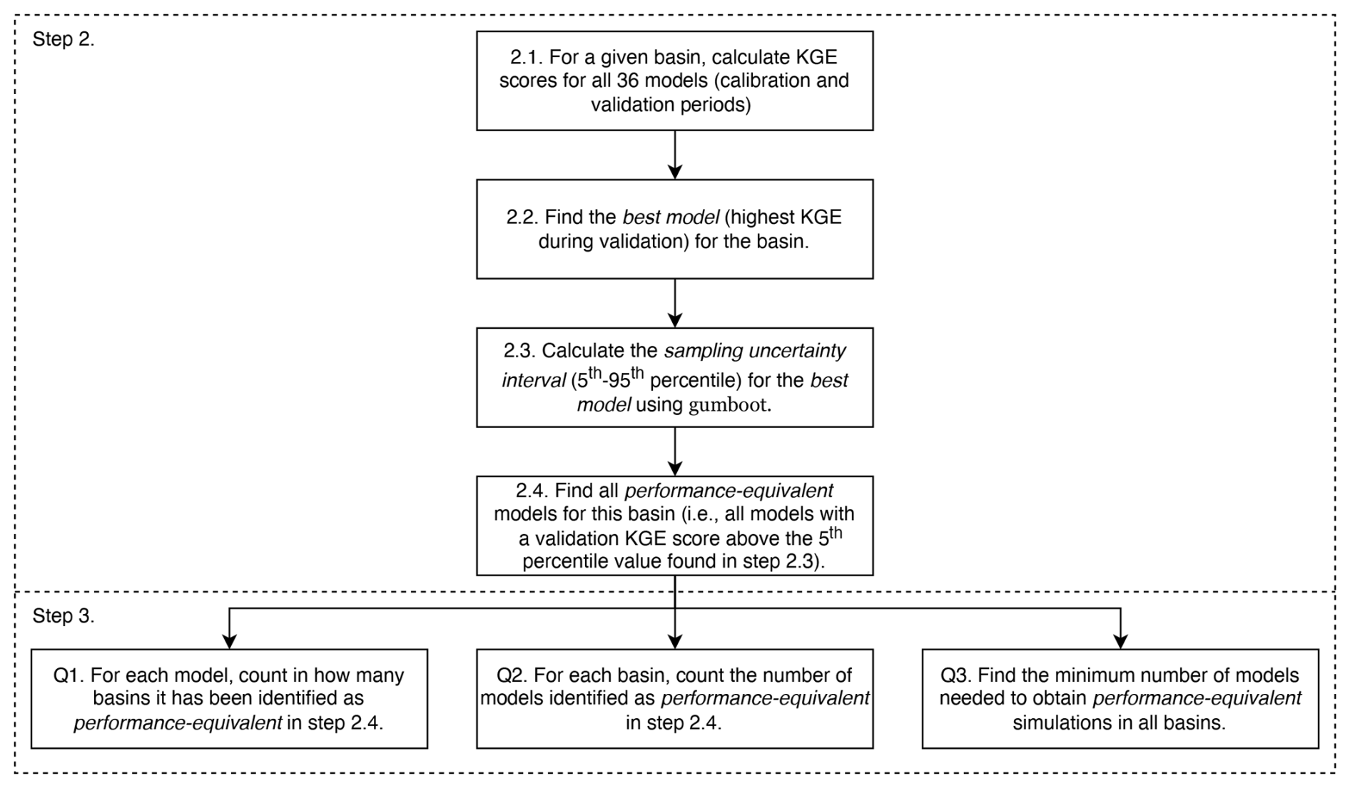
Figure 1 Description of steps 2 and 3 of the methodology used in this paper. Words in italics refer to the definitions provided in Sect. 1.3.

To aid in understanding the methods used here, Fig. 2 illustrates the sampling uncertainty and model filtering described in step 2 for the basin with the lowest (Fig. 2a and b) and highest (Fig. 2c and d) sampling uncertainty respectively. Figure 2a shows the observations and simulations in a basin with a strongly seasonal and relatively regular flow regime. KGE scores in this basin (Fig. 2b) are comparatively high, but the sampling uncertainty is low due to the regularity of the flow regime: the choice of data on which the best model is evaluated does not substantially change the KGE scores obtained for this model. Consequently, only a handful of models fall within the uncertainty bounds of the best model (grey horizontal lines), despite the overall rather high KGE scores obtained by all models (note the values on the y axis). In contrast, Fig. 2c shows observations and simulations in a basin dominated by irregular high flow events. Despite the lower KGE scores obtained by all models (Fig. 2d; note different y axis compared to Fig. 2b), the sampling uncertainty around the score of the best model is so large that all models are within the uncertainty bounds of the best model for this basin. This basin is a prime example of a location where individual events/time steps have a disproportionate effect on the overall KGE score, and the exact data sample chosen to be used in validation of the models thus has a large impact on which scores are obtained.

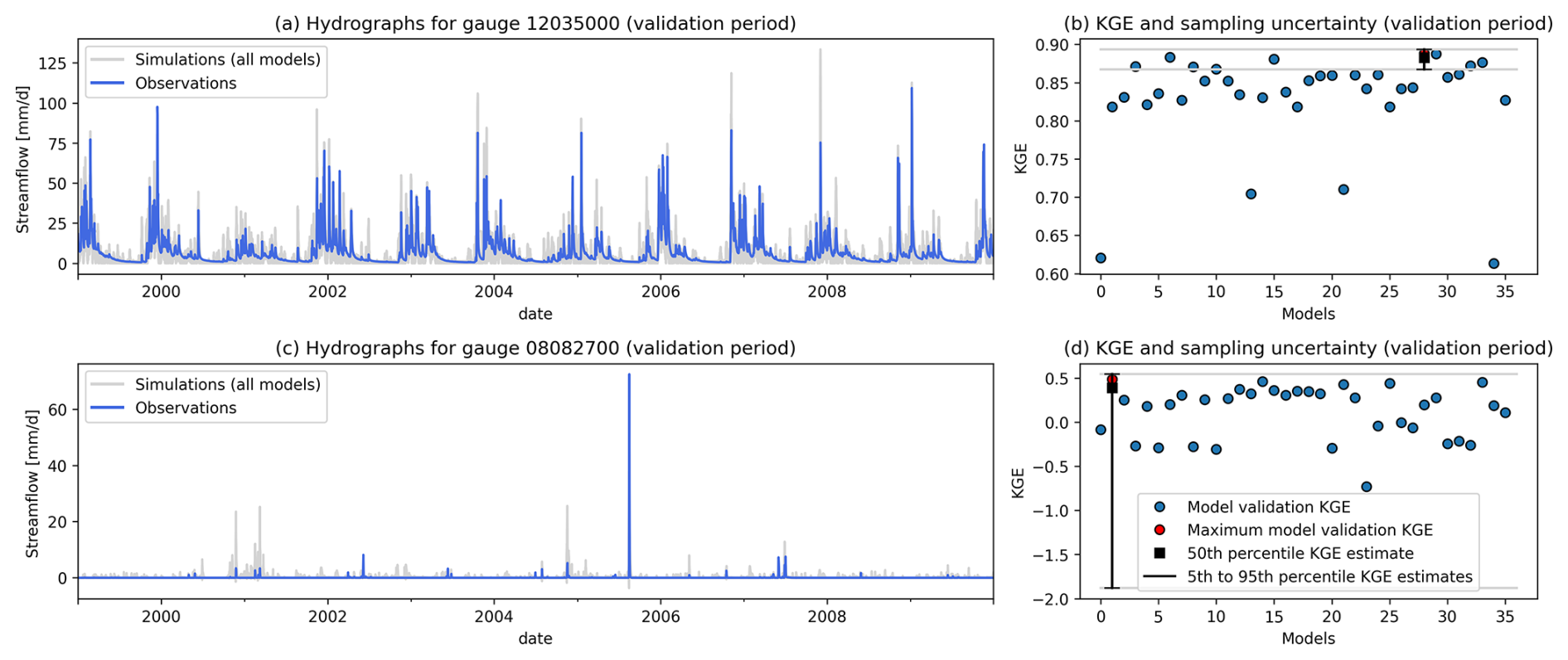
Figure 2 Example basins to illustrate the methodology. (a) Observations and simulations for the gauge with the lowest KGE sampling uncertainty within the 555 tested basins (USGS 12035000; Satsop River near Satsop, Washington). (b) Model scores during validation, as well as sampling uncertainty ranges for the best model for basin 12035000. Grey lines show how the uncertainty range compares to each individual model's KGE score. (c) Observations and simulations for the gauge with the highest KGE sampling uncertainty within the 555 tested basins (USGS 08082700; Millers Creek near Munday, Texas). (d) Model scores during validation, as well as sampling uncertainty ranges for the best model for basin 08082700. Grey lines show how the uncertainty range compares to each individual model's KGE score.

3 Results

3.1 Objective function values and sampling uncertainty

Figure 3 shows (a and d) the maximum KGE score found for each basin, (c and d) the uncertainty associated with these scores (here expressed as the difference between the 95th and 5th percentile estimate of the KGE score estimated by gumboot), and (b) the model from which the maximum KGE is obtained in each basin. These results are in line with earlier reports on regional differences in model performance (see, e.g., Newman et al., 2015; Knoben et al., 2020), uncertainty in model performance scores (see, e.g., Newman et al., 2015; Clark et al., 2021), and the considerable scatter in which model would be chosen based on maximum performance alone (see, e.g., Perrin et al., 2001; Knoben et al., 2020). We included these results here to provide context for the remainder of this section.

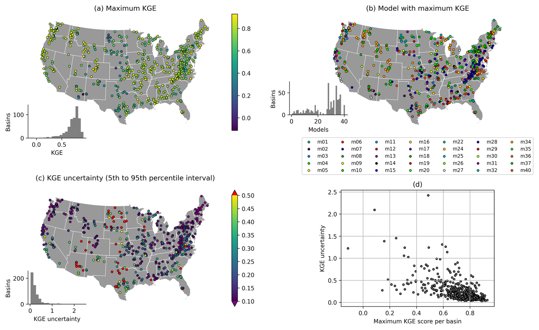
Figure 3 Model results for 555 CAMELS basins. (a) Maximum KGE score obtained per basin for the evaluation period. (b) Model that obtains the maximum evaluation KGE score shown in (a). (c) Sampling uncertainty in KGE scores obtained from gumboot, with the colour axis capped at either end for clarity. (d) Scatter plot showing the relation between the KGE of the best model in each basin and its associated uncertainty interval. Borders obtained from Commission for Environmental Cooperation (CEC) (2022).

3.2 Equifinality as a consequence of objective function sampling uncertainty

Figure 4a shows the number of basins in which each model achieves a performance score that falls with the uncertainty bounds of the best model for each respective basin or, in other words, the number of basins for which a model is performance-equivalent with the best model in a given basin. The MARRMoT toolbox contains a wide range of different model structures, and even the worst of these is performance-equivalent to the best model in at least 50 basins (i.e., slightly below 10 % of cases, while this model, m01, already was the top-performing model in only in a handful of these basins – see the histogram inset in Fig. 3b). The model that is performance-equivalent to the best model in the most basins is one of medium complexity (m28, 4 state variables, 12 parameters) and performs within the uncertainty bounds of the best model in 362 basins (i.e., almost two-thirds of cases; the model was already the top-performing model in slightly over 70 of these basins – see Fig. 3b). Critically, this model does not include a snow routine. The calibration procedure will have tried to compensate for this lack through parameter optimization, but it is unlikely for this model to perform well in any basin that experiences a substantial amount of snowfall.

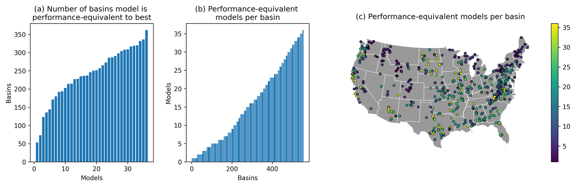
Figure 4 (a) Number of times each model falls within the uncertainty bounds around the performance of the best model in each basin. Note that a model can fall within its own uncertainty bounds. Models are ordered by number of basins, not by their MARRMoT IDs. (b) Number of models that fall within the uncertainty bounds around the best model's performance for each basin. (c) Spatial overview of (b). Borders obtained from Commission for Environmental Cooperation (CEC) (2022).

Figure 4b shows that the number of performance-equivalent models varies strongly between basins, and Fig. 4c shows this information across space. There are a handful of basins where the number of performance-equivalent models is modest, but for most basins it is possible to find numerous models that are within the uncertainty bounds of the best model. In fact, in 7 basins (approximately 1.5 % of all cases) every single model in the ensemble obtains validation KGE scores that are within the uncertainty bounds of the best model. Figure 4c shows only one obvious regional signal, which is an artifact of the experimental design. Only eight of the tested model structures include a snow routine, and regions that experience more snowfall (i.e., the Rocky, Cascade, and Sierra Nevada mountain ranges, as well as the Northeast and the Great Lakes regions, Addor et al., 2017b) thus have lower numbers of performance-equivalent models. Across the remainder of the domain where snow plays a smaller role, no clear patterns in the number of performance-equivalent models exist.

3.3 Model selection under objective function sampling uncertainty

Figure 5 shows the outcome of our model selection procedure, where we try to minimize the number of models needed to obtain performance-equivalent simulations in all basins. As shown in Fig. 5a, a single model (m28 in MARRMoT identifiers) is performance-equivalent to the best model in almost two-thirds of the basins, and only four models (m28, m34, m37, m36) are needed to get performance equivalence in more than 95 % of basins. An initial exploration of mapping model structures onto hydroclimates suggests that this first model (4 state variables, 12 parameters) achieves performance equivalence in a wide variety of hydroclimates, which may be due to its flexible treatment of variable contributing areas. The next two models (m34, 5 state variables and 12 parameters, and m37, 5 state variables and 15 parameters) perform well in snow-dominated basins, due to their snow accumulation and melt routines. The first of these has a basic degree-day snow model coupled to a model structure that incorporates two parallel unit hydrographs. This may give the model a certain capability to simulate heterogeneity in basin runoff as a consequence of spatial differences in snowmelt timing. The second contains a more complex snow accumulation and melt routine that has the capability to refreeze meltwater, which may provide some capability to deal with the consequences of intermittent melt events during winter. The distinguishing feature of the fourth model (m36; 5 state variables, 15 parameters) is its ability to represent losing streams, though it is difficult to determine to what extent this plays a role here. Another six models are needed to fill the remaining 21 basins, at 8, 5, 4, 2, 1, and 1 basin(s) respectively. We consider these numbers small enough to be noise, likely caused by data and parameter uncertainty.

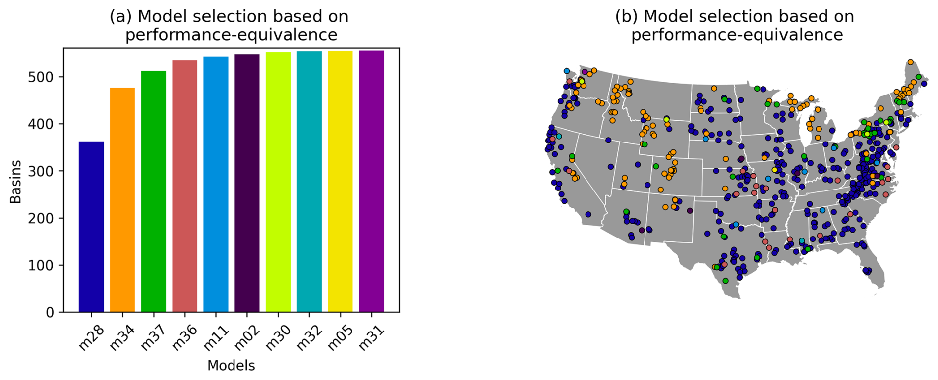
Figure 5 Outcome of model selection for large-domain modelling. (a) Number of basins covered by an increasing number of models. mxx refers to the model identifier. (b) Spatial distribution of basins covered by each model (colours refer to specific models as shown in a). Borders obtained from Commission for Environmental Cooperation (CEC) (2022).

3.4 Objective function impact

Figure 6 repeats the earlier analysis with model simulations obtained when calibrating the models to a KGE($\mathrm{1}/Q$) target. This is intended to emphasize low flows and leads to considerable differences compared to the findings based on KGE(Q), though the context of the problem remains the same: there are certain spatial differences in the maximum KGE scores obtained (Fig. 6a), and model selection based on these maximum KGE scores would lead to a patchwork of different models being used (Fig. 6b). Figure 6c shows that generally the models are performance-equivalent to the best model in fewer basins. In fact, the worst model is only performance-equivalent to the best model in a single basin (compared to 53 before), and the best model is performance-equivalent to the best model in 263 basins compared to 362 before. This is reflected in the number of performance-equivalent models in each basin (Fig. 6d and e), which shows a very different distribution for this objective function than before (compare with Fig. 4b and c). Consequently, almost double the number of models is needed to obtain close-to-best performance throughout the entire domain (Fig. 6f and g), with eight models being needed to obtain 95 % coverage. Critically, these models only partially overlap with the models identified in Fig. 5. The findings presented in this paper are thus conditional on the chosen objective function, but, compared to the “almost every model is the best somewhere” model selection case visible in Fig. 6b, the general message holds: if one accounts for the sampling uncertainty in KGE scores, fewer models are needed to obtain performance-equivalent simulations than one might expect.

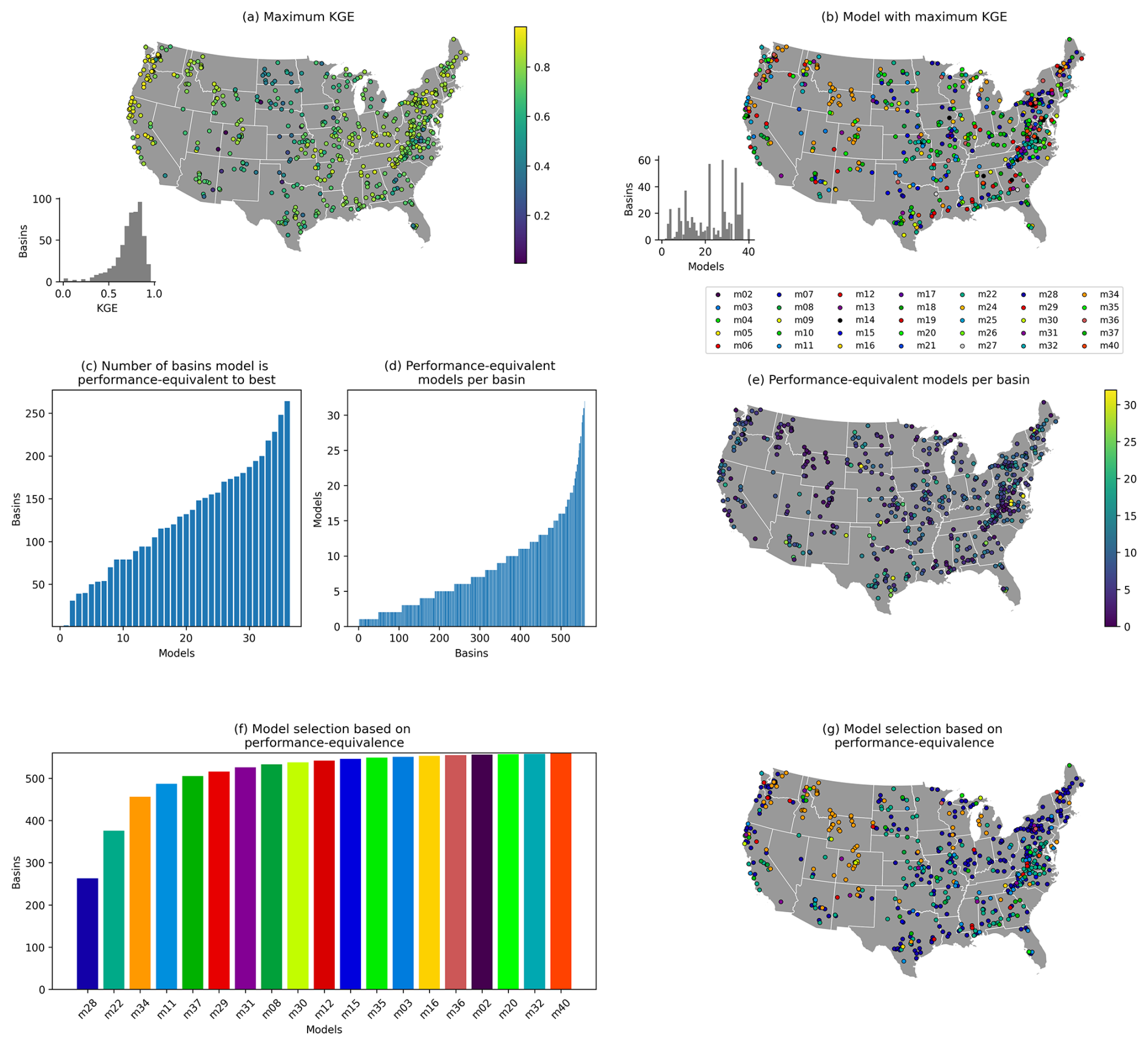
Figure 6 Repeat of earlier analysis for models calibrated with a KGE($\mathrm{1}/Q$) objective function. (a) Maximum KGE score per basin. (b) Model from which the maximum KGE score in each basin is obtained. (c) Number of times each model falls within the uncertainty bounds around the performance of the best model in each basin. Note that a model can fall within its own uncertainty bounds. (d) Number of models that fall within the uncertainty bounds around the best model's performance for each basin. (e) Spatial overview of (d). (f) Number of basins covered by an increasing number of models. mxx refers to the model identifier. (g) Spatial distribution of basins covered by each model (colours refer to specific models as shown in f). Borders obtained from Commission for Environmental Cooperation (CEC) (2022).

4 Discussion

The concept of equifinality has been discussed in the literature for a considerable time (Beven, 1993), and, given the existing literature on model structure uncertainty (e.g., Bell et al., 2001; Perrin et al., 2001; Clark et al., 2008; Krueger et al., 2010; Seiller et al., 2012; Van Esse et al., 2013; De Boer-Euser et al., 2017; Lane et al., 2019; Knoben et al., 2020; Spieler et al., 2020; Bouaziz et al., 2021; Troin et al., 2022; Spieler and Schütze, 2024), the results presented in this paper are not surprising. However, detailed understanding of the sampling uncertainty in performance metrics is a relatively recent development (e.g., Lamontagne et al., 2020; Clark et al., 2021), and accounting for sampling uncertainty in model comparison studies or during model selection is not yet common. We show in this paper that accounting for sampling uncertainty makes it very difficult to distinguish among competing models. It is possible to use performance scores to weed out extremely poor models, but the sampling uncertainty in these scores makes it difficult to meaningfully select appropriate model structures beyond the trivial (e.g., that a snow module is needed in basins with snowfall or that including some form of soil evaporation is helpful – see also Fig. 6 in Spieler and Schütze (2024) and the accompanying discussion therein).

This has various implications for large-domain model selection. Whereas uniqueness of place (Beven, 2000) suggests that different models will be applicable for different landscapes, there is so far only limited (mostly local, i.e., from single or small numbers of catchments) evidence that “uniqueness of models” leads to appreciable increases in model performance. Local studies in research basins typically have the benefit of more complete data availability, longer records, and extensive experience of the modeller with the basin in question (e.g., Fenicia et al., 2016), and this allows model evaluation and improvement until a model produces “the right results for the right reasons” (Kirchner, 2006). Across large geographical domains, aggregated objective scores currently remain the leading method for model selection and improvement, and our results suggest that in such methodologies a (very) small number of models will be sufficient to achieve close-to-best performance for most basins. In fact, given the high predictive power of machine learning approaches such as long short-term memory networks (LSTMs;  Kratzert et al., 2019; Klotz et al., 2022) and hybrid models (e.g., Shen et al., 2023; Song et al., 2024), it is distinctly possible, though yet unproven, that just a single model structure will be sufficient to achieve performance equivalence across such large domains. As evidenced by the different results we obtained for different objective functions, however, this comes with the caveat that such a model may not necessarily be appropriate for different purposes, and it may be that generalizing across geographical space is easier than finding a model that works well in different regions in objective function space.

Regardless, the concerns outlined by Kirchner (2006) still apply: high efficiency scores do not guarantee internally realistic models, and this may be of concern when those internal variables are needed for prediction of environmental hazards such as floods, droughts and wildfires. Possible paths forward for selecting models based on realism will likely need to at least partially mimic the approaches already applied at smaller scales. First, perceptual models of hydrologic behaviour that span large geographical domains are needed. Next, this understanding of hydrologic behaviour needs to be mapped onto models, modules, or specific equations that represent some (combination of) hydrologic process(es) correctly (for example, through hypothesis testing, Clark et al., 2011). Finally, diagnostic model evaluation approaches that go beyond aggregated error metrics are needed to quantify each models strengths and weaknesses (Gupta et al., 2008; Euser et al., 2013). Many of the elements required to apply these approaches to large geographical domains already exist, but synthesis efforts to bring these elements together are still rare. Concentrated community efforts will be needed to make progress on this topic.

5 Limitations and future work

5.1 Objective function distributions

We use a fairly simplistic approach to account for the sampling uncertainty in objective functions in this work, by only accounting for the sampling uncertainty of a single model in each basin. This has two theoretical limitations. First, we select the single model in each basin using the KGE scores obtained for the full validation period, without accounting for sampling uncertainty in this first selection. Preliminary analysis (not shown in this paper for brevity but accessible on the GitHub repository that contains the code used in our analysis) suggests that these full-period scores correlate with the estimated 50th percentile scores obtained with gumboot, but some scatter is present. Second, we do not account for the KGE sampling uncertainty for other models in each basin and simply rely on the KGE scores obtained for the full validation period to determine whether or not that model is considered within the sampling uncertainty of the best model in each basin. Practically speaking, one can envision a scenario where model X by chance barely falls within the uncertainty bounds of the best model Y, but that model X's own uncertainty interval mostly falls outside that of Y. In such a case it may not be the most sensible to treat model X and Y as performance-equivalent. Future work could account for the objective function sampling uncertainty in all models and use the fractional overlap of objective function distributions for analysis. Doing so would address both limitations at the same time. This would also open up the opportunity to investigate different definitions of the “best model for each basin”, such as selecting the best model as a compromise between its estimated 50th percentile KGE estimate and the size of the associated uncertainty interval.

5.2 Model selection

The models used in this work were a convenient choice but represent a subset of the wider range of hydrologic models available. Extending the sample by including different models of varying complexity (e.g., physics-based models and machine learning models) could provide valuable insights. Similarly, our sample of conceptual models is somewhat limited by the fact that only eight of these models have a dedicated snow component. The relative success of one of these “no-snow” models in representing hydrologic behaviour in a wide variety of basins (see Fig. 5a) strongly suggests that further investigations using conceptual models connected to snow routines will be worthwhile.

5.3 Modelling purpose

In this paper we investigated the number of models needed to reach full domain coverage for two different objective functions, under the assumption that these different objective functions are representative of different modelling goals. However, there are different ways to investigate the number of models needed for specific purposes. For example, follow-up work could investigate the stability of our conclusions for simulation of different flow percentiles, such as the lower 10th percentile for simulation of low flows and droughts or the upper 90th percentile for simulation of floods.

6 Conclusions

We investigated the number of conceptual models needed to obtain accurate simulations for 559 basins across the contiguous United States. The novelty of this work is that we explicitly account for the sampling uncertainty in the Kling Gupta efficiency (KGE) scores that we use to quantify the accuracy of each model's simulations. This sampling uncertainty refers to the fact that in certain basins individual time steps used to calculate scores such as KGE can have a disproportionate impact on the overall score. Consequently, the choice of calibration and validation periods can strongly impact the KGE scores obtained, and the same simulations may be valued very differently depending on how the calibration and validation data are chosen.

Accounting for this sampling uncertainty reveals that it is often very difficult to distinguish among competing models. If we were to select models based on their validation KGE scores only, almost all of the investigated 36 models would be selected for at least a handful of basins. When we account for the sampling uncertainty in the KGE scores, we find that every model is close to the performance of the best model (i.e., performance-equivalent) in at least 50 and up to 350+ basins (research question 1; Fig. 4a). Conversely, we find that in almost all basins at least 2 and up to all 36 models have similar performance (research question 2; Fig. 4b). Finally, when we account for the sampling uncertainty in the KGE scores, the number of models required to get performance-equivalent simulations on all basins drops drastically compared to selecting models based on the best KGE in each basin. Only four models are needed to get simulations with acceptable accuracy in 95 % of basins. With 10 models, 100 % coverage is obtained, without accounting for further complicating factors such as data and parameter uncertainty (research question 3; Fig. 5). These findings hold for a different objective function aimed at low-flow simulation: the KGE of the reciprocal of flows. Compared to almost all models being selected based on validation KGE($\mathrm{1}/Q$) scores, only 8 models are needed to cover 95 % of basins and 19 models for 100 % coverage (Fig. 6).

The results presented in this paper have consequences for model selection across large geographical domains. Whereas uniqueness of place suggests that different models will be applicable to different landscapes, the results of this analysis suggest that uniqueness of models does not necessarily lead to appreciable increases in model performance. Further work will need to show whether this is a general rule or if with more thoughtful model evaluation procedures the connection between models and places can be made more explicit. In the meantime, model selection procedures based on scores such as KGE will suggest that a small handful of models is adequate to simulate streamflow if the sampling uncertainty in such scores is explicitly accounted for.