Optimising ensemble streamflow predictions with bias correction and data assimilation techniques

This study evaluates the efficacy of bias correction (BC) and data assimilation (DA) techniques in refining hydrological model predictions. Both approaches are routinely used to enhance hydrological forecasts, yet there have been no studies that have systematically compared their utility. We focus on the application of these techniques to improve operational river flow forecasts in a diverse dataset of 316 catchments in the United Kingdom (UK), using the ensemble streamflow prediction (ESP) method applied to the (Génie Rural à 4 paramètres Journalier) (GR4J) hydrological model. This framework is used in operational seasonal forecasting, providing a suitable test bed for method application. Assessing the impacts of these two approaches on model performance and forecast skill, we find that BC yields substantial and generalised improvements by rectifying errors after simulation. Conversely, DA, adjusting model states at the start of the forecast period, provides more subtle enhancements, with the biggest effects seen at short lead times in catchments impacted by snow accumulation or melting processes in winter and spring and catchments with a high baseflow index (BFI) in summer. The choice between BC and DA involves trade-offs considering conceptual differences, computational demands, and uncertainty handling. Our findings emphasise the need for selective application based on specific scenarios and user requirements. This underscores the potential for developing a selective system (e.g. a decision tree) to refine forecasts effectively and deliver user-friendly hydrological predictions. While further work is required to enable implementation, this research contributes insights into the relative strengths and weaknesses of these forecast enhancement methods. These could find application in other forecasting systems, aiding the refinement of hydrological forecasts and meeting the demand for reliable information by end-users.

1 Introduction

Hydrological forecasts are a critical tool for water resource management, flood forecasting, and drought mitigation. In a warming world, we expect to see an increase in both high-flow and low-flow extremes, which will cause a wide range of impacts on society and the environment (Kreibich et al., 2022). Therefore, the need for reliable hydrological forecasts is more critical than ever, such that proactive action can be taken to mitigate these impacts.

There are different approaches to operational hydrological forecasting, ranging from process-based models to fully data-driven approaches. In the United Kingdom (UK), the Hydrological Outlook UK (HOUK) provides operational forecasts which are used by a range of stakeholders to support their decision-making (Hannaford et al., 2019). The HOUK uses three different approaches to produce its forecasts (Prudhomme et al., 2017). For the first approach, hydrological models are driven with seasonal weather forecasts produced by the UK Met Office (UKMO) to derive river flow forecasts (Bell et al., 2013). A second, dual approach, which is purely data-driven and based on statistical methods, generates “persistence” forecasts using flow anomalies in the most recent month and “historical analogue” forecasts using the most similar historical sequences (Svensson, 2016). The third approach, which is the one we are focusing on in this paper, is ensemble streamflow prediction (ESP), where a hydrological model is driven by an ensemble of historical climate time series to generate probabilistic streamflow forecasts (Harrigan et al., 2018). The operational ESP uses all available years of historical meteorological data from 1961 onwards to generate forecasts, i.e. currently the period 1961–2024. Each year, a new ensemble is added as more data become available. The initial hydrological conditions (IHCs) are calculated by driving the hydrological model (currently GR6J; previously GR4J until November 2023) with observed meteorological data from UKMO in near real time. These data include provisional, non-quality-controlled precipitation and temperature grids (HadUK; Hollis et al., 2019). Potential evapotranspiration (PET) is calculated using the calibrated McGuinness–Bordne equation as outlined by Tanguy et al. (2018).

Alternative approaches include long-term average scenarios, where catchment hydrological models are driven by rainfall scenarios assuming specific percentages of long-term average rainfall (e.g. 60 %, 80 %, or 100 %). This method is used in monthly water situation reports by the Environment Agency (e.g. Environment Agency, 2022). Additionally, emerging approaches like the use of storylines and large ensembles to explore plausible worst-case scenarios for upcoming months are gaining popularity in water resource management (e.g. Chan et al., 2024; Kay et al., 2024).

This study will focus on enhancing hydrological predictions using the ESP method, which has long been used worldwide and forms the basis for many operational seasonal forecasting systems (Wood et al., 2016). The UK provides a test bed for application given the existence of the operational HOUK, but the results of this study could resonate in many other settings. The ESP method, as utilised in this paper, employs historical sequences of climate data (precipitation and potential evapotranspiration) to drive hydrological models, generating a range of possible future streamflow conditions. The source of the forecasting skill of the ESP method is accurate estimation of the IHCs, which, depending on the model, can include antecedent stores of soil moisture, groundwater, snowpacks, and channel streamflow (Wood et al., 2016; Wood and Lettenmaier, 2008), rather than skilful atmospheric forecasts. ESP therefore offers an ideal environment for testing forecast enhancement techniques since it isolates the skill associated with IHCs from that stemming from accurate meteorological forcings. The IHCs can be detected up to a year in advance (Staudinger and Seibert, 2014), depending on the catchment characteristics. Harrigan et al. (2018) show that, in the UK, ESP is particularly skilful in catchments with a long “memory” due to its great groundwater influence. These catchments are concentrated in the south-east of the country, where ESP shows forecasting skill for lead times of up to 6 months. In the north-west of the country, however, the skill of ESP is limited. This part of the country is dominated by “flashy” fast-responding catchments with steeper orography and little groundwater storage where the IHCs have less predictive power, and it highlights the limitations of the ESP method. Despite its simplicity, ESP outperforms other hydrological forecasting approaches in many cases and remains a hard-to-beat reference in terms of both skill and value (Peñuela et al., 2020).

The ability of ESP to produce skilful forecasts, as with any model-based forecasting approach, is also inherently linked to the capability of the hydrological models used to produce accurate streamflow simulations. Streamflow simulations produced by hydrological models contain multiple sources of uncertainties, including the model structure, parameterisation, forcing data, and initial conditions (Renard et al., 2010).

The GR4J (Génie Rural à 4 paramètres Journalier)¹ hydrological model was used in this study and has been shown to reliably simulate the hydrology of a diverse set of catchments (Perrin et al., 2003), including the temporal transition between wet and dry periods (Broderick et al., 2016). Smith et al. (2019) demonstrated the good performance of the GR4J model over 303 UK catchments, enabling historic streamflow data reconstruction. However, GR4J is a simple lumped catchment with only four parameters: (i) a soil moisture accounting reservoir, (ii) a water exchange function, (iii) a non-linear routing store to represent baseflow, and (iv) rainfall-runoff time lags controlled by two-unit hydrographs. This simple model has the advantages of being very quick to run and being computationally inexpensive, which are essential criteria for an operational service, but it might not be able to capture the complexity of some of the hydrological systems, resulting in some biases, particularly towards the extremes.

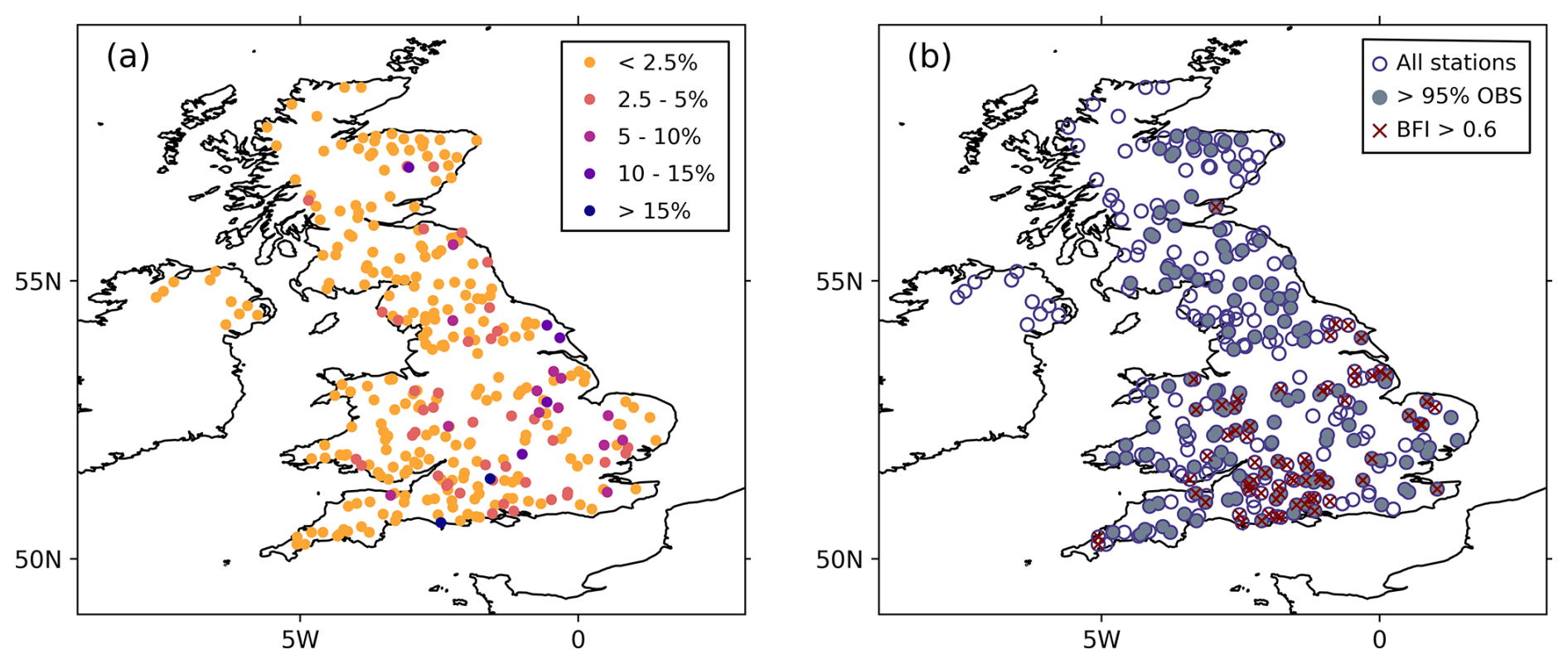
Figure 1 (a) Absolute percent bias (absPBIAS) in the 316 study catchments for streamflow simulated with the GR4J model, calculated based on the current analysis. (b) Locations of the gauging stations for the 316 NRFA catchments used in this study and their categories based on the amount of missing data and the value of the BFI.

While Lane et al. (2019) did not include GR4J in their study, they demonstrated a common challenge in hydrological modelling: systematic biases, which are particularly evident in regions with inadequate snowpack simulation, inter-catchment groundwater exchange, or significant human influence on the basin. Figure 1a illustrates the scale of the model bias for GR4J. Figures A4 and A5 show that the bias is generally greater for low flows when measured as a percent bias, whereas it is greater for high flows when considering raw bias values. To address this issue of hydrological model biases impacting predictions, researchers have developed various approaches to refining forecasts. Two prominent techniques are bias correction (BC; e.g. Bum Kim et al., 2021) and data assimilation (DA; e.g. Piazzi et al., 2021). While both methods share the common goal of enhancing forecast accuracy, they diverge fundamentally in their approaches. BC is a statistically based post-processing step that adjusts the forecast based on past performance, whereas DA improves the IHCs and corrects the internal model states. This fundamental difference may explain why there has been no prior attempt to compare the efficacy of these approaches in operational settings. However, from a user perspective, where the emphasis lies on the reliability of the final product to aid decision-making, such a comparison holds significant value. Ultimately, it can lead to the creation of more reliable end-products for users.

Several previous studies have shown the advantages of using BC as a post-processing technique to enhance the skill of hydrological forecasts (e.g. Chevuturi et al., 2023; Tiwari et al., 2022). Some operational systems, such as the GEOGloWS ECMWF Streamflow Service, apply BC to generate their forecasts (Sanchez Lozano et al., 2021). Hashino et al. (2007) conducted a study in which they compared various BC methods for ensemble streamflow forecasts and found that the quantile mapping (QM) method outperformed other techniques, resulting in a significant improvement in forecast skill. QM stands out as the most frequently employed approach in prior studies using bias correction to improve streamflow simulations (e.g. Chevuturi et al., 2023; Farmer et al., 2018; Usman et al., 2022). While some researchers opt to bias-correct precipitation and temperature prior to input into hydrological models, Tiwari et al. (2022) found that directly bias-correcting streamflow leads to superior results. Li et al. (2017) present a comprehensive review of forecast post-processing methods. QM stands out as one of the most popular options in hydrological forecasting due to its simplicity and efficiency (e.g. Hashino et al., 2007; Wood and Schaake, 2008). However, as an unconditional method, QM uses the cumulative distribution function (CDF) to perform the correction, and so it does not preserve the connection between each pair of simulated and observed values. Thus, QM may adjust the raw forecasts in the wrong direction for some forecast values (Madadgar et al., 2014). Note that, in our study, we apply QM BC using flow duration curves (FDCs) instead of CDFs. While statistically distinct, FDCs are better suited to hydrology due to their focus on flow exceedance probabilities. We view this as an extension of the QM framework tailored to hydrological data and have retained the term “quantile mapping” for consistency with the broader QM literature.

Unlike BC, which is applied as a post-processing step, the aim of DA is to improve the IHCs by combining models with observed data to improve the estimation of the target variable during the forecast period (e.g. Carrassi et al., 2018). In this way, DA can be seen as an effort to provide a more physically based improvement of the model predictions rather than as a statistically based post hoc correction. DA has a long history of application in meteorological (e.g. Navon, 2009) and hydrological (e.g. Liu et al., 2012) forecasting, but in the latter case it has tended to be focused on short lead times (typically of the order of days for flood forecasting applications; e.g. Piazzi et al., 2021). There have been relatively few studies of DA for sub-seasonal to seasonal forecasts in hydrology.

DA can be performed sequentially, using observed data as they become available, to update the model states and/or parameters. In this study, sequential DA of streamflow observations is performed during the model spin-up period to better approximate the IHCs at the start of the forecast period and to update the model parameter values. Previous research has demonstrated the potential of sequential DA approaches to improve model performance by reducing initial condition uncertainty (e.g. Piazzi et al., 2021). Two of the most popular methods are Kalman filters (e.g. Maxwell et al., 2018; Thiboult et al., 2016) and particle filters (e.g. DeChant and Moradkhani, 2011; Jin et al., 2013).

Kalman filter approaches for non-linear systems, such as the extended Kalman filter, are often limited by their high computational demand, unbounded error growth, and instability in the error covariance equation (Evensen, 1992). Ensemble Kalman filter (EnKf) approaches can be used to overcome some of these issues but rely on the assumption of Gaussian errors (Evensen, 1994). In contrast, particle filters do not make any assumptions regarding error distributions. However, particle filters may struggle in high-dimensional cases, requiring very large ensemble sizes to avoid “particle weight collapse”, where most particles end up with similar weights, failing to represent the full range of system states (Snyder et al., 2008).

For hydrological forecasts, Piazzi et al. (2021) show the potential effect of DA on skill improvement for a short lead time (2 d). Other work has shown that the impact of data assimilation and alternative approaches used to improve model skill, such as precipitation forcing, varies with lead times. However, the majority of the research in this area focuses on short- to medium-range forecasts (1–31 d lead times; e.g. Boucher et al., 2020; Clark et al., 2008; Piazzi et al., 2021; Randrianasolo et al., 2014; Seo et al., 2009; Sun et al., 2015; Thiboult et al., 2016). This is despite the improvements in hydrological forecasting making the production of skilful longer-term forecasts possible (e.g. Harrigan et al., 2018). Only a handful of studies have investigated the impact of initial condition estimates on longer lead times in hydrological forecasts in the United States (DeChant and Moradkhani, 2011; Shukla and Lettenmaier, 2011), showing generally improved seasonal predictions with DA but little added value beyond a 1-month forecast. However, beyond this, research into the potential of DA to improve seasonal and sub-seasonal hydrological forecast skill is limited. Therefore, there may be potential to improve skill at longer lead times by updating model parameters and initial streamflow states.

Note that other approaches, such as multi-model blending, have been used by others to improve forecasts (e.g. Chevuturi et al., 2023; Roy et al., 2020; Shamseldin, 1997) but will not be considered in this study.

The overall objective of this paper is to evaluate and compare the utility and effectiveness of the BC and DA approaches for optimising hydrological forecast outputs over a range of different lead times. This is achieved through application to a dataset of 316 UK catchments, representing a diverse range of catchment properties. We aim to provide guidance on the relative performance of these methods and how this varies according to location and catchment type, lead time, and time of year. As this is based on an operational seasonal forecasting product, i.e. the Hydrological Outlook UK ESP forecasts, it will enable users to make informed decisions and will provide insights into the most effective strategies for enhancing UK hydrological forecasting. More generally, these results can find application in other hydrological seasonal forecasting systems in other regions and can underpin future research in improving operational hydrological forecasts.

Table 1 Glossary of the abbreviations commonly used in this study.

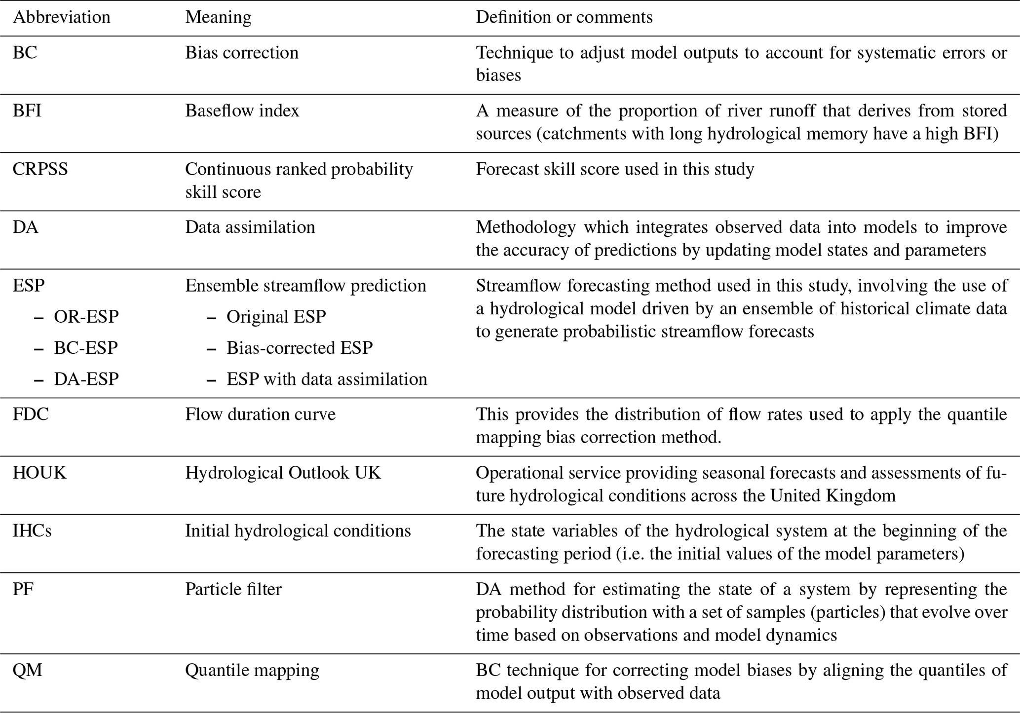
A glossary of the key abbreviations used in this study is provided in Table 1 for reference.

2 Material and methods

2.1 Data

2.1.1 River flow data

Observed daily river flow data were obtained for 316 catchments (Fig. 1) from the National River Flow Archive (NRFA, https://nrfa.ceh.ac.uk/, last access: 18 March 2025) database. For the full metadata of these catchments, see the Supplement of Harrigan et al. (2018). The catchment observations were used to calibrate the model (see Sect. 2.2), bias-correct the streamflow simulations (see Sect. 2.3), evaluate the model performance evaluation (see Sect. 2.5), and assess the forecast skill (see Sect. 2.6). The study period used was from 1 January 1961 to 31 December 2015.

For the forecast skill assessment, complete observed time series were needed (see Sect. 2.6), so gap-filling using simple linear interpolation was applied to the missing data in the observed river flow time series (the limitations of this method are discussed in Sect. 4.4). The gap-filled version of the dataset was only used for the forecast skill assessment, not for the other applications (model calibration, BC, and model performance evaluation).

Considering the amount of missing data in the observational dataset and the diverse hydrological characteristics of the catchments, we defined four different subsets of catchments (see Fig. 1b):

• i.

  The full set of catchments (316 catchments).

• ii.

  Catchments with less than 5 % missing observed river flow data (139 catchments).

• iii.

  Catchments with a BFI greater than 0.6 (70 catchments). The BFI is a measure of the proportion of the river runoff that derives from stored sources: the more permeable the rock, superficial deposits, and soils in a catchment, the higher the baseflow and the more sustained the river's flow during periods of dry weather (Gustard, 1992). In other words, the higher the BFI, the longer the catchment memory, and therefore improving the IHCs in these catchments has the potential to improve the hydrological forecasts for longer lead times.

• iv.

  Catchments with a BFI greater than 0.6 and missing observed river flow data of less than +5 % (29 catchments).

2.1.2 Meteorological data

To run the hydrological model (see Sect. 2.2), precipitation (P) and PET data are needed. For the P data, we used CEH-GEAR daily rainfall data (Keller et al., 2015; Tanguy et al., 2019). For the PET data, we used the CHESS-PET data (Robinson et al., 2017, 2020) for the UK and the Historic PET dataset (Tanguy et al., 2017) for Northern Ireland, where CHESS-PET is not available. Tanguy et al. (2018) describe how the Historic PET dataset was derived using a temperature-based PET equation calibrated using CHESS-PET. Consequently, these two datasets can be regarded as almost equivalent and sufficiently similar for our purposes. The meteorological data used also covered the period from 1961 to 2015.

2.2 Hydrological model, river flow simulations, and ESP hindcasts

2.2.1 Simulated observed river flows

The hydrological model used to simulate river flow was the GR4J model (Perrin et al., 2003), which served as the operational model for producing ESP forecasts in the HOUK until September 2023. The calibration approach adopted was consistent with Harrigan et al. (2018), where the modified Kling–Gupta efficiency (KGEmod; Gupta et al., 2009; Kling et al., 2012), applied to root-squared transformed flows (KGEmod[sqrt]), was used as the objective function for automatic fitting. This approach places weight evenly across the flow regime rather than focusing on high or low flows, a decision made considering that ESP forecasts are generated throughout the year, encompassing both dry and wet conditions.

Daily river flow simulations were produced for the period 1 January 1964 to 31 December 2015. The initial 3 years (1961–1963) served as a spin-up period to allow the internal stores to transition from an initial state of unusual conditions to one of equilibrium (Rahman et al., 2016).

2.2.2 ESP hindcasts from the historical climate

Three versions of ESP hindcasts were used for the period 1964–2014: (i) the hindcasts produced by Harrigan et al. (2018), referred to as the “Original ESP” (OR-ESP) in the rest of the paper; (ii) a bias-corrected version of these hindcasts using the method described in Sect. 2.3, referred to as the “Bias-corrected ESP” (BC-ESP); and (ii) new hindcasts where the initial conditions at the start of the forecast are corrected using the DA method described in Sect. 2.4, referred to as the “Data assimilation ESP” (DA-ESP). Note that what we call “Original” (OR) is the model simulations with no correction (neither BC nor DA); this is often referred to as an “open loop” in the literature related to DA (e.g. Boucher et al., 2020).

Each set of hindcasts comprised a 51-member ensemble of streamflow predictions initiated on the first of each month. These predictions were generated by forcing GR4J with 54 historic climate sequences (P and PET pairs) extracted for each historic year from 1961 to 2014 and projected out to a 12-month lead time at a daily time step. As in Harrigan et al. (2018), to ensure that historic climate sequences did not artificially inflate skill (Robertson, 2016), we used a leave-3-years-out cross-validation (L3OCV) approach, whereby the 12-month forecast window and the 2 succeeding years were not used as climate forcings, resulting in a final count of 51 ensembles. This was done to account for persistence from known large-scale climate–streamflow teleconnections such as the North Atlantic Oscillation with influences lasting from several seasons to years (Dunstone et al., 2016). Each of the 51 generated hindcast time series (54 years minus 3 years for model spin-up) was then temporally aggregated to provide a forecast of mean streamflow over seamless lead times of 1 d to 12 months, resulting in 365 lead times per forecast (leap days were removed). Following the convention in the HOUK, “lead time” in this paper refers to the streamflow (expressed as the mean daily streamflow) over the period from the forecast initialisation date to n days (or months) ahead in time. So, for example, a January ESP forecast with a 1-month lead time is the mean daily streamflow from 1 January to the end of January and a January ESP forecast with a 2-month lead time is the mean daily streamflow from 1 January to the end of February. A total of 612 forecasts (51 years × 12 initialisation dates) with simulations for 365 d were therefore generated for our analysis.

The main differences between the operational ESP and experimental set-ups in this paper are that (i) the ESP model in the experimental set-up is constructed from 54 years of historical meteorological data (1961–2014), whereas the operational ESP currently uses 1961–2024, with a new ensemble added every year; (ii) the GR4J model is used in our analysis, as it was the operational model at the time, whereas the operational ESP has used GR6J since November 2023; and (iii) in our experiments, PET is derived from the Penman–Monteith CHESS-PE, except in Northern Ireland, where the McGuinness–Bordne PET was used due to its data availability. For the operational ESP, the McGuinness–Bordne PET is used over the whole of the UK. Since the McGuinness–Bordne equation is calibrated against CHESS-PE, we do not expect significant biases between the two PET calculation methods.

2.3 Bias correction

The BC methodology applied in this study is a QM approach similar to that employed by Farmer et al. (2018). This method was selected for its simplicity of implementation and its popularity in hydrological applications. QM BC is applied by Sanchez Lozano et al. (2021) to operationally bias-correct the GEO Global Water Sustainability (GEOGloWS) streamflow forecasts. Farmer et al. (2018) recommend 14 complete years of observed data to apply this method. This condition is satisfied in our dataset, where the shortest record has 23 years of complete data.

BC was applied separately to each of the 12 months using the observed distribution specific to that month, aiming to capture seasonality in flow. The decision to apply BC on a monthly basis was motivated by the seasonal variability in the UK Hydrological System with wet winters, drier summers, and transitional spring and autumn periods. Monthly BC effectively captures these seasonal changes while avoiding overfitting to short-term fluctuations. While more frequent corrections could improve short-term forecasts, the high variability in the UK climate suggests that weekly or biweekly BC might introduce noise rather than enhance accuracy. Monthly BC provides a balanced approach by adjusting for seasonality without overreacting to short-term extremes.

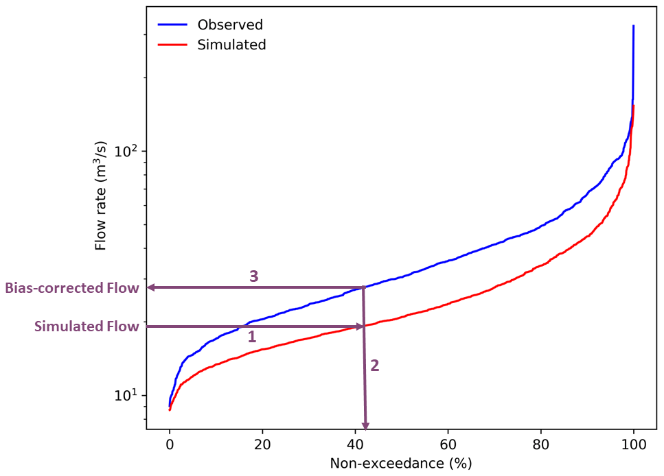
Figure 2 Conceptual diagram of quantile mapping bias correction (QM BC), showing the percentage of non-exceedance against the streamflow rate for observed (blue) and simulated (red) streamflow for GR4J an example catchment (NRFA catchment ID 12001) for the month of May. The purple arrows show the steps involved in the bias correction process: (1) for a given native simulated flow, the point on the simulated FDC (red line) is identified; (2) the non-exceedance corresponding to that simulated flow is determined; and (3) the observed flow for that same non-exceedance is determined from the observed FDC (blue line), and this value corresponds to the bias-corrected flow.

Figure 2 shows a conceptual diagram of how QM BC works. Each flow value on the simulated FDC is replaced with the flow value of the observed FDC for the corresponding non-exceedance level.

2.4 Data assimilation

DA is a group of mathematical methods which can be used to combine information from a numerical model (here a hydrological model) with available observations to generate an improved estimate of the system's state and, consequently, more accurate forecasts. DA methods can account for uncertainties associated with model structures, initial conditions, and observations and provide a probabilistic representation of the hydrological state. Here we used a particle filter (PF) technique, which uses a set of computational particles (representing possible states of the hydrological system) to estimate the most likely current state of the system.

The PF works by simulating multiple potential scenarios (particles) of the hydrological system based on the underlying model but with different sets of model parameters. The method then assigns probabilities to these scenarios based on how well they match the observed data. As new observations become available, the PF updates the particle set, giving more weight to scenarios that align with the most recent data. We updated the model parameters (production store, routing store, unit hydrograph-1 level, and unit hydrograph-2 level) in GR4J, following the implementation of Piazzi et al. (2021). We applied the particle filter approach to daily data throughout the model spin-up period (4 years) in order to improve the IHCs for the seasonal forecast. A sequential importance sampling approach was used to assign weights to individual particle states according to their likelihoods. This method is explained in more detail in Piazzi et al. (2021). We chose a PF method over a Kalman filter approach to avoid the restriction of assumed Gaussian errors and so that no mass constraints needed to be applied (see e.g. Piazzi et al., 2021). To generate the simulated observed river flows, the PF was applied once a day during the full evaluation period (1964–2015), i.e. using daily streamflow observations. Then the IHCs produced in this way at the start of each month were used to run our 612 ESP forecasts (DA-ESP).

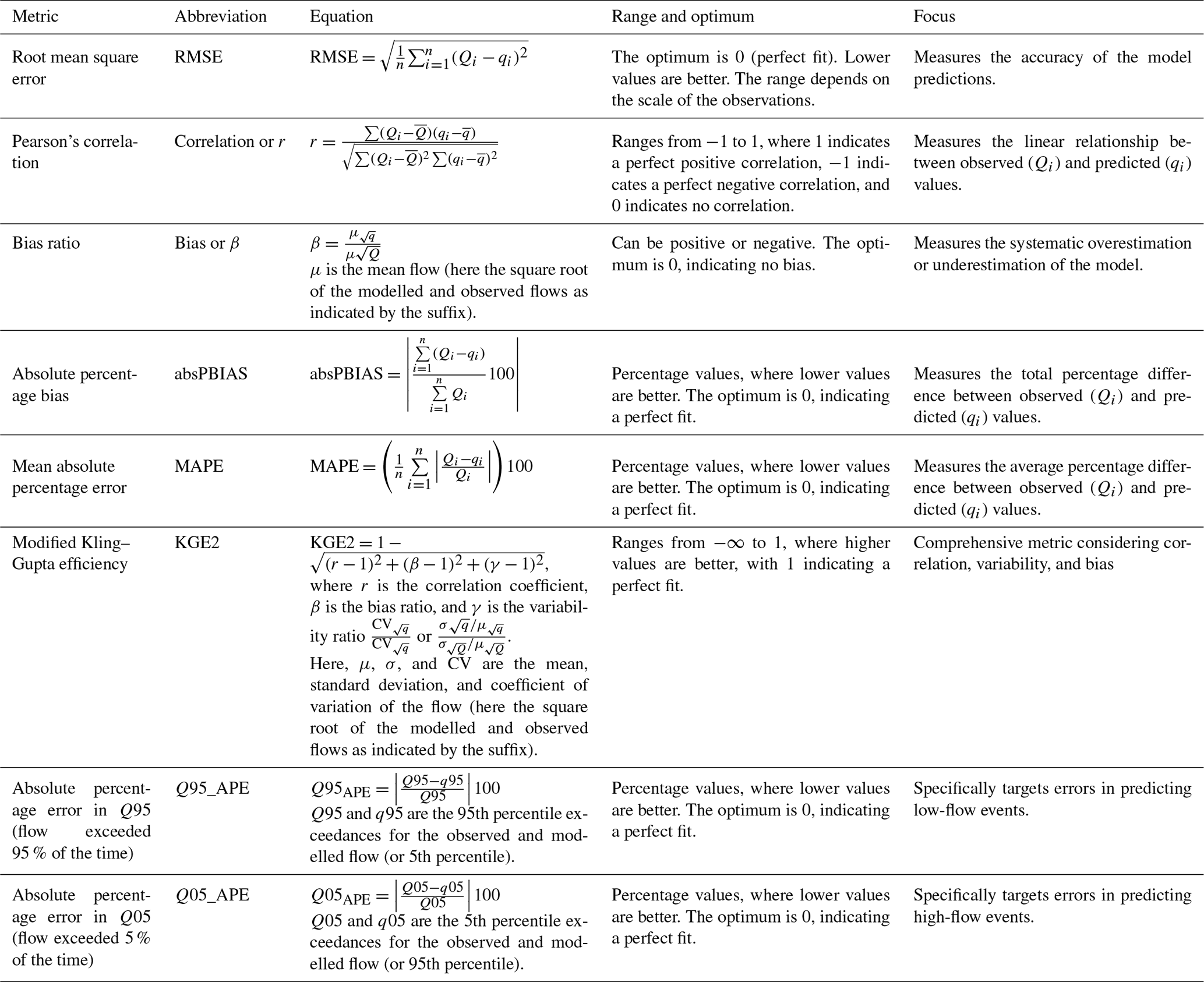
Table 2 List of performance metrics calculated with their corresponding equations. Q_i and q_i are observed and modelled flows for day i of an n daily record. $\stackrel{\mathrm{‾}}{Q}$ and $\stackrel{\mathrm{‾}}{q}$ are the mean observed and modelled flows.

2.5 Model performance evaluation

To assess the model performance and in particular compare the improvement in the simulated observed flows provided by BC and DA, we computed a range of performance metrics detailed in Table 2. These are all metrics commonly used in hydrological assessments (e.g. Hannaford et al., 2023).

2.6 Forecast skill assessment

Forecast skill refers to the relative accuracy of a set of forecasts with respect to some set of standard reference forecasts (Wilks, 2019). Even if the model performance metrics (presented in Sect. 2.5) improve with BC and DA, this is not necessarily going to translate into direct improvement in forecasting skill. This is because the enhancement achieved through DA focuses on improving IHCs, whose impact decays over lead times. Conversely, while BC is expected to enhance simulations across all lead times, its effectiveness is constrained by the inherent limitations linked to the lack of skill in the meteorological forcings, particularly in the case of ESP, which relies on climatological data.

The continuous ranked probability skill score (CRPSS; Hersbach, 2000) was used in our study to evaluate the probabilistic skill of OR-ESP, DA-ESP, and BC-ESP, using the climatology as our reference forecast like in Harrigan et al. (2018).

The CRPSS measures the relative skill of the forecast compared to a benchmark, in this case climatology. It is defined as

$$\mathrm{CRPSS}=\mathrm{1}-{\displaystyle \frac{{\mathrm{CRPS}}_{\mathrm{forecast}}}{{\mathrm{CRPS}}_{\mathrm{climatology}}}}.$$

• CRPS_forecast is the continuous ranked probability score (CRPS) of the forecast ensemble, calculated by comparing the cumulative distribution function (CDF) of the forecast to the observed data over the evaluation period.

• CRPS_climatology is the CRPS of the climatology (our benchmark), calculated by comparing the CDF of the climatology (our benchmark) to the observed data over the same period.

The CRPSS values are interpreted as follows:

• CRPSS = 1 – the forecast has perfect skill.

• CRPSS = 0 – the forecast has no skill compared to the climatology (the forecast is as good as using the climatology).

• CRPSS < 0 – the forecast is less accurate than the climatology (the forecast is misleading and has no skill).

The CRPSS penalises biased forecasts and those with low sharpness (Wilks, 2019). The Ferro et al. (2008) ensemble size correction for the CRPS was applied to account for differences between the number of members in the hindcasts (51 members, corresponding to the historic period from 1961 to 2015 with the L3OCV approach) and the benchmark (47 members, corresponding to the period of 1965–2015 with the L3OCV approach and with 4 years removed for the spin-up period), as done in the evaluation of hydrological ensemble forecasting elsewhere (e.g. Crochemore et al., 2017). Calculation of the skill scores was undertaken using the open-source easyVerification package v0.4.2 in R (MeteoSwiss, 2017).

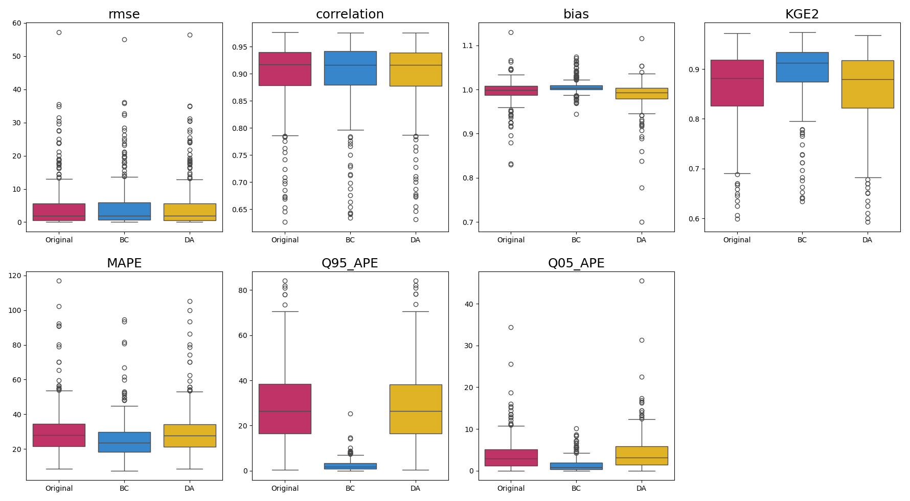
Figure 3 Model performance metrics for river flow simulations produced by the GR4J model with no additional processing (dark pink), GR4J with BC (blue), and GR4J with DA (orange) for all 316 catchments (Fig. 1b). For almost all of the performance metrics, the GR4J with BC and GR4J with DA differ significantly from GR4J model with no additional processing at the 5 % significance level, based on a Student’s t test.

To construct the time series for the CRPSS calculation, the model forecast is initialised on the first day of each month, after which the model runs freely for a lead time of up to 365 d, producing a forecast for each subsequent day at progressively longer lead times. For that month, no further initialisations are performed beyond the first day. Thus, all lead times (e.g. 1 d, 3 d, or 7 d) are calculated relative to the first day of the month. The CRPSS is then calculated based on the accumulated flow over the full forecast period rather than point values on specific days. For example, for the 7 d forecast horizon, the skill score is based on the total flow accumulated over the first 7 d of the forecast, not the streamflow value at precisely day 7. This approach better reflects the overall forecast performance for each lead time by considering the cumulative discharge over the given period.

The calculation of the CRPSS requires selection of a benchmark against which the forecasting system is evaluated. A forecasting system is considered “skilful” if its performance surpasses that of the chosen benchmark. Common benchmarks for hydrological forecast evaluation include climatology (long-term average flows), persistence forecasts (assuming the current state remains constant and commonly used for short-range forecasts), and gain-based benchmarks (using simpler models to quantify the added value of more complex models; Pappenberger et al., 2015). In this study, we selected climatology as the benchmark for evaluation, as it is a widely used reference for assessing sub-seasonal to seasonal forecasts.

Unlike Harrigan et al. (2018), who employed simulated observed river flows as the “truth” for skill evaluation, our study relies on observed flows. This choice ensures a fair comparison between OR-ESP, DA-ESP, and BC-ESP. Considering DA's objective of using observations to enhance models, using simulated observed data as the reference would have adversely affected the skill assessment of DA.

The performance metrics (Sect. 2.5) were calculated for the simulated observed flows produced by the three methods (OR, BC, and DA), and skill scores (Sect. 2.6) were calculated for all three versions of the hindcasts (OR-ESP, BC-ESP, and DA-ESP). To assess whether the differences in performance metrics and forecast skills are statistically significant, we applied a paired t test to the performance metrics and CRPSS values calculated across the 316 catchments. In all of the cases, we compared the OR simulations with the DA and BC simulations to evaluate the overall improvements introduced by the new approaches relative to the original method and to determine whether these differences are statistically significant.

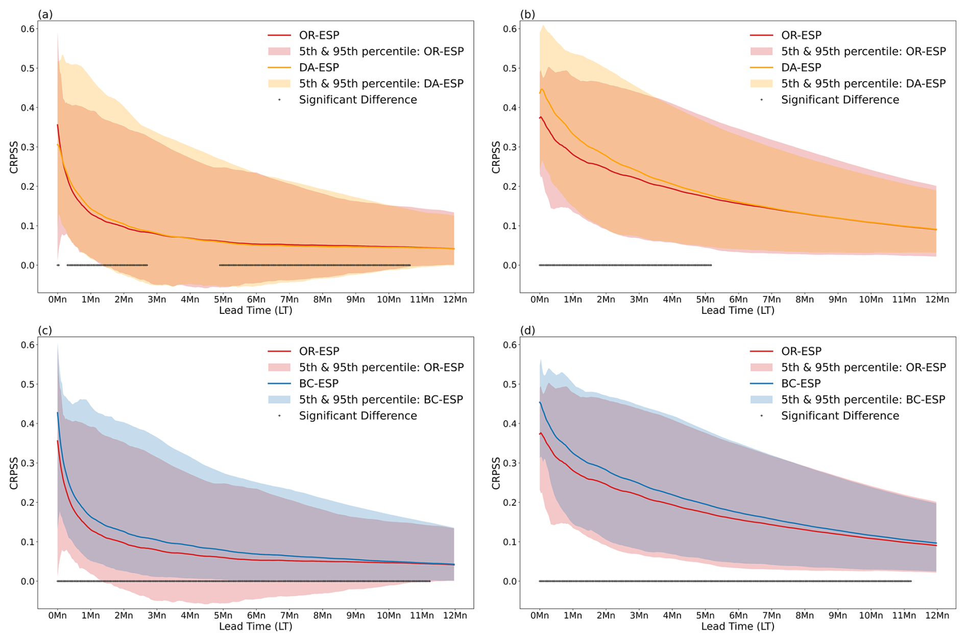
Figure 4 (a) CRPSS for all stations with < 5 % missing observations for OR-ESP (red) and DA-ESP (orange) simulations over lead times. (b) CRPSS for all stations with < 5 % missing observations and BFI > 0.6 for OR-ESP (red) and DA-ESP (orange) simulations over lead times. (c) CRPSS for all stations with < 5 % missing observations for OR-ESP (red) and BC-ESP (blue) simulations over lead times. (d) CRPSS for all stations with < 5 % missing observations and BFI > 0.6 for OR-ESP (red) and BC-ESP (blue) simulations over lead times. The solid lines show the median CRPSS, whereas the shaded areas show the catchment spread of the 5th–95th percentiles. The black plus markers indicate the lead times where BC-ESP or DA-ESP differs significantly from OR-ESP at the 5 % significance level, based on a Student's t test.

We have also calculated other skill scores, i.e. the mean absolute error skill score (MAESS) and the mean square error skill score (MSESS). However, these are deterministic skill scores and therefore less suited than the CRPSS to ensemble forecast verification. Hence, we only show CRPSS results in the following sections for brevity. The results were very similar to the ones presented here when using alternative skill scores.

3 Results

3.1 Model performance

BC and DA both improve the overall model performance in the simulated observed flows (Fig. 3), though in DA the improvement is only marginal and not for all metrics, whereas for BC the difference is more substantial and is generalised for all of the metrics considered.

The greater impact on model performance observed in BC compared to DA is unsurprising given the fundamental differences in their approaches. In BC, observations serve as the absolute truth, guiding adjustments to align simulations with the observed FDCs. As its name implies, BC is explicitly designed to rectify predictions by conforming them to observations, thus naturally yielding improvement in overall performance. Conversely, DA endeavours to enhance predictions through a mechanistic, physically informed approach during model simulation. In DA, both model-generated and observed values are weighed, aiming to refine the model's alignment with observed data while preserving the hydrological model's structural integrity. Consequently, it is expected that DA may exhibit comparatively lower performance due to the complex interplay between model fidelity and alignment with observed data.

3.2 Forecast skill improvement with data assimilation

Figure 4a shows the evolution of the skill score (CRPSS) with lead times for OR-ESP and DA-ESP for all catchments with less than 5 % missing data. We can see in this figure that, overall, there is no big improvement in skill with DA (no difference in the median skill score). However, the envelope is wider at the top end, especially for very short lead times, suggesting that DA does make a difference for some catchments.

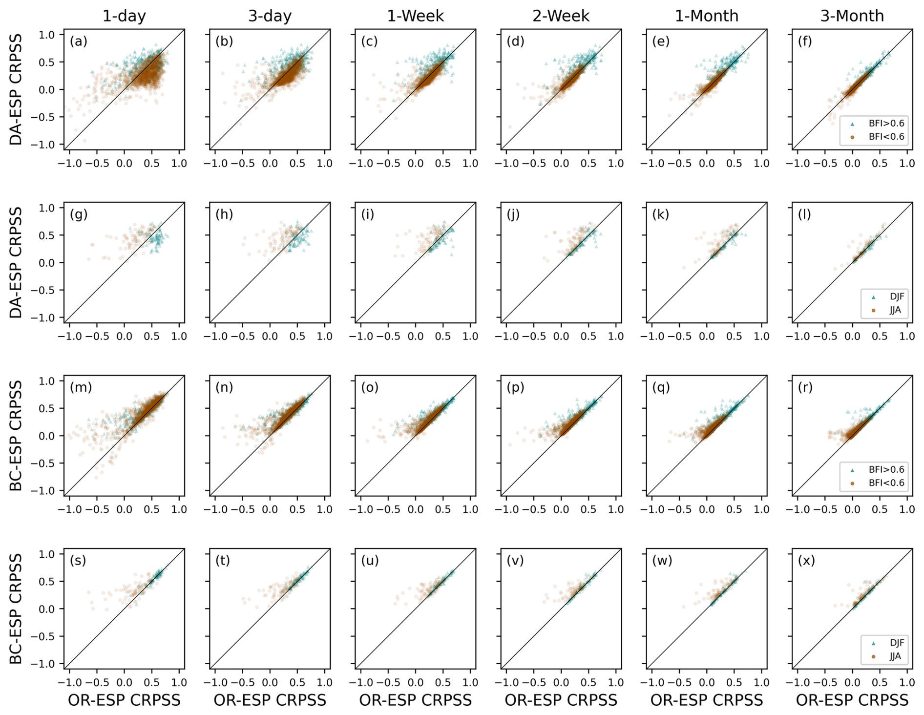
Figure 5 (a–f) Scatterplots of the CRPSS between OR-ESP and DA-ESP for all catchments with less than 5 % missing observation data, broken down according to the BFI of the station, with a low BFI < 0.6 (brown dots) and a high BFI > 0.6 (green triangles). (g–l) Scatterplots of the CRPSS between OR-ESP and DA-ESP for all stations with < 5 % missing observations and a BFI > 0.6, broken down according to season: December, January, and February start months (DJF, winter; green triangle) and June, July, and August start months (JJA, summer; brown dots). (m–r) Same as panels (a–f) but for BC-ESP instead of DA-ESP. (s–x) Same as panels (g–l) but for BC-ESP instead of DA-ESP. Forecasts are initialised on the first day of each month. The subplots within each category show increasing lead times (d).

If we look at the same comparison for catchments with BFI > 0.6 only (Fig. 4b), the improvement with DA is more notable. This improvement is observed for lead times of up to a season (∼ 3 months). After that, the effect of improved initial conditions diminishes.

Figure 5a–f show differences in skill (comparing skill for the OR-ESP on the x axis and skill for the DA-ESP on the y axis) in more detail for different types of catchments (low and high BFI values) and different lead times. The improvement in skill with DA is more apparent for higher-BFI catchments, especially for lead times of 3 to 30 d (as there are more green triangles above the 1:1 line). We also observe that catchments with a high BFI exhibit greater overall skill, which is reflected in higher CRPSS values for both OR-ESP and DA-ESP, which is in line with findings of Harrigan et al. (2018). Figure 5g–l show results for high-BFI catchments only and with a breakdown between seasons: winter (green triangles) and summer (brown dots), with forecasts initialised on the first day of each month within these seasons. We can see that the improvement brought by DA is much stronger in summer, especially at short lead times.

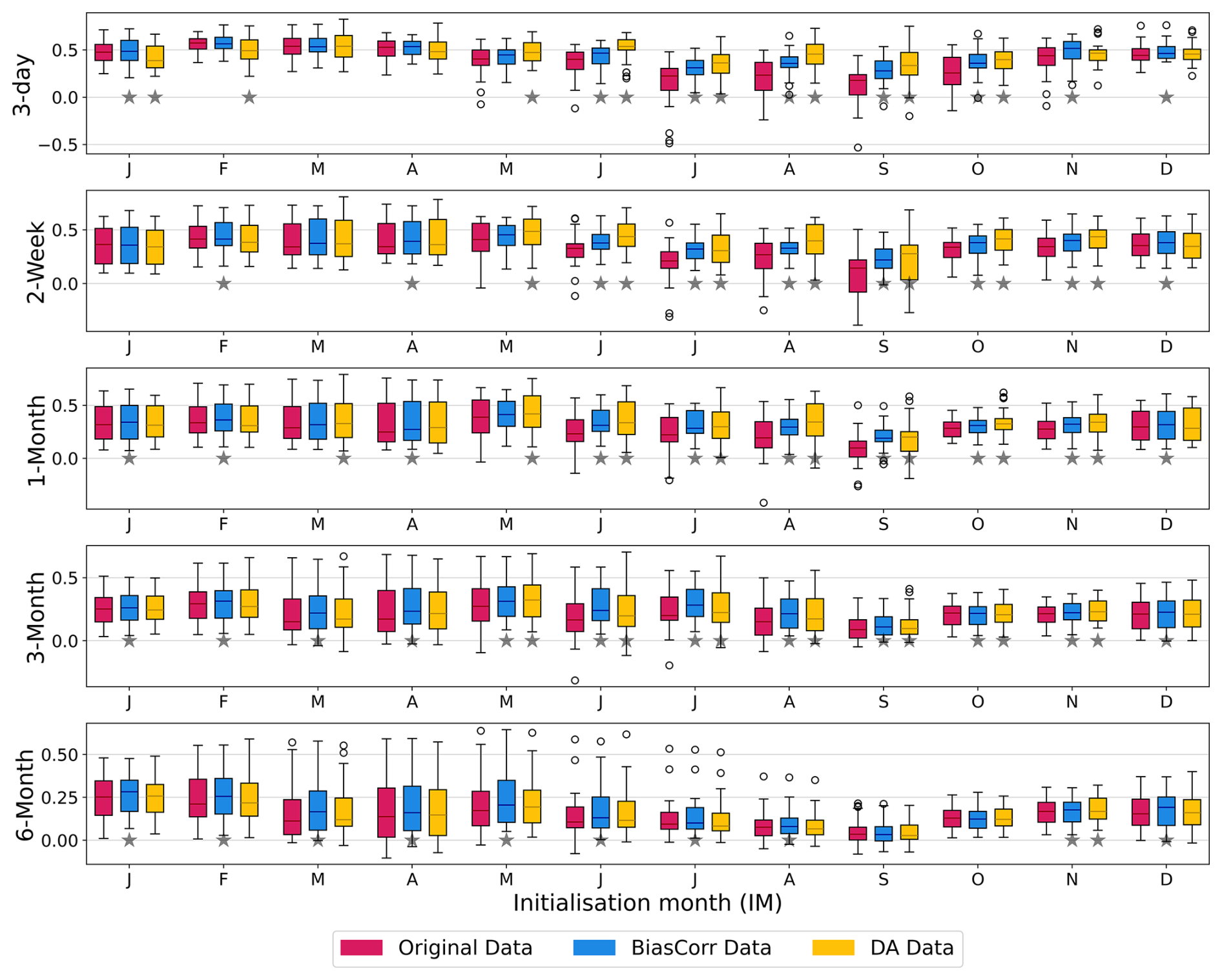
Figure 6 CRPSS values of OR-ESP, BC-ESP, and DA-ESP forecasts at different lead times and initialisation months for catchments with < 5 % of missing data and BFI > 0.6. Grey stars indicate where BC-ESP or DA-ESP differs significantly from OR-ESP at the 5 % significance level, based on a Student's t test. The “initialisation month” here refers to the month when the forecast was launched. This month marks the beginning of the forecast period, and it coincides with the start of the forecast time series data. The equivalent figure for all catchments with < 5 % of missing data can be found in Appendix Fig. A6.

3.3 Forecast skill improvement with bias correction

In the case of BC, the improvement in skill is longer-lasting and more generalised (Fig. 4c). Moreover, there is not such a clear difference in improvement between catchments with BFI > 0.6 and the rest (Fig. 4c versus Fig. 4d). Notably, BC improves the skill of even the most poorly performing catchments, as evidenced by the upward shift of the lower bound of the skill envelope (Fig. 4c), ensuring that all catchments achieve positive skill scores, in contrast to the performance of DA.

Figure 5m–x mirror Fig. 5a–l but focus on BC instead of DA, comparing the skill of OR-ESP and BC-ESP across various catchment types (Fig. 5m–r) and seasons (Fig. 5s–x). In this case, no discernible difference in skill improvement between high- and low-BFI catchments is evident with BC (Fig. 5m–r). However, we can see that the improvement in skill is greater for catchments with poor original performance. When narrowing our focus to high-BFI catchments alone (Fig. 5s–x) and investigating the seasonal effect, we observe that, similarly to DA, skill enhancements are more prominent in summer with BC as well, although to a lesser extent than with DA. This general tendency of better skill in summer is also true for all catchments in the case of BC (not shown).

The greater predictive ability of the bias-corrected forecast compared to the climatology can be attributed to the role of initial conditions in hydrological forecasting. The GR4J model is initialised using hydrological simulations driven by observed meteorological data, providing a strong foundation for the forecast. This accurate initialisation, combined with the hydrological memory of the system, enhances forecast skill, even at longer lead times. In contrast, climatological forecasts do not adjust initial conditions and lack this model-based foundation, which is why the bias-corrected model outperforms the climatology despite being driven by the historical meteorology.

3.4 Data assimilation versus bias correction

In comparing forecast skills for DA and BC at different lead times and seasons for catchments with BFI > 0.6 (Fig. 6), distinctive patterns emerge: in summer, up to a 1-month lead time, DA-ESP outperforms OR-ESP and BC-ESP, whereas BC exhibits higher improvement in skill over winter and at longer lead times. The notable suitability of DA for summer months in high-BFI catchments (i.e. with a high hydrological memory) underscores the importance of accurate IHCs during drier periods. During such periods, precipitation tends to be closer to the climatology, which is what is used to drive ESP. Getting IHCs right through DA in these situations will have a long-lasting effect.

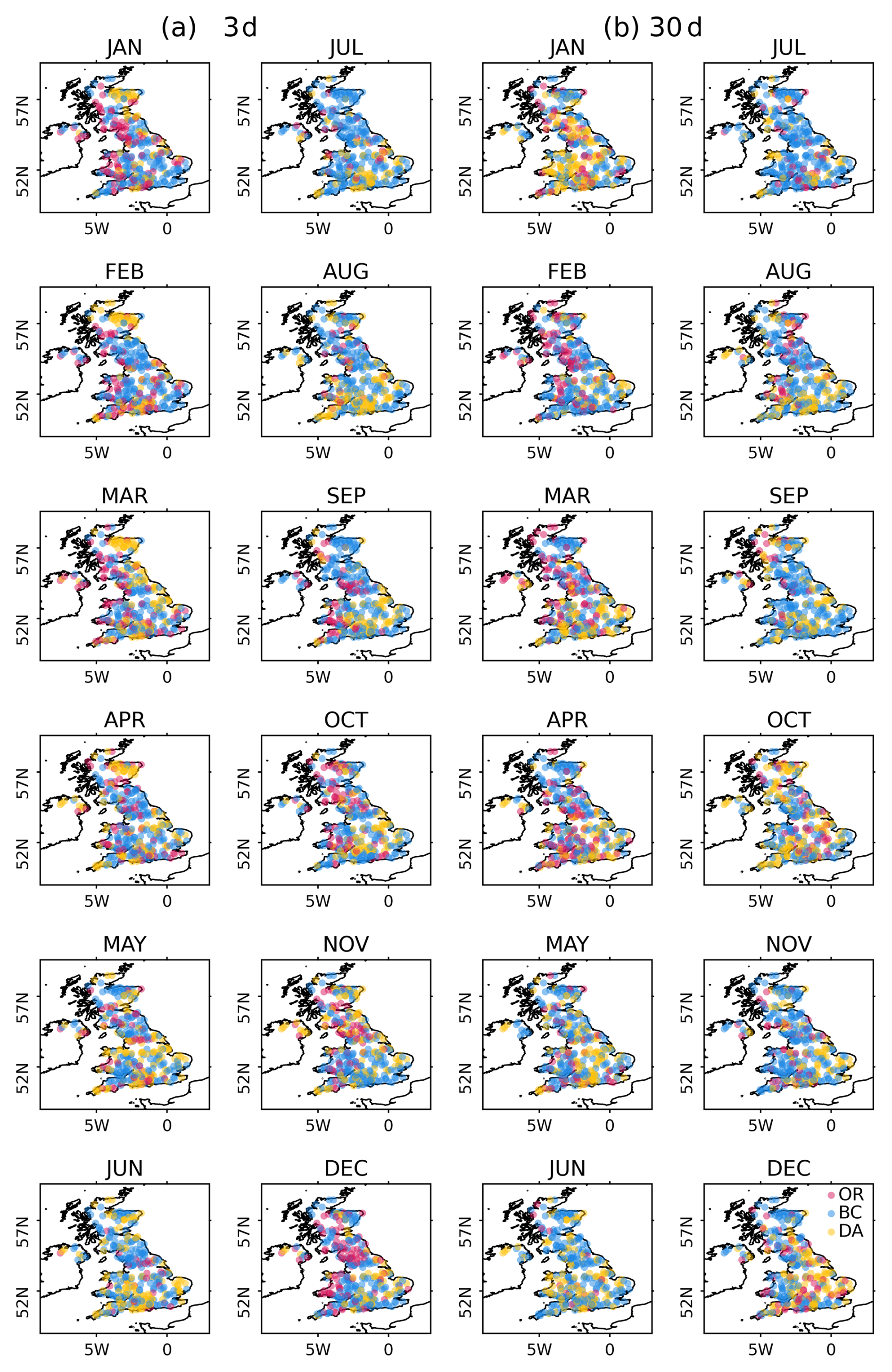
Figure 7 Each catchment showing the best-performing method (OR-ESP in red, BC-ESP in blue, and DA-ESP in yellow) based on the CRPSS for each month at lead times of (a) 3 d and (b) 30 d.

Figure 7 (which displays all 316 catchments) shows spatial differences, notably with DA showing better performance in snow-dominated catchments during winter and spring, especially for short lead times in north-eastern Scotland (Fig. 7a). Figure A7 shows the fraction of precipitation falling as snow for catchments across the UK. The version of GR4J used in this study lacks the capability to model snow accumulation and snowmelt processes, making it less reliable in catchments affected by them. DA is especially effective at adjusting the IHCs during seasons influenced by snow, such as winter accumulation and spring melting, when errors in IHCs can be large. However, for longer lead times (Fig. 7b), while no distinct patterns emerge, BC generally exhibits better performance across the majority of the catchments over most months. This observation suggests a nuanced interplay of factors influencing forecast skill, with BC showing a more consistent advantage in extended lead times across diverse catchment conditions. As mentioned previously, this can be attributed to the fundamental differences in both methodologies.

It is also interesting to note that there are cases where OR-ESP is better than both DA-ESP and BC-ESP (magenta points in Fig. 7), especially in autumn, in winter, and at the beginning of spring (October to March) in the western part of the country for short lead times (Fig. 7a) and in spring for longer lead times (Fig. 7b) with no clear spatial pattern.

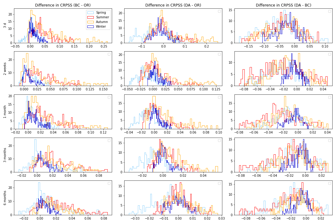
Figure 8 Histogram showing the difference in CRPSS values across 316 catchments between BC-ESP and OR-ESP (first column), DA-ESP and OR-ESP (second column), and DA-ESP and BC-ESP (third column) for various lead times (rows) and seasons (colours). Positive values indicate that the CRPSS value of the first ESP version in each pair is greater than the second (indicating higher skill).

Figure 8 presents a series of histograms illustrating the differences in the CRPSS across various versions of ESP for all 316 catchments, showcasing the extent and variations in improvement offered by BC and DA across different seasons and lead times. Examining the first two columns of subplots (the first column comparing BC-ESP and OR-ESP and the second column comparing DA-ESP and OR-ESP), we observe some similarities: (i) the range of differences between the corrected (BC or DA) and original (OR) ESPs is narrower in winter (dark blue) and widest in autumn (orange); (ii) spring (light blue) exhibits the most cases where OR-ESP outperforms both BC-ESP and DA-ESP (indicated by the negative values in the histograms); (iii) for both methods (BC and DA), the greater gains in skill are achieved in summer and autumn; and (iv) for lead times longer than 3 months, the differences between the different ESP versions are minimal, with absolute values < 0.08 for BC-ESP versus OR-ESP and < 0.03 for DA-ESP versus OR-ESP, suggesting negligible improvement beyond this point. Therefore, the gain achieved beyond 3 months using either technique is marginal.

Focusing now on the differences between DA and BC, we can see that, in general, BC presents fewer negative instances compared to DA, indicating that BC-ESP outperforms OR-ESP more frequently than DA-ESP. However, the magnitudes of improvement are typically comparable for lead times of less than 3 months for both methods. Directly comparing the CRPSS of DA-ESP and BC-ESP (third column of subplots in Fig. 8), we observe a skew towards negative values, indicating more instances where BC outperforms DA. Nonetheless, beyond a 2-week lead time, the absolute differences are negligible (< 0.08), suggesting that both methods yield similar outcomes.

4 Discussion

4.1 Bias correction versus data assimilation

Despite their shared goal of enhancing forecast accuracy, it is important to recognise the fundamental and conceptual differences between the DA and BC methodologies. As already mentioned, BC operates as a post-processing technique, rectifying model errors after simulations, while DA intervenes during model initialisations, adjusting model internal states to nudge simulations towards observed data. DA, as used here, primarily focuses on refining initial conditions and hence yields more significant impacts on catchments with a high BFI due to the extended hydrological memory. DA also proves superior at short lead times for snow-dominated catchments, where the IHCs can be widely wrong due to the lack of explicit representation of snow accumulation and snowmelt processes in the hydrological modelling used in this study. Although the GR4J model does not include a dedicated snow module, snowmelt and accumulation processes are likely captured indirectly through other model dynamics. Data assimilation updates the model state, improving the simulation of these processes even without explicit representation. As Cooper et al. (2021) note, updated parameters in models like JULES can implicitly correct for processes not directly included in the model, such as groundwater dynamics. Similarly, GR4J may implicitly account for snow-related processes through data assimilation, provided there are sufficient observational signals. One future improvement would be to explicitly include snow processes, e.g. by using GR4J-CemaNeige. This would enable a comparison of updated parameters and provide insight into how snow processes influence parameter values.

In contrast to these enhancements at short lead times yielded by DA, BC extends its improvement beyond the initial conditions, improving the quality of the simulations throughout the entire time series. However, it is noteworthy that the DA and BC methods also fundamentally differ in their handling of uncertainties. DA methodologies based on Bayesian statistics, such as PF, account for uncertainties associated with model structures, initial conditions, and observations, providing a probabilistic representation of the hydrological state. This probabilistic nature enables a more thorough understanding of the forecast, acknowledging the inherent uncertainty in predicting natural systems. Additionally, DA offers the advantage of maintaining the structural integrity of the hydrological model. In other words, a model with DA-updated initial conditions preserves the relationships between the model state and the target variable, while BC can alter them. Moreover, BC, while effectively aligning model outputs with observations, may inadvertently mask or underestimate the uncertainties in the hydrological model and observational data. The deterministic nature of BC can oversimplify the complex interplay of factors influencing streamflow predictions and uncertainties in observations, potentially leading to an overconfident representation of forecast accuracy.

While the handling of uncertainties distinguishes DA from BC, it is imperative to consider the associated computational demands and implementation complexities, especially if they are to be implemented operationally. This introduces a pragmatic dimension into the comparison, as the choice between DA and BC necessitates a nuanced evaluation of their distinct features and trade-offs. DA's computational demands and implementation complexity starkly contrast with the simplicity and ease of implementation offered by BC, positioning the latter as an accessible “easy win” for swiftly enhancing forecasting products. Our results reveal an absence of universal superiority of one method over another, underscoring their dependency on catchment characteristics, seasonal dynamics, and lead times. Interestingly, there are cases where the uncorrected OR-ESP outperforms both DA-ESP and BC-ESP, even at shorter lead times (Fig. 7). Therefore, based on our findings, for the UK, we recommend selectively applying DA for short lead times in summer and catchments with a high BFI and for catchments affected by snow accumulation and snowmelt in winter and spring at short lead times, which is where the greatest benefit of DA was observed (Fig. 6). In the rest of the cases, BC is the recommended method. Alternatively, the exclusive use of BC is advocated as a pragmatic, efficient solution, particularly where computational costs pose a limitation. Figure 8 shows that, even in the rare cases where OR-ESP outperforms BC-ESP, it does so with only marginal differences in the CRPSS. This ensures that the hydrological post-processing is not “doing any harm” to the inherent skill of the raw model outputs (Hopson et al., 2020).

It should be noted that applying both BC and DA simultaneously to harness their combined effect is not straightforward. This complexity arises from the fact that the FDC used for quantile mapping relies on observed flow data without incorporating data assimilation. Thus, introducing data assimilation would disrupt the established relationships that underpin the quantile mapping method. However, the two methods are not mutually exclusive, and combining them could be evaluated in future work. This would require a different experimental setting to ensure the applicability of QM BC in simulations that have undergone data assimilation.

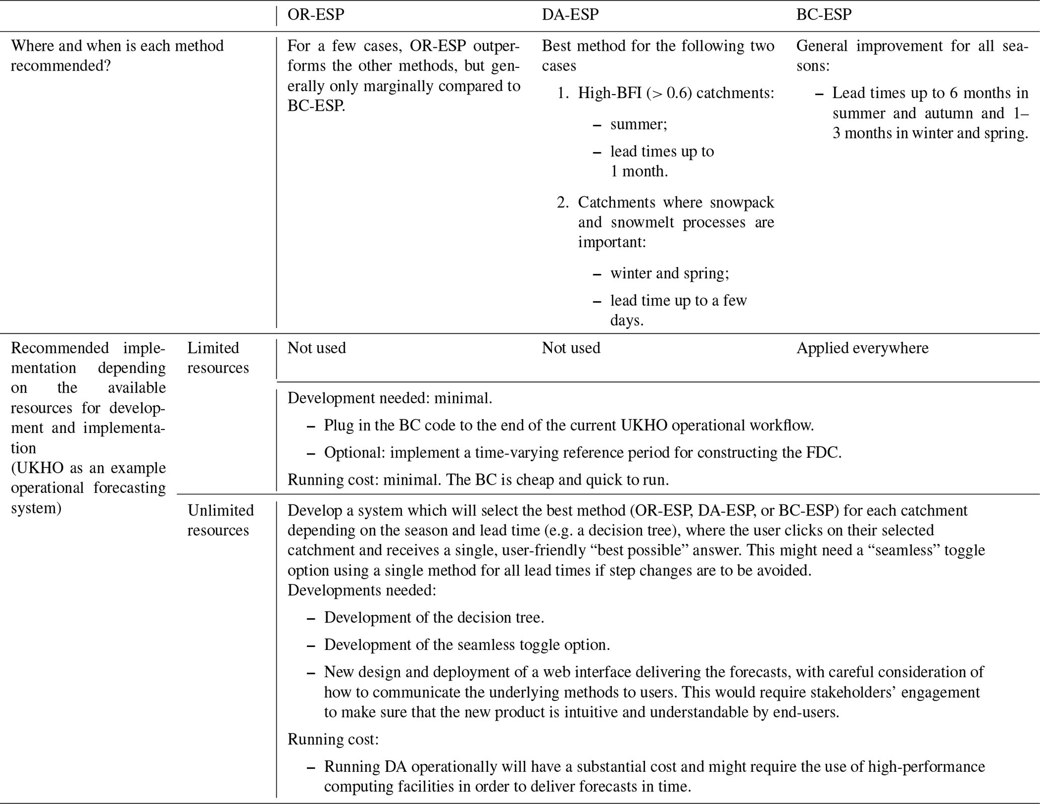
Table 3 “Best” method and recommended implementation based on the available resources.

4.2 Model improvements versus practical needs: a fine balance

Many argue that science should focus on enhancing hydrological models rather than correcting their errors by post-processing (BC) or “nudging” their parameters through data assimilation (Refsgaard et al., 2023). While such advancement is undoubtedly crucial for deepening our comprehension of the physical world (Beven, 2019), this type of research is much slower to conduct, and incremental improvements take time to translate into impact for users. We could even argue that no model will ever perfectly simulate the physical world. For example, human influence is notoriously difficult to account for in hydrology. This slowly evolving advancement of the models is asynchronous with the urgent need of end-users to have reliable outputs that they can trust to base their decision-making on (e.g. Cassagnole et al., 2021; Li et al., 2019; Pappenberger, 2024). It is worth noting the practical implications of improving hydrological forecasts (Lopez and Haines, 2017; Neumann et al., 2018), particularly in the context of operational use by decision-makers, whereby the difference between correcting or not correcting a forecast – regardless of the method being used – can determine whether they are deemed useful and consequently used by stakeholders or not (Hopson et al., 2020). The Hydrological Outlook UK, which is the subject of this case study, serves as a pertinent example of the real-world application of forecast products.

Moreover, incremental refinements in hydrological models often result in only marginal enhancements to forecast skill, as illustrated by plots in the Appendix comparing the GR4J and GR6J models (Fig. A1). Notably, the difference in forecasting skill between these models is minimal, highlighting the challenge of achieving substantial gains through model enhancements alone. In contrast, our assessment demonstrates that methods like BC yield more significant and immediate improvements in forecast accuracy. Therefore, in parallel with the ongoing efforts to enhance the cores of hydrological models, exploring methods – such as BC and DA – to refine existing forecasting products becomes justified. This paper consistently assesses and compares two of these methods, offering evidence of the benefits they deliver and providing a pragmatic solution to refine existing forecasting products, meeting the pressing demand from end-users for reliable outputs that inform their decision-making.

4.3 Post-processing methods in hydrological forecasting

In the broader context of hydrological research, our study's exploration of BC and DA methods contributes to the ongoing dialogue surrounding hydrological forecast post-processing techniques. While machine learning (ML) methods like convolutional neural networks (CNNs) and support vector regression (SVR) have shown promise in enhancing forecast accuracy (Liu et al., 2022), their computational demands present challenges. Notably, our study employs QM for BC, a computationally efficient method, distinguishing it from more resource-intensive ML approaches.

In similar work, Matthews et al. (2022) adopt a post-processing method derived from the Multi-Temporal Model Conditional Processor (MT-MCP; Coccia and Todini, 2011). They find a pronounced impact in catchments with a long hydrological memory. A key difference with our work lies in their use of numerical weather prediction (NWP) as the driving data, contrasting with our reliance on climatological weather input for the ESP method. This distinction implies that their hydrological forecasts, particularly in dynamic or “flashy” catchments, are sensitive to the skill of NWP input, potentially diminishing the relative effectiveness of post-processing compared to our experimental setting in those catchments. In that sense, ESP serves as an ideal test case to isolate the value of the DA and BC methods given the absence of skill from the meteorological forecast to “take over” from the IHCs.

Additionally, we acknowledge the challenge of non-stationarity in QM, a concern highlighted by Ceola et al. (2014). To address this, in an operational setting, incorporating real-time updates by dynamically adding the newest observed data would be done, allowing the FDC to adapt monthly. A potential refinement could be explored by changing reference periods, such as the most recent 30-year period, offering a dynamic approach to account for non-stationarity, albeit with the associated risk of overlooking rarer extreme events.

To the best of our knowledge, no prior study has undertaken a direct comparison between BC and DA, a gap that might be attributed, in part, to the inherent disparities between these two methodologies, as mentioned already. Nevertheless, from a users' standpoint, such a comparative analysis holds significant value. It facilitates the selection of the optimal forecasting product tailored to distinct situations, offering valuable insights for decision-makers seeking to enhance the reliability of their hydrological forecasts.

4.4 Limitations and future work

The present study naturally has some limitations given the practicalities of applying multiple approaches across many catchments, lead times, and seasons. Firstly, the gap-filling approach employed to address missing data in the observed river flow time series is quite rudimentary, relying on a simple linear interpolation method. While this method is commonly used for gap-filling (Niedzielski and Halicki, 2023), it comes with inherent limitations, such as its sensitivity to outliers and oversimplification of the underlying hydrological processes, especially when gap-filling longer time periods. Note that both techniques (BC and DA) can be applied even if the observed data have some missing data (DA is not applied where no data are available, and BC uses whatever data are available to construct the FDC). Full time series were only needed to calculate the CRPSS used to carry out the comparative analysis. While more sophisticated techniques for handling missing data, such as data-driven methods or advanced statistical approaches, could have been considered to enhance the accuracy of the reconstructed time series (e.g. Dembélé et al., 2019; Luna et al., 2020), such methods would have significantly increased the complexity of the analysis. To mitigate this limitation, the study has focused much of its analysis on a subset of the dataset, where less than 5 % of the data were missing (Fig. 1b), minimising in that way the effect of the gap-filling (Arriagada et al., 2021). Consequently, using an alternative gap-filling method would likely have yielded comparable conclusions.

Secondly, the DA methodology implemented in this study, the PF technique, is used in a deterministic manner (where we have used the PF ensemble mean to avoid having an ensemble of ensembles) to ensure comparability with BC results. However, the PF method inherently provides valuable information on uncertainty associated with the hydrological state (e.g. Moradkhani et al., 2012). In the current study, this information on uncertainty is not fully exploited, as the analysis primarily focuses on the comparison with BC. Future investigations could explore more sophisticated approaches within DA that capitalise on the uncertainty estimates provided by the PF technique.

Building on our analysis of the comparative strengths of DA and BC, our study identified the specific scenarios where each method improves the forecasts the most. Depending on the resources available for implementation, we summarise our recommendations based on our findings in Table 3. This lays the groundwork for a prospective user-friendly hydrological forecasting system in the future that could be implemented in the operational HOUK setting. Recognising that end-users and non-specialists often prioritise a simplified and trustworthy message (Hannaford et al., 2019), we envision the implementation of a flexible, combinatory (e.g. decision-tree-based) forecasting system that would dynamically choose the most effective method based on specific factors such as catchment characteristics, time of year, and lead time. For end-users seeking “the best answer” without delving into the intricacies of the methodology, this streamlined approach aims to provide the most reliable forecast available in a clear and simple manner. While this concept would require rigorous testing and development first, it highlights a potential avenue for future research in tailoring hydrological forecasts to meet the practical needs and expectations of end-users. The cheaper, more immediate solution would be to blanket-apply BC to improve all catchments indiscriminately.

Furthermore, future studies could explore alternative post-processing methods (Li et al., 2017), such as copula-based approaches and machine learning techniques (Liu et al., 2022), or statistical and empirical post-processing methods, such as using the Hydrological Uncertainty Processor (HUP; Krzysztofowicz, 1999) and its variants such as the Model Conditional Processor (MCP, Todini, 2008). All of these options, while potentially offering improved forecast accuracy, come with varying computational expenses. Investigations into diverse post-processing methodologies can enhance our understanding of their applicability and effectiveness in different hydrological contexts, providing valuable options for refining forecasting products in the future.

5 Conclusion

In this study, we have explored the effectiveness of quantile mapping (QM), bias correction (BC), particle filter (PF), and data assimilation (DA) techniques in enhancing hydrological model performance and forecast skill, specifically focusing on improving hydrological forecasts using the ensemble streamflow prediction (ESP) method with the GR4J model for the Hydrological Outlook UK operational service. Our findings reveal that both BC and DA contribute to improvements, yet their impacts vary across different metrics and catchment characteristics.

BC, operating as a post-processing method, demonstrates substantial and generalised improvements across various performance metrics. It rectifies model errors after simulations, extending its positive influence beyond initial conditions throughout the entire time series. However, while QM BC effectively aligns statistical properties, it may oversimplify the complexity of hydrological systems by neglecting to capture the physical processes and interactions, consequently leading to an underestimation of uncertainties.

On the other hand, DA, which adjusts model internal states during initialisations to align simulations with observed data, exhibits more subtle and marginal improvements. The positive effects of DA are particularly notable in catchments with a high baseflow index (BFI) and up to the seasonal scale, and DA often yields more improvement than BC at short lead times (up to 1 month) in summer. DA also outperforms BC for catchments where snow processes are important, mainly in north-eastern Scotland in winter (snow accumulation) and spring (snowmelt) at short lead times. The probabilistic nature of DA, considering uncertainties associated with model structures, initial conditions, and observations, provides a comprehensive representation of the hydrological state.

The choice between BC and DA involves trade-offs, considering their conceptual differences, computational demands, and handling of uncertainties. While DA offers a more sophisticated approach, BC presents a pragmatic and computationally efficient solution, especially when computational costs pose a limitation. The absence of universal superiority of one method over another emphasises the importance of selectively applying these techniques based on specific scenarios, user requirements, and operational constraints. Future work could explore the combined use of both techniques, though it would need to first address the challenge of constructing the flow duration curve used in the QM method for flow simulations modified by data assimilation.

In the broader context of hydrological research, our study contributes valuable insights to the body of literature on forecast enhancement techniques. Our findings can pave the way for a more objective, on-the-fly selective forecasting system tailored to catchment characteristics, time of year, and lead time, which would be a step towards user-friendly and practical hydrological forecasting systems.

In conclusion, this research provides a novel intercomparison of QM BC and PF DA, offering an assessment of their strengths and limitations when applied to UK streamflow forecasting. By recognising the diverse contexts where each method excels, hydrologists and decision-makers can make informed choices to refine forecasting products, aligning with the ever-growing demand for reliable and actionable hydrological information.

Appendix A: Additional figures

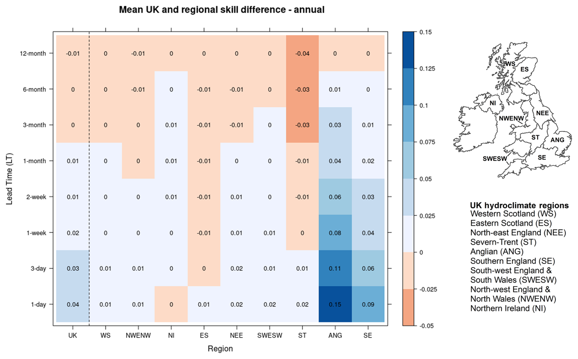
Figure A1 Change in forecasting skill (CRPSS) at different lead times when transitioning from GR4J to GR6J to produce ESP forecasts in the different UK hydroclimate regions. Blue signifies improved forecast skill with GR6J compared to GR4J, while orange represents the reverse.

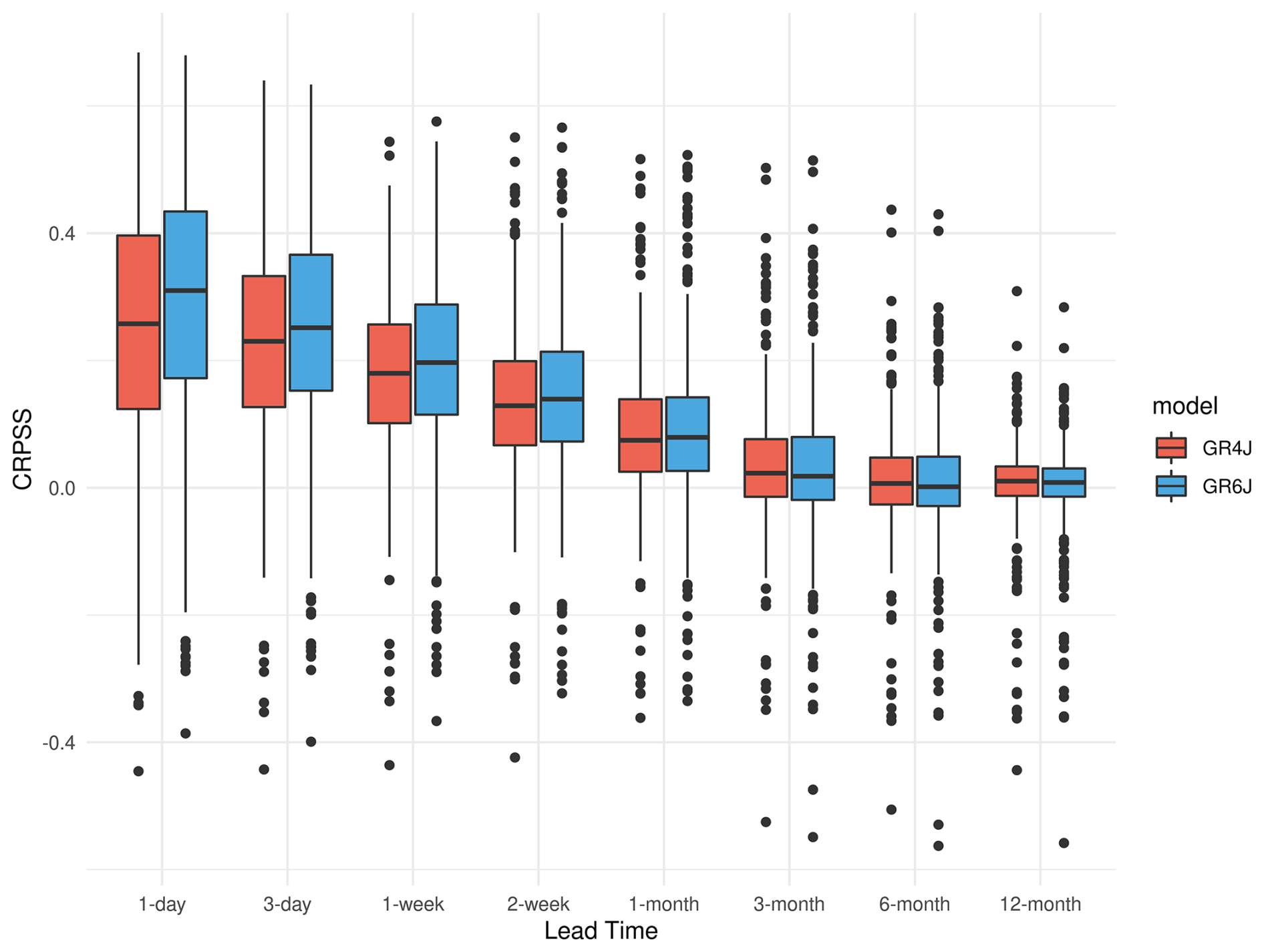
Figure A2 Boxplots showing the range of the CRPSS for all catchments used in the UKHO at different lead times in ESP forecasts generated using GR4J (in red) and GR6J (in blue).

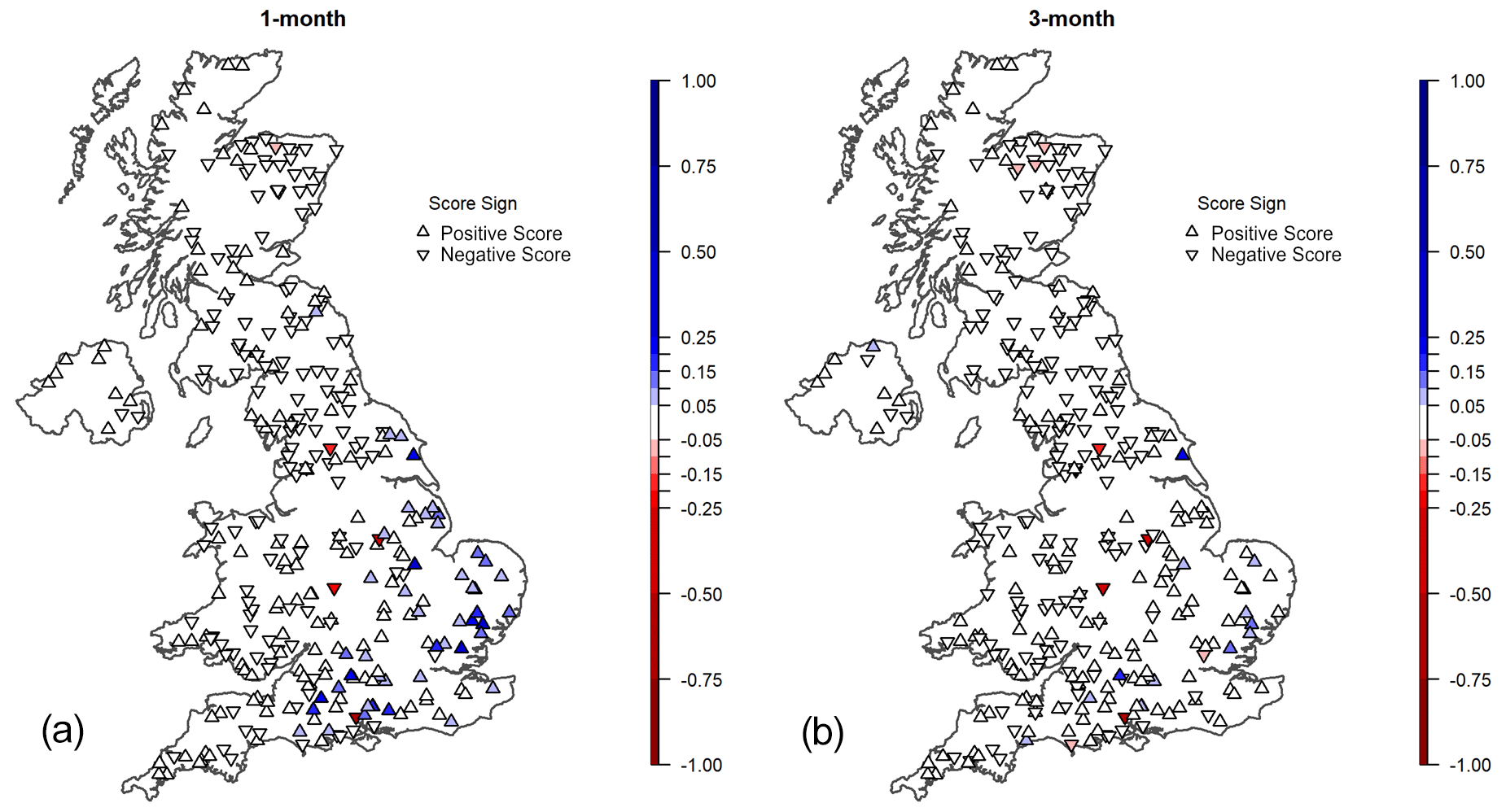
Figure A3 Map of the difference in skill (CRPSS) between ESP forecasts generated using GR6J and GR4J at (a) a 1-month lead time and (b) a 3-month lead time. Blue shades signify improved forecast skill with GR6J compared to GR4J, red shades represent the reverse, and white shades signify negligible differences (source: https://hydoutuk.net/about/methods/river-flows, last access: 18 March 2025).

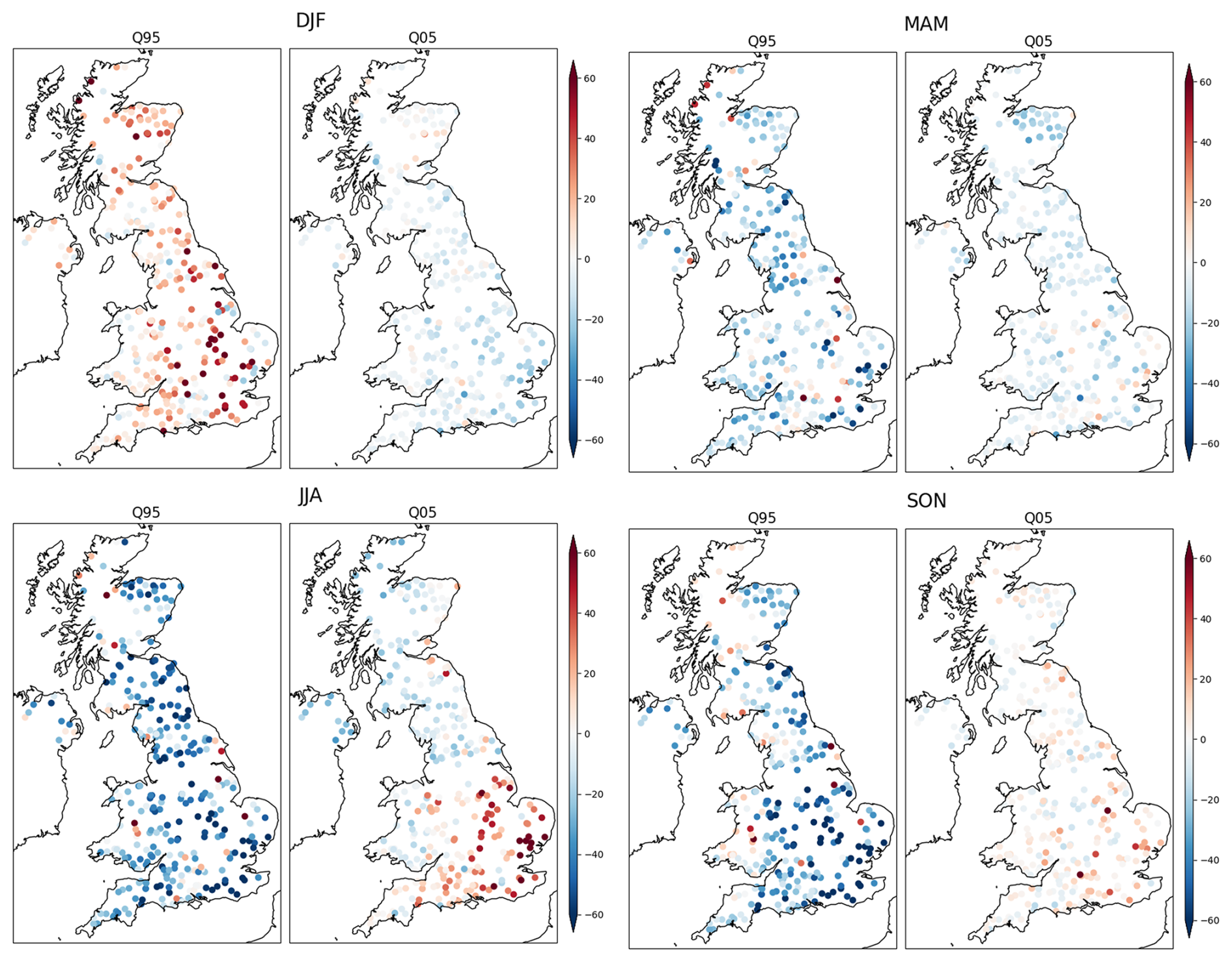
Figure A4 Percent bias for each season for low flows (Q95) and high flows (Q05) in streamflow simulated by GR4J. The percent bias is calculated as $(q-Q)/Q\times \mathrm{100}$ for the low flows (Q95) and high flows (Q05), where q is the simulated flow and Q is the observed flow. The percent bias can be negative when the simulated flow is lower than the observed flow.

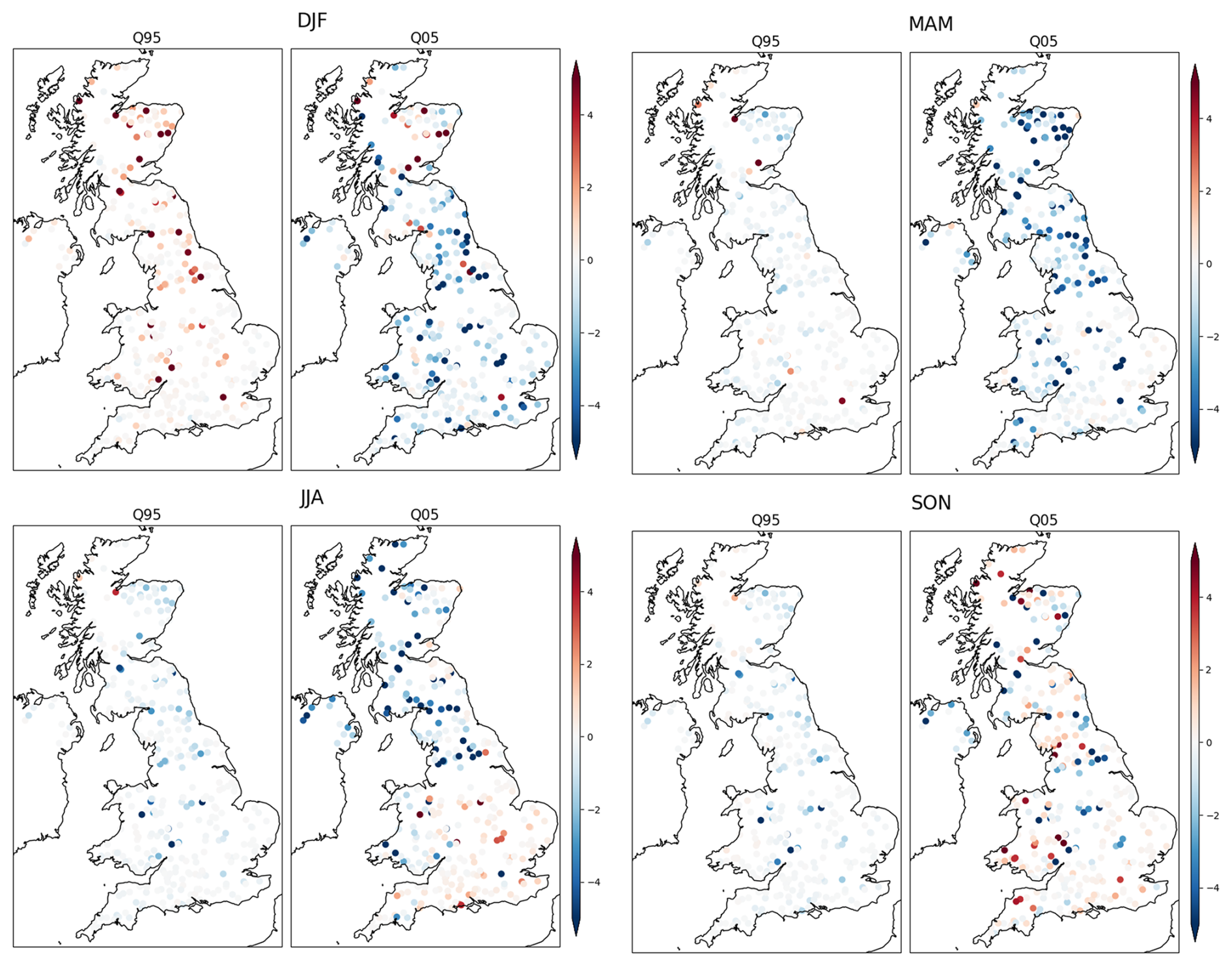
Figure A5 Bias (m³ s⁻¹) for each season for low flows (Q95) and high flows (Q05) in streamflow simulated by GR4J. The bias shown here is the raw bias, defined as (q−Q), for the low flows (Q95) and high flows (Q05), where q is the simulated flow and Q is the observed flow. The bias can be negative when the simulated flow is lower than the observed flow.

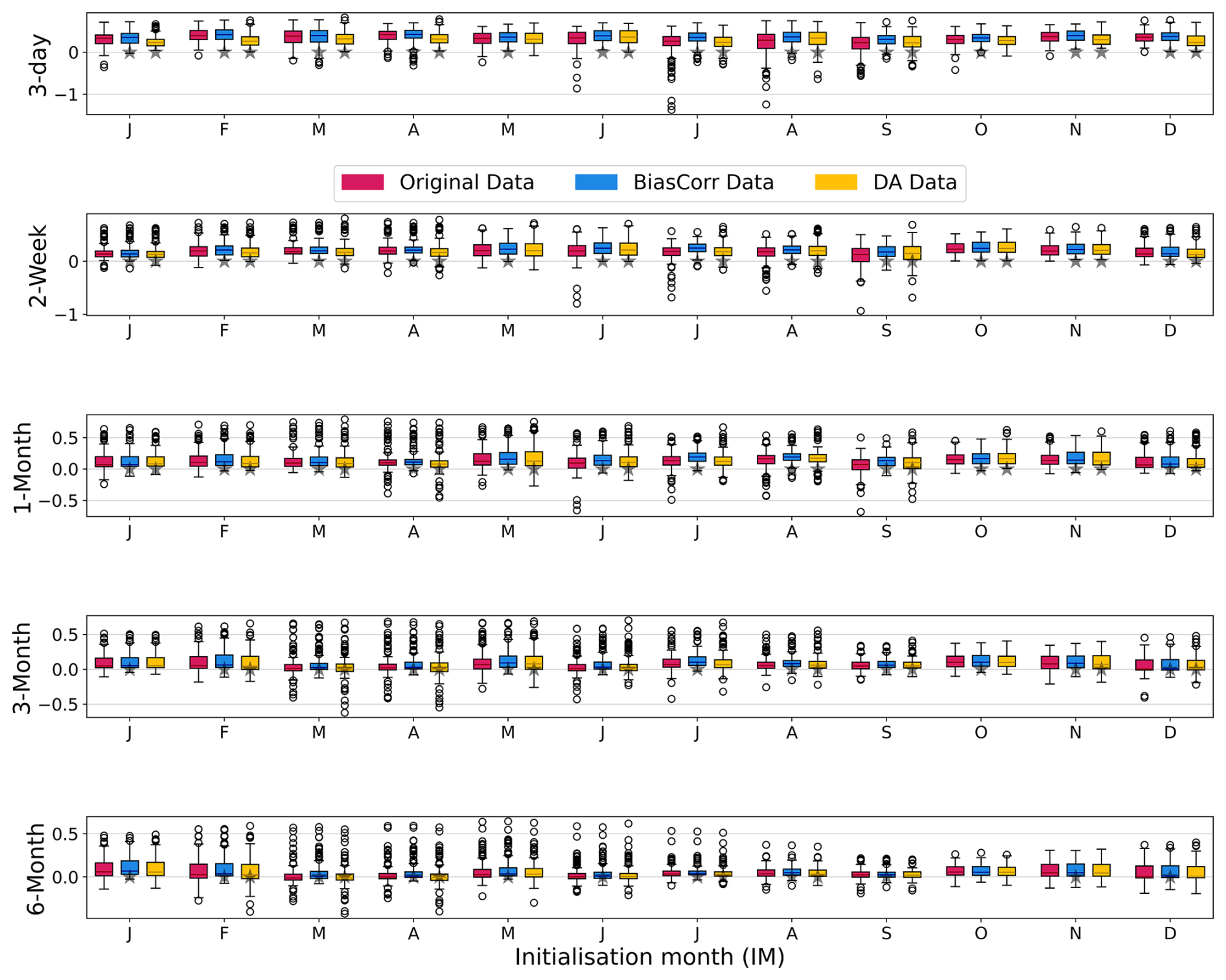
Figure A6 The CRPSS of OR-ESP, BC-ESP, and DA-ESP forecasts at different lead times and initialisation months for catchments with < 5 % of missing data. The grey stars indicate where BC-ESP or DA-ESP differ significantly from OR-ESP at the 5 % significance level, based on a Student's t test.

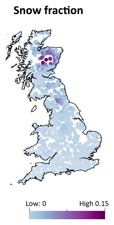
Figure A7 Fraction of precipitation falling as snow for catchments across the UK, where a value of 0.15 indicates that 15 % of the catchment precipitation falls on days when the temperature is below zero (source: Lane et al., 2019).