Economic valuation of subsurface water contributions to watershed ecosystem services using a fully integrated groundwater–surface-water model

Water is essential for all ecosystem services, yet a comprehensive assessment and economic valuation of total (overall) water contributions to ecosystem services' production using a fully integrated groundwater–surface-water model has never been attempted. Quantification of the many ecosystem services impacted by water demands an analytical approach that implicitly characterizes both subsurface and surface water resources. However, incorporating subsurface water into ecosystem services' evaluation is a recognized scientific challenge. In this study, a fully integrated groundwater–surface-water model – HydroGeoSphere (HGS) – is used to capture changes in subsurface water, surface water, and transpiration (green water use), and along with an economic valuation approach, it forms the basis of an ecosystem services' assessment for an 18-year period (2000–2017) in the 3830 km² South Nation watershed (SNW), a mixed-use but predominantly agricultural watershed in eastern Ontario, Canada. Using green water volumes generated by HGS and ecosystem services' values as inputs, the marginal productivity of water is calculated to be CAD 0.26 m⁻³ (in 2022 Canadian dollars). Results show maximum green water values during the driest years, with the extreme drought of 2012 being the highest at CAD 424.7 million. In contrast, the green water value in wetter years was as low as CAD 245.9 million, while the 18-year average was CAD 338.83 million. Because subsurface water is the sole contributor to the green water supply, it plays a critical role in sustaining ecosystem services during drought conditions. This study provides new insight into the economic contributions of subsurface water and its role in sustaining ecosystem services during droughts, and it puts forth an improved methodology for watershed-based management and valuation of ecosystem services.

1 Introduction

The role of subsurface water (including groundwater and soil moisture) in socio-economic development is widely acknowledged (Foster and Chilton, 2003); however, its ecological contributions are undervalued (Yang and Liu, 2020), despite being fundamental to the control of terrestrial ecological processes (Qiu et al., 2019). Subsurface water supports numerous ecosystem services that include provisioning, regulating, supporting, and cultural services (Griebler and Avramov, 2015). While infiltration is a driver for subsurface water recharge, subsurface water discharge and vegetation uptake are, in turn, key fluxes for supporting terrestrial ecosystems (wetlands, forests, crops, etc.) (Griebler and Avramov, 2015). Subsurface water can provide a buffer against weather stressors on vegetation and aquatic ecosystems and helps to maintain key processes that underpin ecosystem services (Qiu et al., 2019). To date, most ecosystem services' research has focused on aboveground factors and processes (e.g., land use change), and very little focus has been given to subsurface water and its influence on terrestrial ecosystem services (Richardson and Kumar, 2017; Qiu et al., 2019). While some previous research (e.g., Booth et al., 2016; Li et al., 2014) has attempted to link subsurface water with land cover, it typically reflects field-scale static environmental conditions (Qiu et al., 2019). Given the challenges with mapping subsurface water resources, the contribution of subsurface water towards terrestrial ecosystem services is not typically quantified, and the economic value of subsurface water contribution to terrestrial ecosystem services is therefore not assessed.

While hydrologic ecosystem services' studies are common in the literature (Ochoa and Urbina-Cardona, 2017), groundwater-focused ecosystem services' assessments are rare. However, groundwater can be an important regulator of watershed hydrologic behaviour and ecosystem health, especially in regions with a shallow water table, such as the Laurentian Great Lakes region (Neff et al., 2005; Kornelsen and Coulibaly, 2014). In such areas, groundwater acts as a source of soil water (Chen and Hu, 2004). The importance of groundwater has been noted by Griebler and Avramov (2015) in their review of groundwater ecosystem services, where they highlight the direct role it plays in supplying different types of ecosystem services (Millenium Ecosystem Assessment (MEA), 2005); and they stress the need for a better quantitative understanding of groundwater processes in order to protect and manage groundwater and its ecosystem services. Furthermore, Mammola et al. (2019) emphasize that subterranean ecosystems are largely being overlooked in conservation policies. Based on a preliminary assessment of all the regions around the world where groundwater plays a critical role in ecosystem services, as well as considering that approximately 43 % of consumptive irrigation is sourced from groundwater (Siebert et al., 2010), the lack of focus on subsurface water ecosystem services is not due to lack of need, rather the lack of use of suitable tools to conduct the required analysis.

Hydrological models can efficiently and accurately quantify water storages and fluxes over large spatial scales. With groundwater ecosystem services' increasing role in policymaking (Honeck et al., 2021) and sustainable groundwater resources management, new tools are required for their mapping. At present, common modelling tools available for ecosystem services' mapping include relatively simple matrix models (i.e., Decsi et al., 2022) and more complex models such as ARtificial Intelligence for Environment & Sustainability (ARIES) (Villa et al., 2021), Co$ting Nature (Mulligan, 2015), Envision (Bolte, 2022), and Integrated Valuation of Ecosystem Services and Tradeoffs (InVEST) (Natural Capital Project, 2022), with InVEST being by far the most prominent in the scientific literature (Ochoa and Urbina-Cardona, 2017). However, models specific to ecosystem services, such as the InVEST Water Yield model, have limited capability to simulate all relevant hydrological processes (Redhead et al. 2016), because their hydrologic tools typically focus on one water compartment and/or are simplified to the point where hydrologically mediated ecosystem services cannot be fully characterized (Dennedy-Frank et al., 2016; Vigerstol and Aukema, 2011). Complete characterization of spatially and temporally varying water storages and fluxes that govern ecosystem services over large spatial scales requires more sophisticated, process-based hydrological models (Sun et al., 2017). Hence, models like SWAT (Arnold et al., 1998) and the Variable Infiltration Capacity (VIC) model (Liang et al., 1994) have been used for hydrologic ecosystem services' assessment; however, even these models are limited in their ability to simulate complex subsurface water movement and water exchanges between the surface and subsurface. Within the hydrologic modelling community, it is acknowledged that structurally complex, fully integrated subsurface–surface-water models are the current state of the art for capturing the interplay between subsurface and surface water systems across a wide range of spatial scales (Barthel and Banzhaf, 2016; Berg and Sudicky, 2019); however, this class of models, to best of our knowledge, has not yet been applied to ecosystem services' valuation.

In humid climates, evapotranspiration is often the most significant component of the hydrologic cycle after precipitation, and it must be carefully considered when modelling near-surface hydrologic processes. Evapotranspiration is the fraction of rainfall that eventually returns to the atmosphere through evaporation and transpiration (Jin et al., 2017; Condon et al., 2020), which represent large fluxes of both water and energy across the land-surface–atmosphere boundary (Tan et al., 2021). Transpiration, a dominant flux in evapotranspiration, results from plant use of green water – the water in the soil available to plants (Casagrande et al., 2021). Thus, green water, by extension, is crucial for ecosystem functioning (An and Verhoeven, 2019) and for supporting ecosystem services associated with healthy and productive plant life (Zisopoulou et al., 2022; Schyns et al., 2019). Hence, transpiration serves as a key driver in providing ecosystem services (Liu and El-Kassaby, 2017), and it is a fundamental process by which to model/map terrestrial ecosystem services' production. For example, the degree of transpiration in an ecosystem is tied to subsurface water available to plants, temperature, wind, light, and stomatal controls (Lowe et al., 2022). While specifically capturing the interplay between green water and transpiration rates is complex, the generalized linkage between them is nevertheless useful for valuing green water in supporting ecosystem services provided by transpiring vegetation; fully integrated hydrological models that capture subsurface–surface-water interactions will be necessary analytical tools in this regard.

Changes in evapotranspiration can influence water availability and ecosystem health at a watershed scale (Zhao et al., 2022). Under drought conditions, subsurface water reserves can become critically important for sustaining plant growth (Condon et al., 2020); hence, mapping linkages between subsurface water and transpiration is important for sustainable water and ecosystem services' management (Yang et al., 2015). Fully integrated subsurface–surface hydrologic models are potentially well suited for such mapping applications. A number of fully integrated subsurface–surface models have been developed, and benchmarking studies have been conducted wherein select models have been described in detail and their simulation behaviour compared (Maxwell et al., 2014; Kollet et al., 2016).

In this study, the HydroGeoSphere (HGS) fully integrated subsurface–surface water model (Brunner and Simmons, 2012; Aquanty, 2022) is introduced as a tool for mapping hydrological fluxes and water storage fluctuations, as well as quantifying subsurface water contributions to terrestrial ecosystem services at the watershed scale (∼ 4000 km²). In combination with a benefits transfer approach, the results from HGS modelling are extended to an economic valuation of water contributions to ecosystem services. Until now, fully integrated subsurface–surface models such as HGS have not been widely demonstrated in the scientific literature as tools for modelling ecosystem services, while, at the same time, the economic value of subsurface water has been overlooked in ecosystem services' valuation assessments. Accordingly, this study improves our understanding of overall hydrologic contributions to ecosystem services. Furthermore, using the HGS model outputs to support the economic valuation of subsurface water contributions to transpiration (and ultimately to terrestrial ecosystem services) is also novel. Hence, this work helps to advance the science of ecosystem service valuation in terms of conceptual, methodological, and quantitative understanding. Results from this study are also directly relevant to the broader scientific and policymaking communities who are seeking insights into the role of subsurface water in supporting societal endpoints under a wide range of different climatological conditions in humid continental climates.

2 Materials and methods

2.1 Study area

This study focuses on the South Nation watershed (SNW), located in eastern Ontario, Canada, with an area of approximately 3830 km² (Fig. 1). The SNW is relatively flat, with approximately 100 m of vertical relief in the land surface (Fig. A1). It is primarily an agriculture-focused watershed, with relatively low population density. The eastern flank of the city of Ottawa encroaches on the northwest corner of the watershed. The SNW surface water flow network is approximately 6489 km long and consists of 1606 km of Strahler order 3+ (relatively large), 1548 km of Strahler order 2, and 3335 km of Strahler order 1 (smallest) waterways (Fig. A2). Many of the low-order features are either artificial agricultural drainage ditches or straightened natural watercourses designed to drain the agricultural landscape.

Soil drainage conditions across the watershed are generally imperfect, poor, or very poor (Fig. A3), with some pockets considered well drained (Soil Landscapes of Canada (SLC), 2010). The wide extent of poorly drained soils in the SNW necessitates subsurface tile drainage for crop production. Tile drainage is employed widely in the watershed to enhance agricultural productivity and to facilitate cropping activities (Fig. A4). Across most of the SNW the soils are primarily underlain by glacial, fluvial, and colluvial Quaternary deposits (Ontario Geological Survey, 2010). These sediments are composed of sand, silt, clay, gravel, and glacial till, and range in thickness from 0 m to approximately 90 m across the watershed. Eight soils have been identified in the SNW (SLC, 2010), mainly composed of clay loam and sandy loam textures (Fig. A3a). Localized incised bedrock channels and Quaternary esker deposits (Cummings et al., 2011) are important sources of groundwater for both ecological function and human/livestock supply, and most of the rural residents in the SNW rely on groundwater for domestic and farm use.

The SNW is characterized by a relatively wet temperate climate with cold winters and warm summers. The annual average temperature is just over 5 °C, with average summer highs reaching 26 °C in July and average winter lows reaching −14 °C in January (https://climate.weather.gc.ca/climate_normals, last access: 24 February 2025). Present-day land cover is given in Fig. 1.

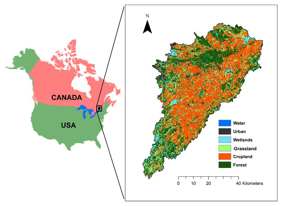
Figure 1 Location of the South Nation watershed (SNW) in North America. The inset figure (right) shows the land use distribution across the SNW.

2.2 Water balance quantification with HydroGeoSphere (HGS)

The water balance strongly influences ecosystem functions and the associated ecosystem services, as it governs both abiotic and biotic processes occurring within ecosystems (Mercado-bettín et al., 2019). Consequently, evaluating the role of water in ecosystem services' supply necessitates an analysis capable of water balance partitioning (i.e., disaggregation of the water balance into its fundamental components such as precipitation, subsurface evaporation, transpiration, surface and subsurface storages) (Casagrande et al., 2021). As HGS is a dynamic fully integrated subsurface–surface hydrologic model, it generates time-varying simulation outputs for all components of the terrestrial hydrologic cycle (Fig. 2), thus alleviating a common limitation of ecosystem services' models in that they do not account for transient behaviour (Vigerstol and Aukema, 2011). HGS employs a physically based approach to simulate water movement and the partitioning of precipitation input into surface runoff, streamflow, evaporation, transpiration, groundwater recharge, as well as groundwater discharge into surface water bodies like rivers and lakes (Brunner and Simmons, 2012). Furthermore, HGS outputs can also be generated for the entire model domain (i.e., the watershed) or refined for smaller spatial scales such as subwatersheds, with the downscale limit being that of an individual finite element within the finite element mesh (FEM).

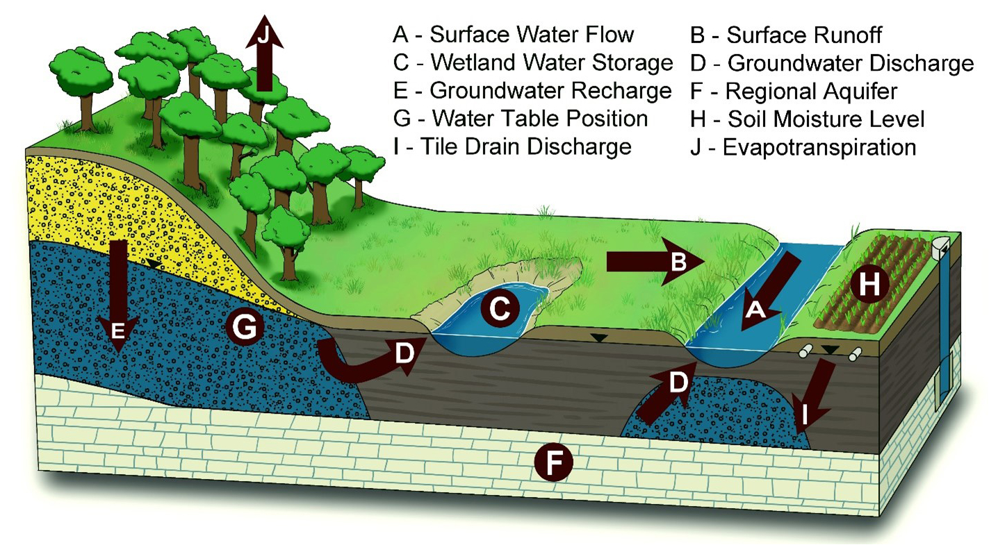
Figure 2 Key components of the terrestrial hydrological cycle captured in HGS models over a range of spatial scales.

It should be noted that the fidelity of the HGS outputs is also dependent on the model scale, with large-scale models generally having lower spatial resolution than small-scale models as a result of computational constraints, and in some cases, data constraints. For example, a model of a 766 000 km² river basin (e.g., Xu et al., 2021) is best suited to answer big picture questions (i.e., basin water balance), while a model built at similar scale to the SNW (e.g., Frey et al., 2021) can be used to address questions pertaining to more localized processes (i.e., individual wetland influences, groundwater recharge and discharge patterns, aquifer conditions, and soil moisture conditions). If even more localized insights are required, HGS models can be constructed for field- or plot-scale domains (up to approximately 10 km²), where questions pertaining to things such as riparian zones, soil structure, manure application, and tile drainage influences on both water quantity and quality can be evaluated (Fig. 2). Thus, HGS is a scalable and robust model for ecosystem services' analysis across a range of different spatial scales and different levels of hydrologic process detail. For the SNW, HGS is used to simulate watershed surface water outflow, transpiration (green water), subsurface water storage, and land-surface water storage (reflecting water held in wetlands and reservoirs) using the model construction framework presented in Frey et al. (2021).

2.2.1 Model construction

Finite element mesh (FEM)

The HGS model utilizes a 3-D unstructured FEM that extends across the full 3830 km² area of the SNW. The 1-D river/stream channel features, 2-D overland flow domain (reflecting land-surface topography), and 3-D subsurface flow domain (reflecting hydrostratigraphy) all share the same mesh geometry, with the 1-D and 2-D domains sharing common coordinates with the 3-D domain across the top surface of the model. The FEM for the SNW model resolves all Strahler 2+ stream/river features as mesh discretization control lines, with element edge length maintained at 125 m, while away from the control lines the element edge lengths extend up to 375 m. The FEM contains layer surfaces that correspond to hydrostratigraphic surfaces, with each individual layer consisting of 171 609 finite elements. Accordingly, over the eight model surfaces (seven subsurface layers); the FEM contains 1 201 263 three-dimensional finite elements.

Hydrostratigraphy

The seven subsurface layers represent (from the top down) three soil layers, three Quaternary hydrostratigraphic layers, and one bedrock layer. The soil layers extend from 0–0.25, 0.25–0.5, and 0.5–1 m depth relative to the top surface, which is defined with the Ontario Integrated Hydrology Data digital elevation model (https://geohub.lio.gov.on.ca/maps/mnrf::ontario-integrated-hydrology-oih-data/about, last access: 24 February 2025). The hydraulic properties for the soil layers vary spatially according to the soil polygons defined in the Soil Landscapes of Canada (SLC, 2010), and they are defined in two steps as follows: (1) properties extracted from SLC are used in conjunction with the Rosetta pedotransfer functions (Schaap et al., 2001) to obtain estimates for hydraulic conductivity, water retention, relative permeability, residual saturation, and porosity parameters; and (2) hydraulic conductivity, water retention, and relative permeability parameters are subsequently tuned during model calibration. The three Quaternary layers are of variable thickness, where the interface surfaces represent lithology contrasts derived from a simplified version of the 3-D geological model produced for the SNW by Logan et al. (2009). Hydraulic properties for the Quaternary materials are assigned based on lithology. Underlying the Quaternary layers is a single hydrostratigraphic layer with uniform hydraulic conductivity representative of the Phanerozoic bedrock. When assembled, the model layers depict a 3-D subsurface realization of the SNW hydrostratigraphy (Fig. 3).

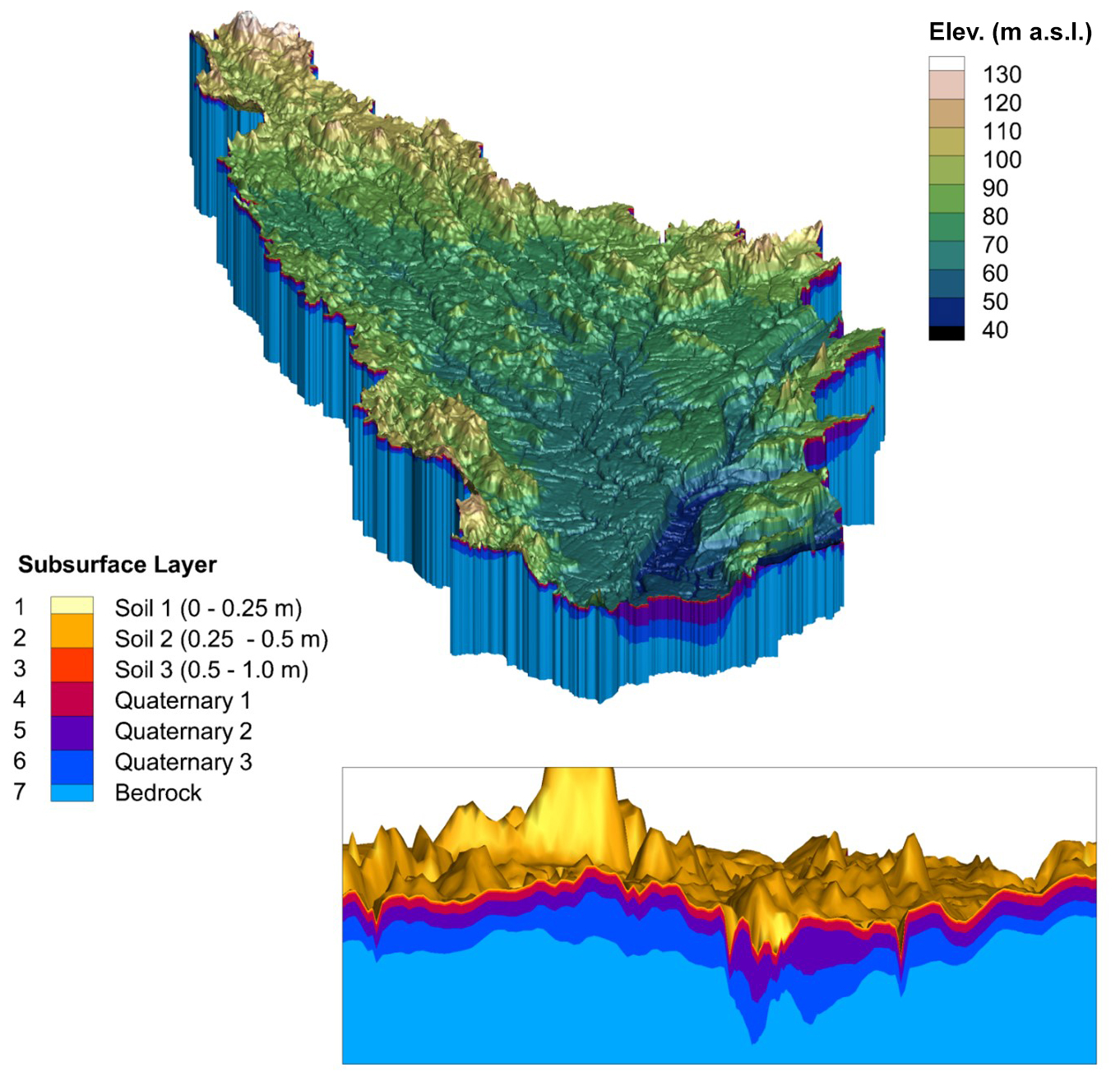
Figure 3 Three-dimensional perspective of the South Nation HydroGeoSphere model, and the hydrostratigraphic layering (inset). Note the 100× vertical exaggeration.

Land-surface configuration

The land surface in the HGS model represents the land cover distribution defined by the gridded, 30 m resolution, 2017 Annual Crop Inventory dataset (Agriculture and Agri-Food Canada, 2017) simplified to six categories (water, urban, wetland, grassland, cropland, and forest). Root depth for the cropland (1 m), forest (2.9 m), wetland (1 m), grassland (2.1 m), and urban (1 m) land covers was held static over the simulation interval. Spatially distributed leaf area index (LAI) is a transient parameter defined with the 8 d composite, 500 m resolution MOD15A2H v006 data product (Myneni et al., 2015). Each land cover category utilizes a unique surface roughness (Manning's n coefficient) value, ranging from 0.001 (urban) to 0.03 s m${}^{-\mathrm{1}/\mathrm{3}}$ (forest). Land cover properties, as well as subsurface hydraulic properties, were mapped into the HGS model's unstructured FEM using a dominant component approach, such that when two or more property classes exist within the input data set for a single finite element, the majority class is represented.

Climatology

Time-varying and spatially distributed climate data with daily temporal resolution liquid water influx (LWF) and potential evapotranspiration (PET) are used to force the HGS model for the 2000 to 2017 simulation interval. LWF is derived from precipitation obtained from McKenney et al. (2011) in combination with snow water equivalent (SWE) estimates from the ERA5-Land land-surface reanalysis (Muñoz-Sabater et al., 2021), where LWF is the sum of liquid precipitation (rain) and snowmelt (daily changes in SWE).

Potential evapotranspiration primarily depends on the surface radiation budget, temperature, humidity, and near-surface wind speed (Allen et al., 1998); however, of these variables, only minimum and maximum temperature are readily available for the full SNW. Hence, PET forcing for the SNW model is calculated with the Hogg method (Hogg, 1997), which is consistent with Erler et al. (2019) and Xu et al. (2021), who both reported good agreement with the observed water balance in the Great Lakes region when using the Hogg method. The Hogg method is based on the FAO Penman–Monteith approach (Allen et al., 1998) with a simplification that involves the radiation budget and humidity approximated as a function of daily minimum and maximum temperature, and wind speed is assumed to be constant.

2.2.2 Model performance evaluation

The SNW HGS model was run continuously for the 2000–2017 period with daily-temporal-resolution climate forcing, and simulation performance was evaluated using observed surface water flow rates and groundwater levels. The observation data are derived from daily-temporal-resolution surface water flow monitoring conducted at nine Water Survey of Canada (WSC) hydrometric stations (Fig. 4a) and groundwater level data from 10 Provincial Groundwater Monitoring Network wells that were measured hourly but aggregated into daily average values (Fig. 4b). The Nash–Sutcliffe efficiency (NSE) and percent bias (PBias) metrics (Moriasi et al., 2007) were used to evaluate surface water flow simulation performance, while the coefficient of determination (R²) and root-mean-square error (RMSE) were used to evaluate groundwater simulation performance. It should be noted that groundwater pumping was not represented in the model as it was deemed to be a very minor component of the overall water balance, and because it is extremely difficult to characterize and simulate at the scale of the SNW.

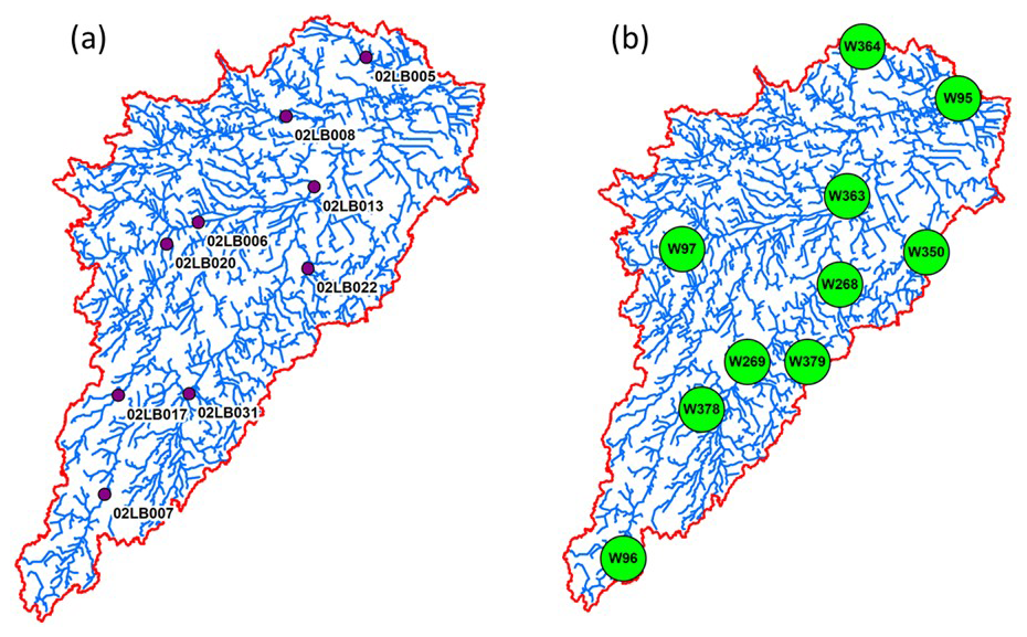
Figure 4 Distribution of (a) Water Survey of Canada surface water flow gauges, and (b) Provincial Groundwater Monitoring Network wells across the South Nation watershed.

2.3 Ecosystem services' water productivity

The benefit transfer method is used to derive the unit values of ecosystems in the SNW. The benefit transfer method, which is a widely used technique for assessing the economic value of ecosystem services, relies on secondary data obtained through the implementation of various other economic valuation methods (Aziz, 2021) and leverages existing valuation studies to estimate the value of the services in different geographical contexts. The method relies on two key assumptions. First, it assumes that the value of any ecosystem service (or bundle) under valuation is comparable across different regions, which may not always hold true due to variations in ecological and socio-economic conditions. Additionally, the methods used in the primary studies (e.g., market price, replacement cost methods) assume that market prices or the costs of replacing ecosystem services accurately reflect their true value (Aziz et al., 2023). These assumptions inherently limit the precision of the results, meaning the estimated values should be interpreted as approximate rather than definitive. Nevertheless, these estimates provide useful insights, especially for regions like the South Nation watershed, where primary valuation studies are lacking and can guide initial policy development and resource management decisions.

A study conducted approximately 65 km from the SNW in the Ottawa–Gatineau region, by L'Ecuyer-Sauvageau et al. (2021), assembles the values for 13 ecosystem services: agricultural services, global climate regulation, air quality, water provision, waste treatment, erosion control, pollination, habitat for biodiversity, natural hazard prevention, pest management, nutrient cycling, landscape aesthetics, and recreational activities. These 13 ecosystem services are the focus of the present analysis and their unit values have been correspondingly generated by major ecosystems using market price, replacement cost, and benefit transfer methods. The unit values for ecosystem services are based on similarities in ecologic and socio-economic conditions between the studied and policy sites, and they were converted using the purchasing power parity (L'Ecuyer-Sauvageau et al., 2021). The benefit transfer method provides an approximation of ecosystem service values with potential transfer errors ranging from 62 % to 86 % based on domestic studies (Aziz, 2021). In our study context, we transfer the values from the region immediately adjacent to our study region, an approach that constrains the error. After adjusting these values for inflation, the value of ecosystem services in the SNW is calculated using the following equation.

$$\begin{array}{}\text{(1)}& {\mathrm{EV}}_t=\sum _{k=\mathrm{1}}^n\left(A_k\times {\mathrm{UV}}_k\right)\times VI\end{array}$$

EV_t represents the value of ecosystem services for year t, A_k represents the area of land use k, UV_k represents the unit value of ecosystem services for land use k, and VI represents the vegetation indicator – a ratio of yearly to average net primary production (NPP) (where NPP = NPP_year/NPP_mean).

We use net primary production as an indicator to characterize the vegetation vigour (Xu et al., 2012) and to adjust the values of ecosystem services over time in the SNW. The Moderate Resolution Imaging Spectroradiometer (MODIS) (https://appeears.earthdatacloud.nasa.gov/, last access: 24 February 2025) NPP data (at 500 m resolution) for the 2000 to 2017 study period are used (Fig. A5). Using the ArcGIS Spatial Analyst toolbox, yearly mean NPP values are calculated. The average ecosystem services' water productivity is then calculated using ecosystem services' values and productive green water volumes (i.e., transpiration) in Eq. 2:

$$\begin{array}{}\text{(2)}& V_{Wt}=\left({\mathrm{EV}}_t\right)/\left(X_{wt}\right),\end{array}$$

where V_wt is the average product of water (CAD m⁻³), and X_wt is the total volume of water transpired (or volume of green water used for transpiration) in year t.

2.4 Valuation of the subsurface water contribution towards ecosystem services' supply

A water production function is developed using economic values of the supply of the 13 watershed ecosystem services over the 18-year study period and corresponding volumes of green water used by plants for transpiration. Because ecosystem services' value is proportional to vegetative biomass production (Costanza et al., 1998), the values are modified over time using relative changes in ecosystem vegetative biomass in the watershed (Xu and Xiao, 2022). The slope of the production function represents the ecosystem services' marginal water productivity (MP_w). HGS model outputs capture the volume of subsurface water contributing to transpiration. Using transpired water volume and MP_w, the economic value of green water is calculated (Eq.3).

$$\begin{array}{}\text{(3)}& V_t=X_{wt}\times {\mathrm{MP}}_{\mathrm{w}}\end{array}$$

where V_t is the value of subsurface water used towards ecosystem services' supply, X_wt is the volume of subsurface water transpired or productive green water volume in year t, and MP_w is the marginal productivity of water.

3 Results

3.1 HGS outputs

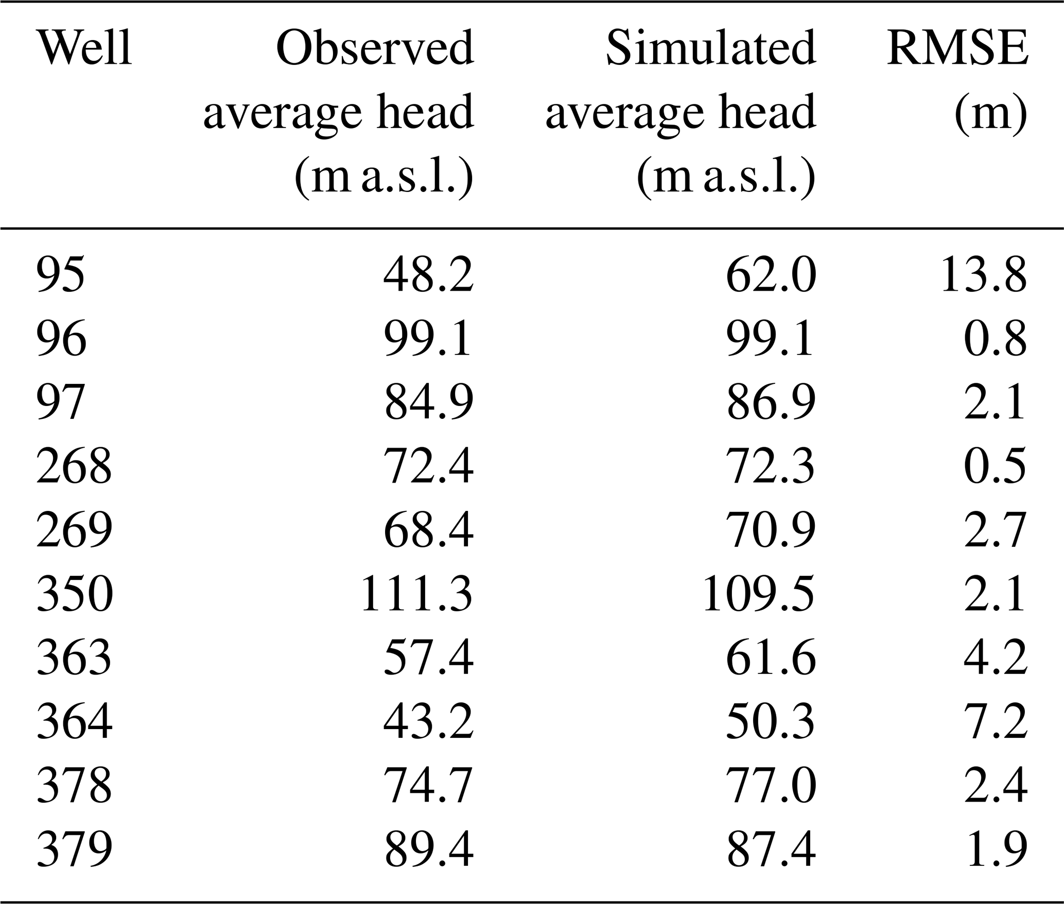
For the 2000 to 2017 simulation interval, the HGS model reproduces surface water flow rates at the nine WSC hydrometric stations across the SNW with good accuracy as per the interpretation guidance provided by Moriasi et al. (2007). Based on daily evaluation frequency, NSE at the individual gauge stations ranges from 0.60 to 0.72, with a mean of 0.66, while PBias ranges from −15.3 % to 16.0 %, with a mean of 3.6 % (Fig. 5). Groundwater levels were also reproduced across the SNW with reasonable accuracy for the 2000 to 2017 interval. The R² between simulated and observed water levels in the 10 observation wells is 0.98, with the simulated values having a mean value 2.8 m higher than the observed values. Groundwater simulation performance at the individual wells is presented in Table 2. HGS outputs (Fig. 6) also include total watershed surface water outflow, ET_a rates (based on subsurface transpiration and evaporation, surface evaporation, and canopy evaporation), subsurface water storage (groundwater storage plus soil moisture storage), and land-surface water storage. During the simulation period, transpiration accounts for a substantial proportion of ET_a, ranging from 45 % to 65 % (Table A1). Consequently, it emerges as the dominant process contributing to the overall ET_a. As evident in Fig. 6, water storage volumes fluctuate over inter- and intra-annual time frames, with the most notable decline in storage aligned closely with the drought in 2012.

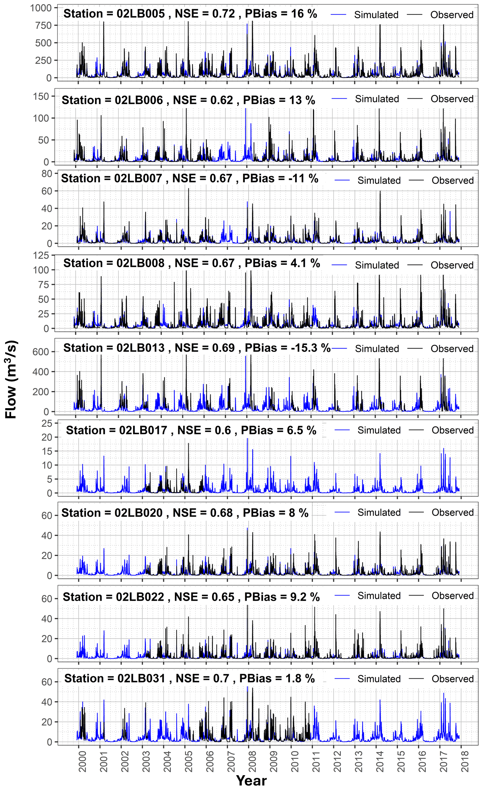
Figure 5 Simulated vs. observed surface water flow rates at the nine Water Survey of Canada (WSC) flow gauges incorporated into the model calibration process, along with Nash–Sutcliffe efficiency (NSE) and percent bias (PBias in %) performance metrics. Note that not all gauges have a full data record over the 18-year simulation interval.

Table 1 Land use types and unit values of ecosystem services for the SNW.

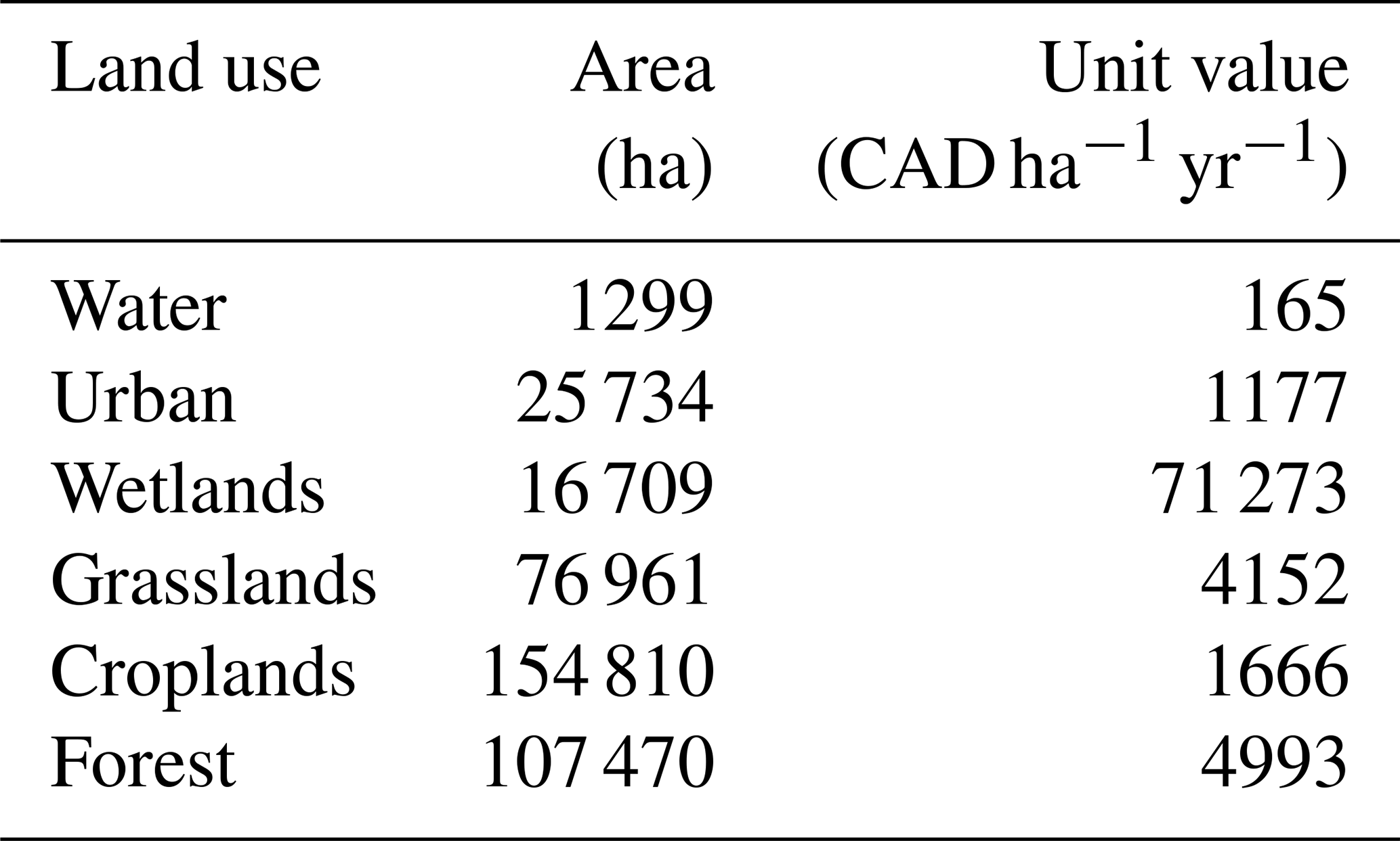
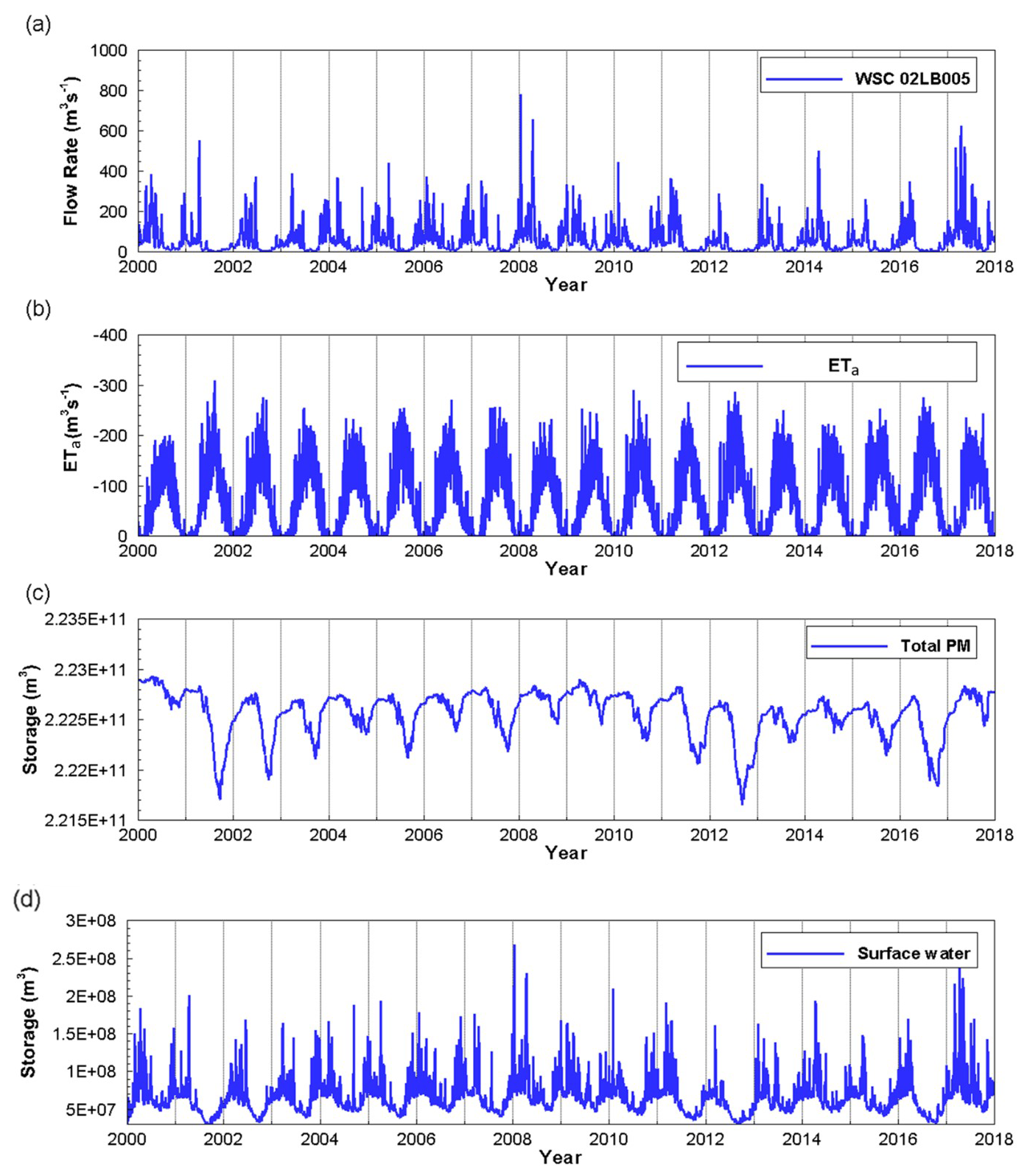
Figure 6 Time series outputs from the South Nation watershed HydroGeoSphere (HGS) simulation over the 2000-to-2017 time interval. (a) Stream flow at the furthest downstream hydrometric station, (b) watershed evapotranspiration, (c) watershed subsurface water storage, and (d) watershed land-surface water storage.

The HGS output was generated at variable time steps that were each no larger than 1 d and then aggregated to yearly values for use in the ecosystem services' assessment (Table A1). Annual deviations from the long-term mean (for ET_a, transpiration, total precipitation, and surface and subsurface water storage) are presented in Fig. 7. In the context of subsequent analysis and discussion, it should be noted that the drought year of 2012 exhibits the highest ET_a and transpiration, lowest precipitation, and largest relative drops in both subsurface and surface water storage.

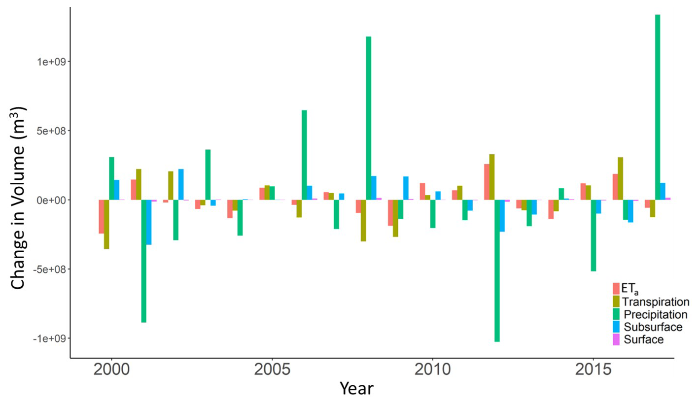
Figure 7 Annual deviation from the long-term (2000–2017) mean evapotranspiration (ET_a), transpiration, precipitation, and subsurface and surface water storages.

Table 2 For the 10 monitoring well locations, observed vs. simulated average groundwater head and root-mean-square error between daily temporal resolution observed and simulated head data over the 2000–2017 simulation interval.

3.2 Valuation of ecosystem services and average and marginal water productivity

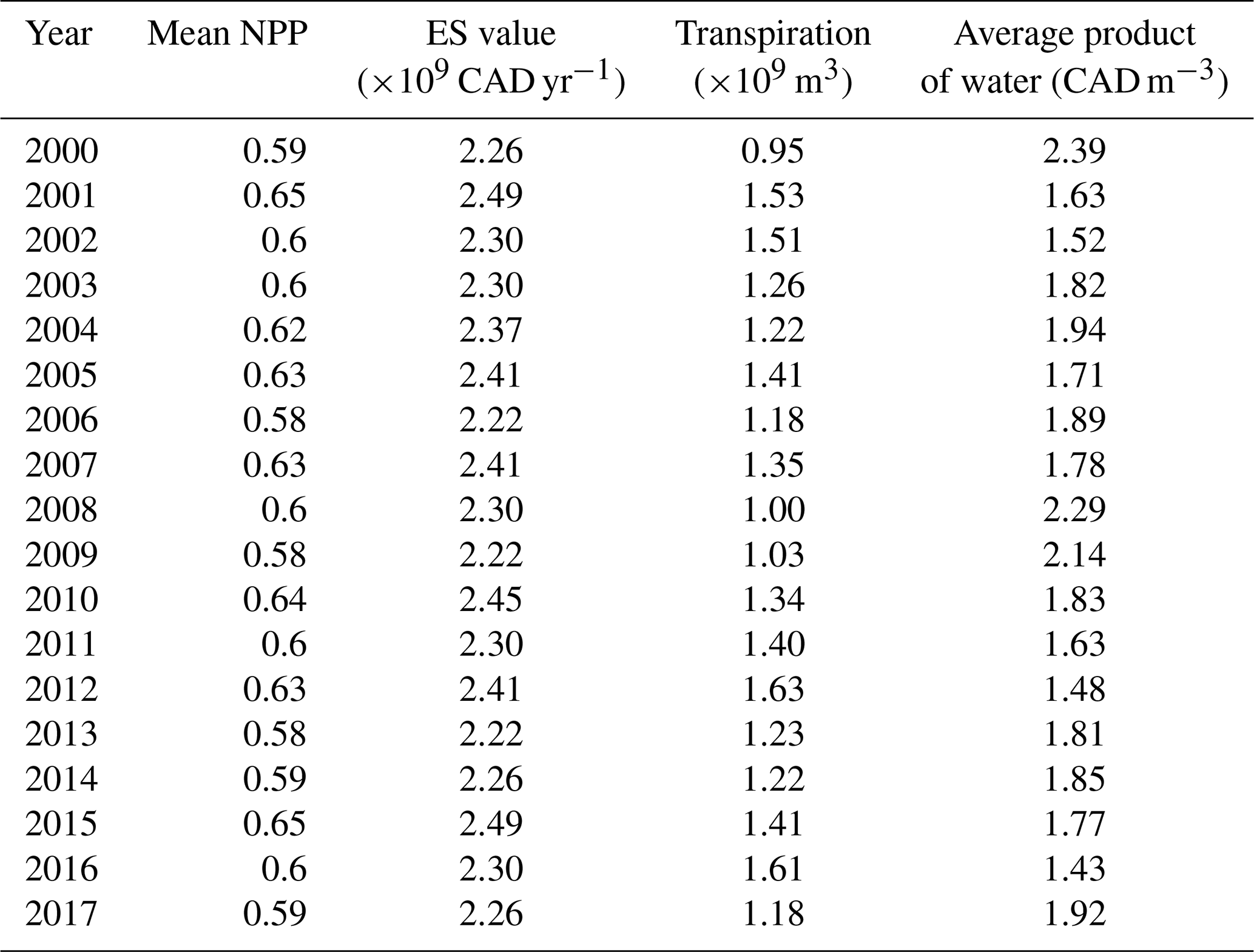
Using unit values for the major land use types in the SNW (Table 1) and land use area, the total value of the 13 ecosystem services under consideration is CAD 2.33 billion yr⁻¹ (in CAD 2022) prior to further annual modifications based on the vegetation indicator (Eq. 1). The estimates for average product of water are point estimates based on the value of ecosystem services and productive green water volume (i.e., transpiration) for the corresponding year. Annual NPP data (rescaled between 0 and 1), ES values, transpiration volume, and average water product in the SNW are given in Table 3.

Table 3 Mean net primary production (NPP), ecosystem services' (ES) values, transpiration volume, and average product of water for the SNW over the 18-year study interval.

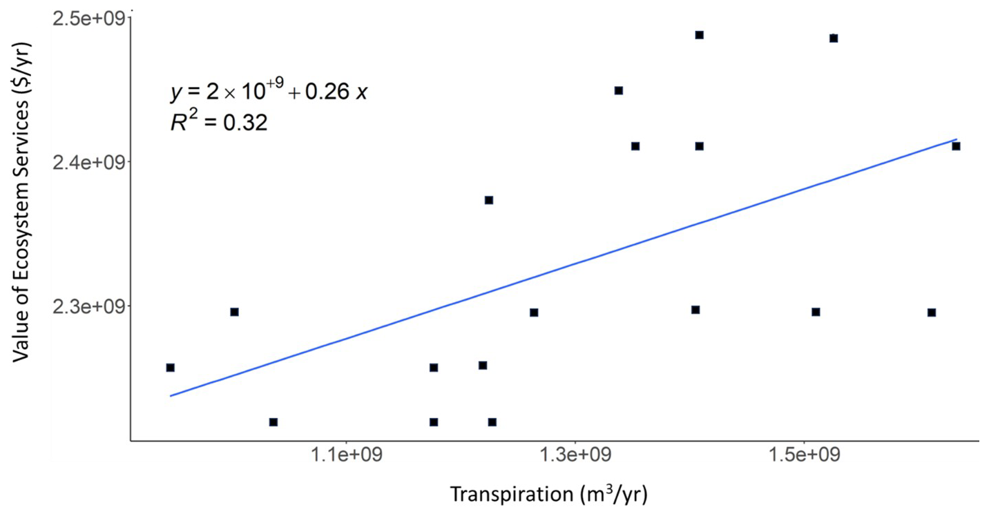
For the ecosystem services' marginal water productivity, a production function is developed using transpiration and ecosystem services' values for the SNW (Fig. 8) and the slope of the function equates to the marginal productivity of water, which is CAD 0.26 m⁻³.

Figure 8 Ecosystem services' water production function for the SNW.

To assess the contribution of subsurface water towards ecosystem services, the average ecosystem services' water productivity at the watershed scale is calculated (Table 3). The average product of water over the 18-year study interval ranges from CAD 1.43–2.39 m⁻³ (Fig. 9). During the drier years (2001–2002, 2012, and 2016), the average product of water declines to local minima. This is because the average product depicts water use efficiency, with the highest value observed for the year 2000, indicating that hydrologic conditions favoured the maximum production of ecosystem services with the lowest water consumption in that year.

3.3 Valuation of green water

Using the marginal water productivity and transpiration in the SNW, the value of the productive green water (i.e., subsurface water) over the study period was calculated (Fig. 10). The annual values range from CAD 245.9 million per year (year 2000) to CAD 424.7 million per year (year 2012) , with an overall average of CAD 338.83 million. In the SNW, precipitation is the main driver of the terrestrial hydrologic cycle and low precipitation is the primary indicator of climatological drought. In general, there is a strong inverse correlation between total annual precipitation and green water value, with an R² of 0.45 (p<0.0001).

4 Discussion

4.1 Drought year hydrologic behaviour

In this study, HGS is used to capture the contributions of subsurface water storage to transpiration (i.e., productive green water) and quantify its role in sustaining transpiration and subsequent ecosystem services.

The annual deviations from the long-term means (Fig. 7) show that ET_a and transpiration are supported by the subsurface and surface storages during droughts. In the drought period from 2001–2002, an interesting situation arises. In 2001, both ET_a and transpiration exhibit positive values relative to the mean. However, in 2002, despite ET_a being negative, transpiration remains positive and surpasses the mean value. This deviation can be attributed to the diminished availability of surface water, leading to reduced evaporation and subsequently lower ET_a. Nevertheless, transpiration continues to exceed the average due to its reliance on subsurface water availability within the SNW. This finding is further supported by previous studies, which suggest that transpiration dominates ET_a during drought years, while evaporation takes precedence during wet years (Zhang et al., 2019). To further compare the fluctuations in different storage zones on a common scale, the standard scores (that is, the change in a storage/standard deviation) for each zone are calculated over time (Fig. 11). The standard scores show that ET_a is supported by both surface and subsurface water storages during the dry periods. However, the contribution of subsurface water by volume during drought is much larger than that of surface water, thus highlighting the important role of subsurface water in supporting transpiring biota during droughts.

Comparison of years 2001 and 2012 (both with less precipitation than the 18-year mean) shows that the ET_a was less but outflow was more in 2001 relative to 2012 (Fig. 6a). In such case, it is the subsurface water contribution in 2001 that maintained the higher surface water flows, which highlights the important role of antecedent conditions in regulating low flow response. Nevertheless, the influence of subsurface water on consumptive water use also depends on the timing of precipitation along with other climatic conditions (temperature, atmospheric moisture demand, etc.) in the corresponding years (Zhao et al., 2022). During drought periods, vegetation and atmospheric moisture demand is often not met, thus resulting in ecosystem stress along with depletion of subsurface and surface water storages (Zhao et al., 2022). Given the complexities involved with linking transpiration with subsurface water storages, full characterization of transpiration influences on ecosystem services during droughts has until now received little attention.

The study quantifies subsurface water ecosystem services' values, at the scale of a 3830 km² watershed, over a period that encompasses a wide range of climatological conditions. Previous studies (e.g., Loheide, 2008; Su et al., 2022) have estimated groundwater contribution to evapotranspiration by linking water table fluctuation with changes in evapotranspiration. However, over large areas, using water table fluctuation can be complicated by other subsurface water sinks, including deeper groundwater recharge and discharge into surface water receptors. With the HGS approach employed herein, the computed subsurface water evaporation and transpiration, and surface water evaporation, in conjunction with the other hydrologic flow processes depicted in Fig. 2, provides a physically based numeric characterization of water storage contributions to ET_a.

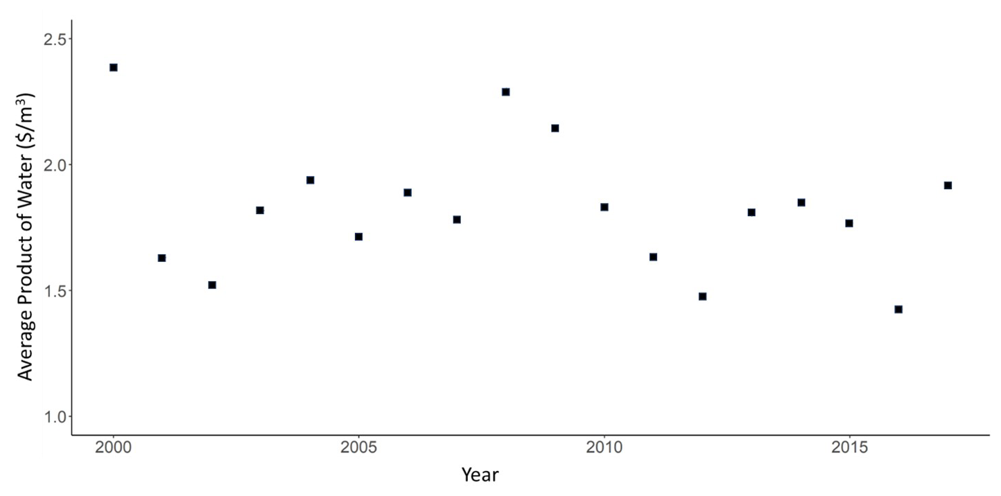
Figure 9 Average annual product of water (Table 3) for ecosystem services in the SNW over the 18-year study period.

Figure 10 Value of productive green water in the SNW over the 18-year study period.

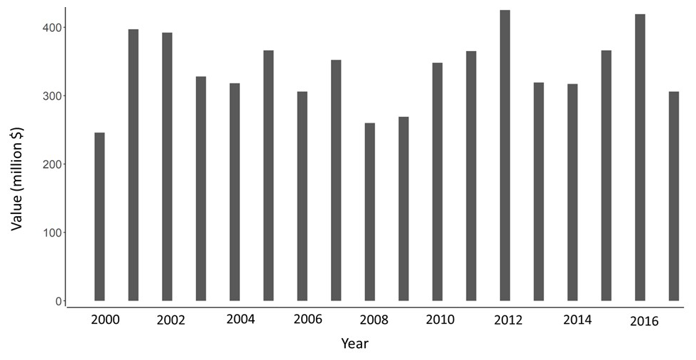
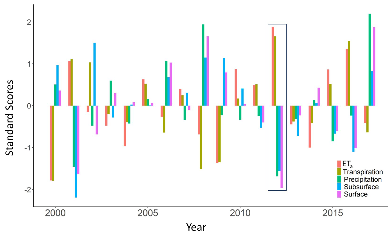
Figure 11 Change in standard scores of water storages/hydrological variables over the 18-year study period. The scores for the 2012 drought year are bordered.

The fluctuations in water storages show that, in general and with respect to longer-term mean conditions, subsurface water storage replenishes when ET_a is negative and depletes when ET_a is positive. In both the 2001 and 2012 drought years, ET_a is relatively high in comparison to the wet years with high precipitation. ET_a in drought years is primarily supported by the drawdown (by volume) in subsurface water storage below the mean level. In general, fluctuations in subsurface water storage across the 18 years are congruent with changes in precipitation, with above-average precipitation aligned with increases in subsurface water storage and vice versa. In contrast, increased ET_a leads to a reduction in subsurface storage and vice versa. Over the 18-year study period, the maximum increase in subsurface water storage occurred in the year 2002, immediately following the 2001 drought which had implications far beyond just the SNW (Wheaton et al., 2008). Even though 2002 was a year with less than average precipitation, the drought-impacted subsurface storage conditions led to an antecedent condition across the SNW that was favourable for subsurface water recharge.

4.2 Hydrologic influences on ecosystem services and economic valuation

Based on this study, fully integrated groundwater–surface-water models, such as HGS, have the potential to facilitate better management of watershed-scale (approximately 4000 km²) water resources for ecosystem services' endpoints and to help determine the role of a range of water resources that sustain green water supply. A water production function was developed using total green water volumes and total values of 13 ecosystem services in the SNW: agricultural services (net benefits from the crops or agricultural products), global climate regulation, air quality, water provision, waste treatment, erosion control, pollination, habitat for biodiversity, natural hazard prevention, pest management, nutrient cycling, landscape aesthetics, and recreational activities. The ecosystem water production function yields a marginal value of CAD 0.26 m⁻³ of green water devoted to transpiration (Fig. 8). Globally, Lowe et al. (2022) estimated the average marginal product of water specifically for crop production at CAD 0.083 m⁻³. While water productivity is greatest when the smallest amount of water is used/consumed, it also produces the smallest value of ecosystem services at this point. Between 2000 and 2017, transpiration in the SNW is highest during the driest years (Zhao et al., 2022). The NPP does not decline during these periods, likely due to enough subsurface water to meet plant demands (e.g., Hosen et al., 2019; Sun et al., 2016). Modelling results presented herein show that the dry meteorological conditions are associated with relatively higher transpiration and ET_a rates, similar to Zhao et al. (2022) and Diao et al. (2021). During dry years, the increase in transpiration is positively correlated with higher NPP, which in turn relates to lower relative ecosystem service water productivity values (Fig. 9).

In the SNW, green water use is higher in years with less-than-average precipitation. Accordingly, the green water value was highest, at CAD 424.7 million (in CAD 2022), for the 2012 drought year (Fig. 10). It is important to note that value of the subsurface water contribution is second highest, at CAD 418.63 million, for 2016, which is also a drought year. Hence, the critical role of subsurface water in sustaining ecosystem services is especially evident during both drought years and more typical climatic conditions.

4.3 Strengths and limitations of fully integrated groundwater–surface-water models

While this study advances the scientific utility of physics-based fully integrated groundwater–surface-water models, it is essential to acknowledge the inherent uncertainty associated with such an analysis, along with factors that could potentially reduce this uncertainty. It is well known that highly parameterized, structurally complex models can have many degrees of freedom, high data requirements, and non-uniqueness challenges (Beven, 2006). However, the parameterization of physics-based models can also be viewed as a strength due to the constraining relationship between physically measurable characteristics and parameter values (Ebel and Loague, 2006). For the SNW, soil and subsurface materials are well characterized; hence, the spatial distribution and magnitudes of the associated hydraulic parameters are generally well represented in the HGS model. Incorporating meteorological variability into structurally complex model calibration and performance evaluation can also act to reduce uncertainty (Moeck et al., 2018). Because the SNW simulation extended over an 18-year time frame that included multiple droughts and floods, there is confidence that the model structure and parameterization is suited for a wide spectrum of hydrologic conditions and that the model can dynamically capture transitions from wet-to-dry and dry-to-wet conditions, which is a critical part of the SNW analysis.

Fully integrated groundwater–surface-water models are ideally suited for the type of challenge addressed in the work herein because simpler models lack process representation critical within the problem conceptualization (Ebel and Loague, 2006). This is especially true when considering difficulties associated with quantifying large-scale evaporation and transpiration fluxes (Stoy et al., 2019), as well as groundwater–surface-water interactions (Barthel and Banzhaf, 2016). Structurally complex models have been shown to perform better than simple models when simulating evapotranspiration (Ghasemizade et al., 2015) and groundwater recharge (Moeck et al., 2018), and previous work by Hwang et al. (2015) demonstrated the utility of HGS for constraining ET at the watershed scale within the same geographic region as the SNW. Further confidence in the SNW HGS model can be established through comparison with other studies. In terms of overall water balance, results from this study compare closely with data compiled as part of a regional water management study encompassing the SNW (EOWRMS, 2001). Although the study time frames differ (the EOWRMS 2001 study utilized pre-2000 data), the results are similar, with ET_a accounting for approximately 45 % and 62 % of annual precipitation in EOWRMS (2001) and this study, respectively. While there is limited previous work investigating the partitioning of ET_a into transpiration and evaporation that can be directly compared, it is useful to refer to a highly detailed analysis based off FLUXNET data (Pastorello et al., 2020) as a reference for transpiration and evaporation partitioning in land cover settings representative of those within the SNW. For example, Xue et al. (2023) reported that transpiration as a percentage of ET ranged (depending on calculation method) from 21 %–56 % and 39 %–83 % in FLUXNET data from cropland and mixed forest settings, respectively, whereas the HGS model predicts an aggregate range of 45 %–65 % across the SNW watershed, which supports the use of HGS transpiration estimates in subsequent ecosystem services' valuation.

4.4 Extension to other regions

The methodology employed in this study provides a basis for deploying fully integrated groundwater–surface-water models to assess the subsurface water contribution to ecosystem services in other regions. However, it must be noted that the results and values used herein are not necessarily transferable to other sites/watersheds. The marginal product of water is a site-specific entity that will be different for other watersheds because both ecosystem services' value and transpiration rate will change in response to factors such as land cover, NPP, climate/weather, hydrogeology, and soil properties. Nevertheless, given the ability of fully integrated models to quantify the dynamic fluctuation in water storages across different compartments, along with the linkage to terrestrial ecosystem services, the approach can be expected to yield reliable results under similar workflows (modelling of water storages and transpiration rates and valuation of ecosystem services) for other locations, sites, or watersheds.

5 Conclusions

This study characterizes and quantifies the important contribution of subsurface water towards sustaining ecosystem services, which, until now, have not been comprehensively studied. The prior lack of attention to subsurface water in part relates to the complexities involved with characterizing the dynamic movement of water between subsurface water and surface water storage compartments, and the related supply of green water. In the work herein, focusing on a 3830 km² mixed-use watershed, the innovative use of a HGS fully integrated groundwater–surface-water model for water ecosystem services' valuation is demonstrated, with the endpoint being monetization of the contributions of subsurface water to green water supply over a period of 18 years (2000–2017). Results show that droughty conditions are a major impetus for increased green water use. The maximum annual productive green water value was CAD 424.7 million (CAD 2022) during the 2012 drought year, while the 18-year average was CAD 338.83 million. Similarly, in other dry years (i.e., 2001–2002 and 2016), there was a discernible rise in the green water use. Conversely, the results show a notable decrease in the green water use during years characterized by higher precipitation, as exemplified in the year 2000 where green water provided CAD 245.9 million in ecosystem services' value. Hence, the study emphasizes the key role of subsurface water in supplying green water and sustaining ecosystem services during critical periods when the watershed is under meteorological drought.

Surface water ecosystem services are frequently valued in the literature, whereas the valuation of subsurface water reserves and flows receives considerably less attention. Valuing groundwater resources can provide watershed stewards incentives they can use to support land use management practices that influence flood damages, drought impacts, drinking water quality/quantity, and ecological functions in surface water systems, for instance. The valuation approach provided herein, using integrated numerical hydrogeological models, provides a rigorous standardized means to provision value to ecosystem services associated with all components of the hydrological cycle. This approach offers a template for standardizing water valuation in ecosystem service markets and could guide the integration of water ecosystem service payments across diverse jurisdictions.

Appendix A

The annual outputs (ET_a, surface water, subsurface water, precipitation and outflow) from the HGS model are given in Table A1.

Table A1 HGS outputs from the SNW simulation.

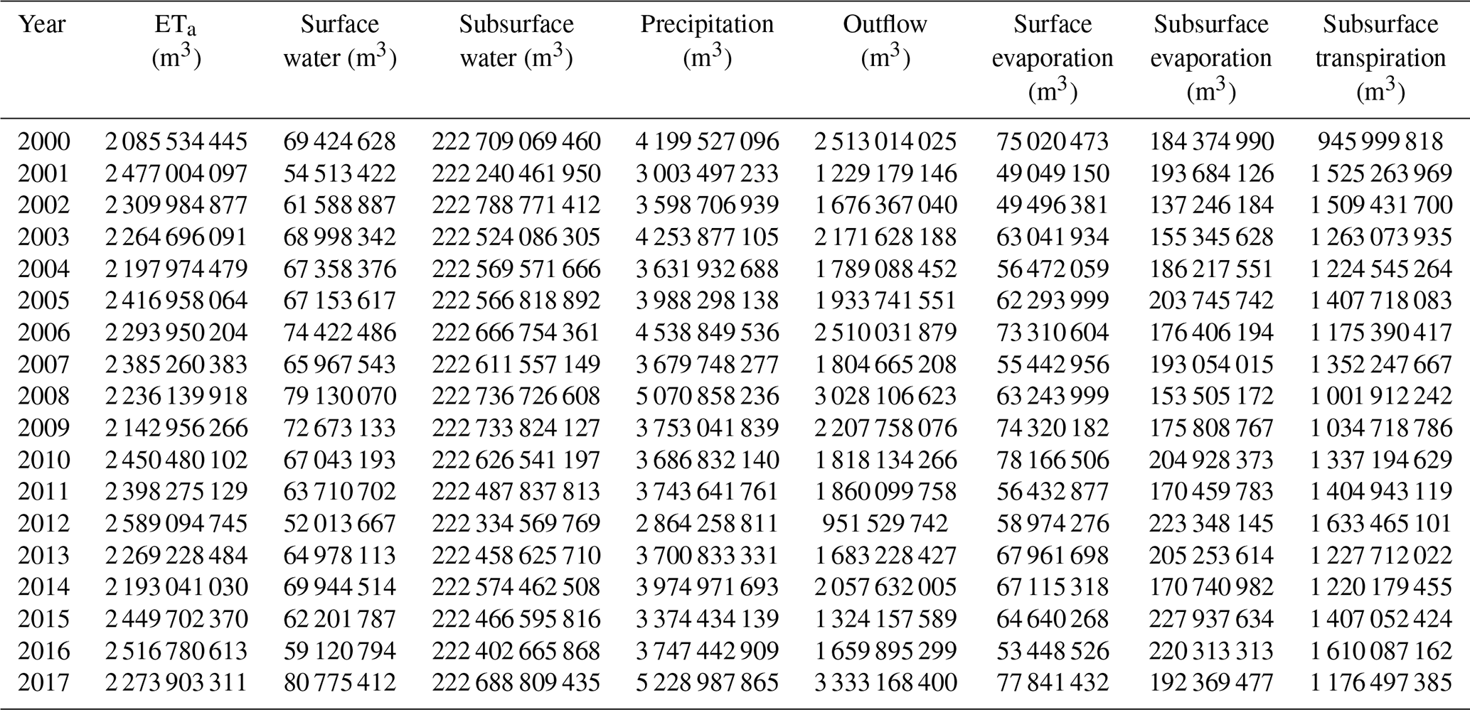
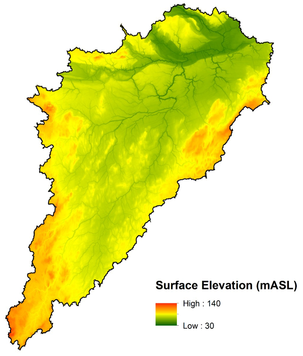
Figure A1 Land-surface elevation of the SNW (Ontario Integrated Hydrology Data).

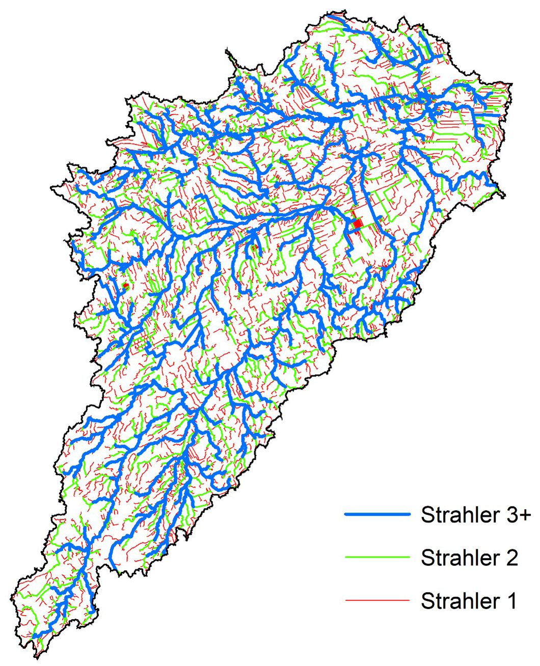
Figure A2 Stream network distribution across the South Nation watershed, consisting of 1606 km of Strahler 3+ streams, 1548 km of Strahler 2 streams, and 3335 km of Strahler 1 streams (Ontario Ministry of Natural Resources and Forestry 2013).

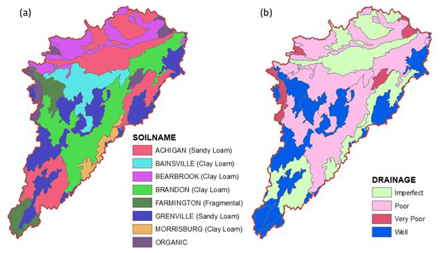
Figure A3 (a) Soil distribution and (b) soil drainage status across the South Nation watershed (SLC, 2010).

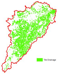
Figure A4 Tile drainage distribution across the South Nation watershed (data provided by the South Nation Conservation Authority).

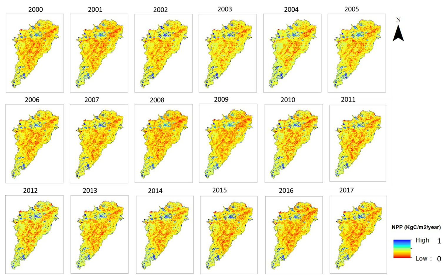
Figure A5 Net primary productivity (NPP) data for SNW (based on MODIS data; Endsley et al., 2023).