The significance of the leaf area index for evapotranspiration estimation in SWAT-T for characteristic land cover types of West Africa

Evapotranspiration (ET) is pivotal in the terrestrial water cycle in subhumid and tropical regions. In the water cycle, the contribution of plant transpiration can be distinctively more significant than soil evaporation. The seasonal dynamics of plant phenology, commonly represented as the vegetation attribute leaf area index (LAI), closely correlates with actual ET (AET). Hence, addressing the reciprocal LAI–AET interaction is essential for practitioners and researchers to comprehensively quantify the hydrological processes in water resources management, particularly in the perennially vegetated regions of West Africa. However, due to a lack of field measurements, evaluation of the LAI–AET interaction still remains challenging. Hence, our study aims to improve the understanding of the role of the LAI in AET estimation by investigating characteristic regions of West Africa. We set up ecohydrological models (using the Soil and Water Assessment Tool for the tropics – SWAT-T) for two homogeneous land cover types (forest and grassland) to guarantee the representativeness of field measurements for the LAI and AET. We apply different potential ET methods (the Hargreaves; Penman–Monteith – PET-PM; and Priestley–Taylor methods) to evaluate the LAI–AET interaction in SWAT-T. Further, the elementary effects method quantifies the parameter sensitivity for 27 relevant LAI–AET parameters. The comprehensive parameter set is then optimized using the shuffled complex evolution algorithm. Finally, we apply a benchmarking test to assess the performance of SWAT-T with respect to the simulation of AET and to determine the relevance of detailed LAI modeling. The results show that SWAT-T is capable of accurately predicting the LAI and AET at the footprint scale. While all three PET methods facilitate adequate modeling of the LAI and AET, the PET-PM technique outperforms the other methods for AET, independent of the land cover type. Moreover, the benchmarking highlights that, if it only accounts for the LAI but disregards AET data, an optimization process's prediction of AET still yields an adequate performance with SWAT-T for all PET methods and land cover types. Our findings demonstrate that the significance of detailed LAI modeling for the AET estimation is more pronounced in the forested than in the grassland region.

1 Introduction

Evapotranspiration (ET) is a key hydrological process of the continental water cycle, particularly in the subhumid and tropical regions of West Africa where the share of ET to precipitation can be up to 70 %–80 % (Rodell et al., 2015). The high share of ET in the water cycle inevitably necessitates the reliable estimation of ET for water resources studies at all scales in subhumid and tropical regions. Concurrently, the accurate computation of ET remains challenging for researchers and practitioners, as ET is dynamic in space and time (Michel et al., 2016; Miralles et al., 2016). Its variability notably depends on land cover, soil properties, water availability, vegetation state, and time of the year (Chu et al., 2021). In addition, plant transpiration has a decisive contribution to the total evapotranspiration (Gerten et al., 2004; Schlesinger and Jasechko, 2014; Miralles et al., 2016; Wei et al., 2017). It is directly linked to the canopy conductance, which strongly correlates with the leaf area index (LAI) (Good et al., 2014; Wang et al., 2014). Thus, in perennially vegetated regions with high transpiration rates, such as subhumid West Africa, the LAI–ET interaction plays a pivotal role in the ET quantification (Schlesinger and Jasechko, 2014; Wei et al., 2017; Bright et al., 2022).

Although important, the availability of LAI and ET ground measurements is scarce. In previous ET studies, authors have used existing global monitoring networks, such as eddy-covariance (EC) systems (e.g., AmeriFlux – Novick et al., 2018; AMMA-CATCH – Galle et al., 2018; or FLUXNET – Friend et al., 2007), to inform catchment-scale hydrological models to comprehensively assess all processes of the hydrological cycle (Schneider et al., 2007; Hector et al., 2018; do Nascimento Ferreira, 2021; Jepsen et al., 2021; López-Ramírez et al., 2021). Still, the derived actual ET (AET) estimates from EC systems can not be extrapolated beyond the location site without limitations. This is mainly attributed to the small footprint, i.e., the source area of the AET fluxes. Depending on soil and land cover properties underlying the footprints, the source area spatially limits the representativeness of the AET measurements (Chu et al., 2021). For the LAI, the limited availability of field observations is commonly addressed by exploiting satellite-based LAI data. An example of favorable satellite-based LAI information is the Global Land Surface Satellite (GLASS) data set (Liang et al., 2021), in which the widely used Moderate Resolution Imaging Spectroradiometer (MODIS) LAI data have been advanced with machine learning applications at the global scale (Liang et al., 2014). The validation reports of GLASS LAI data present accurate LAI time series results, particularly in perennially vegetated regions (Liang et al., 2014) where satellite-based vegetation data can be subject to noise and cloud influences (Viovy et al., 1992; Strauch and Volk, 2013; Atkinson et al., 2012; Alemayehu et al., 2017).

In the present study, the semi-distributed, physically based ecohydrological Soil and Water Assessment Tool for the tropics (SWAT-T) (Alemayehu et al., 2017) is applied. The SWAT-T model is a modification of SWAT (Arnold et al., 1998), which was introduced by Strauch and Volk (2013) and further developed by Alemayehu et al. (2017) to account for more realistic plant growth modeling of perennial vegetation in tropical regions. The merits of SWAT-T for the improved prediction of the LAI and AET have been highlighted in different tropical and subhumid regions. It has been applied at the catchment scale in East Africa (Alemayehu et al., 2017), Colombia (Hoyos et al., 2019), Brazil (do Nascimento Ferreira, 2021), and Australia (Zhang et al., 2020) a well as at the micro-catchment scale in Mexico (López-Ramírez et al., 2021). Moreover, the application of SWAT-T for climate impact assessment has been presented in Peru at the catchment scale (Fernandez-Palomino et al., 2021). Remotely sensed AET has been chiefly employed to assess the model fitness of simulated AET with SWAT-T (Alemayehu et al., 2017; Zhang et al., 2020; Fernandez-Palomino et al., 2021; do Nascimento Ferreira, 2021) as well as with SWAT (Rajib et al., 2018; Qiao et al., 2022). The latest, open-source version of SWAT, called SWAT+, has also been applied in the tropics with remotely sensed AET and LAI data (Abitew et al., 2023). For the African continent, remotely sensed AET products can be limited due to uncertainties in their reliability (Weerasinghe et al., 2020).

For LAI estimation, the SWAT-T studies mentioned above relied on the application of remotely sensed LAI information from MODIS, e.g., by Alemayehu et al. (2017). Measured data for the modeling of vegetation, e.g., measured LAI (Park et al., 2017; Yang et al., 2018; Nantasaksiri et al., 2021; Haas et al., 2022) or observed forest biomass production (Khanal and Parajuli, 2014; Haas et al., 2022) has also been used to assess the LAI modeling ability of SWAT. However, the number of parameters used in prior studies has differed, e.g., the total number of parameters applied ranges from 3 (Yang et al., 2018) to 18 (Haas et al., 2022). For tropical regions, Alemayehu et al. (2017) suggest the calibration of 11 LAI parameters when SWAT-T is applied. The LAI and AET are correlated and influence each other in SWAT/SWAT-T (Arnold et al., 1998). For example, the water stress on plants is dependent on AET and can determine the actual plant growth in SWAT/SWAT-T (Neitsch et al., 2011). Therefore, when modeling the LAI, the relevant AET parameters must be considered.

To the best of our knowledge, the integration of measured LAI and AET data in the evaluation of the reciprocal LAI–AET interaction and the relevance of a coupled LAI–AET parameter estimation with the SWAT/SWAT-T model has yet to be considered. Previous studies on the influence of the LAI on AET in SWAT/SWAT-T have either not covered all relevant LAI–AET parameters, considered only heterogeneous source areas of measured AET, or only used remotely sensed AET and LAI data. Hence, we address these shortcomings and focus on the comprehensive evaluation of the significance of the LAI on AET in SWAT-T with measured LAI and AET data. Further, we test the hypothesis of whether a detailed plant growth model optimization (single LAI optimization regarding observed or GLASS LAI) can still adequately estimate AET with SWAT-T.

We evaluate the LAI–AET interaction for two typical, perennially vegetated land cover types of West Africa using a SWAT-T model at the seamless footprint scale of the EC system for each site. The sites are located in the subhumid Bétérou Catchment in Benin. First, we highlight the relevance of a coupled LAI–AET parameter estimation for predicting the LAI. Then, a global sensitivity analysis using the elementary effects method (Morris, 1991) is applied to quantify the parameter sensitivities and to enable a ranking of the sensitivity levels. We optimize the LAI–AET parameters with LAI data (observed and GLASS LAI), exclude AET as a proxy in the model optimization, and eventually evaluate the AET model response to the LAI optimization. For this purpose, the performance test proposed by Seibert et al. (2018) is conducted. The test compares the best-optimized model (simultaneous LAI and AET optimization as an upper benchmark) with single LAI optimization approaches (observed or GLASS LAI). To provide a lower limit of the general LAI–AET performance of SWAT-T, a random sampling approach of the LAI–AET parameters (lower benchmark) is applied. The LAI–AET parameter optimization is conducted using the shuffled complex evolution algorithm (SCE-UA) (Duan et al., 1994).

2 Methods

Figure 1 gives an overview of the methods applied in this study to evaluate the significance of the LAI for AET estimation in SWAT-T. First, the input data are processed, and footprint-scale SWAT-T models for two characteristic, perennially vegetated regions in West Africa are set up. Second, the relevance of a coupled LAI–AET parameter estimation is investigated using one-at-a-time parameter changes and evaluated with respect to observed LAI and AET data. Third, a sensitivity analysis is conducted based on the elementary effects method concerning observed LAI. Finally, the role of the LAI in AET estimation in SWAT-T is assessed using an optimization approach (SCE-UA algorithm), and the model's performance with respect to predicting AET is tested with a benchmarking test.

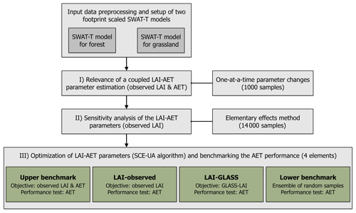
Figure 1 Methods applied in the present study to assess the significance of the LAI for AET estimation. Three different PET methods (Hargreaves, Priestley–Taylor, and Penman–Monteith) available in SWAT-T are applied for all three steps in the methodology.

2.1 Model description and parameter selection

The SWAT-T model is an enhanced version of the SWAT ecohydrological model (Arnold et al., 1998). In SWAT-T, the plant growth module has been modified to account for more realistic perennial plant phenology in tropical regions (Alemayehu et al., 2017), which can improve AET prediction (Zhang et al., 2020; Fernandez-Palomino et al., 2021; do Nascimento Ferreira, 2021; López-Ramírez et al., 2021). Apart from the plant growth module, SWAT-T and SWAT are identical. The original SWAT model has been applied worldwide in different river basins (Arnold and Fohrer, 2005; Tan et al., 2020) as well as regionally in Benin (Akoko et al., 2021). Specifically, most of the applications in Benin focused on discharge assessment for the Ouémé River basin (Bossa et al., 2014; Poméon et al., 2018) and its tributaries (Giertz et al., 2006; Bossa et al., 2012; Duku et al., 2016, 2018; Danvi et al., 2017; Togbévi et al., 2020). In previous studies in West Africa, remotely sensed AET was also used as a main calibration objective to predict streamflow (Odusanya et al., 2019, 2021). To the best of our knowledge, the SWAT-T model has not been applied in Benin, although it has been implemented in East Africa (Alemayehu et al., 2017).

Table 1 Approaches to compute potential evapotranspiration (E₀) and potential transpiration (T_plant) provided in SWAT-T.

The SWAT/SWAT-T model is generally spatially discretized into subbasins and subdivided into hydrological response units (HRUs). Three options are available to compute the potential ET (PET) in SWAT/SWAT-T: the temperature-based Hargreaves (PET-HG) method (Hargreaves and Samani, 1985), the energy-based Priestley–Taylor (PET-PT) method (Priestley and Taylor, 1972), and the combined temperature- and energy-based Penman–Monteith (PET-PM) method (Monteith, 1965). Table 1 summarizes the equations for PET (E₀) computation and highlights the integral part of the LAI in each approach.

In the equations in Table 1, λ is the latent heat of vaporization; H₀ is the extraterrestrial radiation; T_mx, T_mn, and T_av are the maximal, minimal, and mean daily temperature, respectively; α_pet is a coefficient; Δ is the slope of the saturation vapor pressure–temperature curve; γ is the psychrometric constant; H_net is the net radiation; G is the heat flux density to the ground; ρ_air is the air density; c_p is the specific heat at constant pressure; $e_{\mathrm{z}}^{\mathrm{0}}$ is the saturation vapor pressure of air at height z; e_z is the water vapor pressure of air at height z; r_a is the aerodynamic resistance; and r_c is the plant canopy resistance. In PET-PM, r_a and r_c are attributed to an alfalfa crop reference for the computation of E₀ (Neitsch et al., 2011). After the calculation of E₀, it is partitioned into potential plant transpiration (T_plant) and soil evaporation (E_soil). T_plant is computed depending on the values of the LAI for the given day for all PET methods. For PET-HG and PET-PT, a threshold of LAI =3.0 determines if T_plant is equal to E₀, i.e., all potential evapotranspiration is coming only from the plant transpiration without consideration of soil evaporation. If LAI ≤3.0, a share of E₀ is potentially available for T_plant and E_soil. For PET-PM, T_plant is computed using the Penman–Monteith equation (Table 1), in which r_a and r_c are determined using the modeled plant canopy and LAI. E_soil for the PET-PM model is then $E_{\text{soil}}=E_{\mathrm{0}}-T_{\text{plant}}$. The actual plant transpiration and soil evaporation are computed depending on the water availability and different biophysical parameters, such as the LAI or root depth, and soil properties, such as the field capacity. Actual plant transpiration and soil evaporation are then summed to the actual ET (AET).

The plant growth computation in SWAT/SWAT-T follows the approach of the Environmental Policy Impact Climate (EPIC) model (Arnold et al., 1998), in which the LAI is a key vegetation attribute for the plant phenology (Neitsch et al., 2011). Generally, the plant growth in SWAT/SWAT-T can be divided into an initial phase (start of the growing phase), a growing phase, a period of maturity (growing is halted to a constant LAI), a leaf senescence phase (natural decline in the plant and a decreasing LAI), and a dormancy period (no plant growth but a constant LAI). In the growing phase, the optimal leaf development in SWAT/SWAT-T is computed as follows:

$$\begin{array}{}\text{(1)}& {\mathrm{fr}}_{{\mathrm{LAI}}_{\text{mx}}}={\displaystyle \frac{{\mathrm{fr}}_{\text{PHU}}}{{\mathrm{fr}}_{\text{PHU}}+\exp (l_{\mathrm{1}}-l_{\mathrm{2}}\cdot {\mathrm{fr}}_{\text{PHU}})}},\end{array}$$

where ${\mathrm{fr}}_{{\mathrm{LAI}}_{\text{mx}}}$ is the fraction of the maximum leaf area index of a plant with respect to the fraction of the potential heat units for the plant, fr_PHU is the fraction of the potential heat units in the current day of the growth cycle, and l₁ and l₂ are shape coefficients. The plant growth continues until the maximum leaf area index is reached:

$$\begin{array}{}\text{(2)}& \begin{array}{rl}\mathrm{\Delta }{\mathrm{LAI}}_i=& ({\mathrm{fr}}_{{\mathrm{LAI}}_{\text{mx}},i}-{\mathrm{fr}}_{{\mathrm{LAI}}_{\text{mx}},i-\mathrm{1}})\cdot {\mathrm{LAI}}_{\text{mx}}\\ & \cdot (\mathrm{1}-\exp (\mathrm{5}\cdot ({\mathrm{LAI}}_{i-\mathrm{1}}-{\mathrm{LAI}}_{\text{mx}})\left)\right).\end{array}\end{array}$$

For perennial plants, the LAI for a given day i under optimal conditions is computed as follows:

$$\begin{array}{}\text{(3)}& {\mathrm{LAI}}_i={\mathrm{LAI}}_{i-\mathrm{1}}+\mathrm{\Delta }{\mathrm{LAI}}_i.\end{array}$$

However, the optimal plant growth can be constrained in SWAT/SWAT-T due to water, temperature, nitrogen, or phosphorous stress. The water stress (wstrs) is thereby directly linked to the actual plant transpiration and the total water plant uptake. The temperature stress (tstrs) is computed based on the air temperature of the given day and the user-defined parameters T_base and T_opt. Nitrogen and phosphorus stress (nstrs and pstrs, respectively) values are computed to account for insufficient nutrients (see Appendix for the additional equations). The actual plant growth is determined with a plant growth factor γ_reg:

$$\begin{array}{}\text{(4)}& {\mathit{\gamma }}_{\text{reg}}=\mathrm{1}-max(\mathrm{wstrs},\mathrm{tstrs},\mathrm{nstrs},\mathrm{pstrs}).\end{array}$$

The actual leaf area added on a day i is computed as follows:

$$\begin{array}{}\text{(5)}& \mathrm{\Delta }{\mathrm{LAI}}_{\text{act},i}=\mathrm{\Delta }{\mathrm{LAI}}_i\cdot {\mathit{\gamma }}_{\text{reg}}.\end{array}$$

The major difference between the plant growth modeling in SWAT and SWAT-T comprises two features: the logarithmic decline in the LAI and the automatic start of the growing phase based on a soil moisture index. In the first plant growth modification of SWAT, Strauch and Volk (2013) introduced a logarithmic decline in the LAI in the leaf senescence phase for a more realistic representation of the LAI decrease and to avoid a rapid drop in the LAI:

$$\begin{array}{}\text{(6)}& \mathrm{LAI}={\displaystyle \frac{{\mathrm{LAI}}_{\text{max}}-{\mathrm{LAI}}_{\text{min}}}{\mathrm{1}+\exp (-t)}},\end{array}$$

where t is defined considering the fraction of the potential heat units at which senescence become the dominant growth phase (${\mathrm{fr}}_{{\text{PHU}}_{\text{sen}}}$), as follows:

$$\begin{array}{}\text{(7)}& t=\mathrm{12}\cdot \left({\displaystyle \frac{\mathrm{1}-{\mathrm{fr}}_{\text{PHU}}}{\mathrm{1}-{\mathrm{fr}}_{{\text{PHU}}_{\text{sen}}}}}-\mathrm{0.5}\right)\text{if }{\mathrm{fr}}_{\text{PHU}}\ge {\mathrm{fr}}_{{\text{PHU}}_{\text{sen}}}.\end{array}$$

As plant growth in the tropics is generally governed by the water availability in the soils (Jolly and Running, 2004), Alemayehu et al. (2017) further modified the SWAT version of Strauch and Volk (2013) and implemented an automatic start of the growing phase that is triggered by the soil moisture index. For this purpose, the soil moisture index $\mathrm{SMI}=P/E_{\mathrm{0}}$ is introduced. The precipitation (P) is aggregated for a user-defined time window (here 5 d). An SMI threshold to start the growing has to be defined (here SMI=0.5). To avoid false starts of the new growing cycle, the end of the dry season (SOS₁, here October) and the beginning of the rainy season (SOS₂, here January) also have to be specified by the user (Alemayehu et al., 2017). In SWAT, the start of the growing phase is linked to the number of accumulated heat units. In SWAT-T, the soil moisture index has replaced this dependency on the heat units. The heat units are mainly used in SWAT-T to define the plant growth development over the year (see Eq. 1).

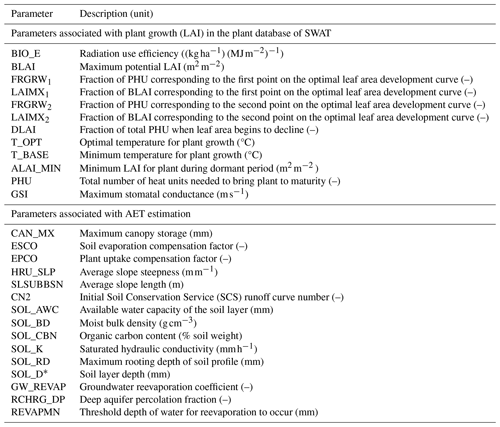
A total of 27 parameters have been selected to investigate the LAI–AET interaction (Table 2). The selection of LAI parameters follows the suggestion of Alemayehu et al. (2017), whereas the AET parameters are chosen based on a literature review. In the past, 27 SWAT parameters have been assessed for sensitivity analysis with a particular focus on AET (Ha et al., 2018; Odusanya et al., 2019; Bennour et al., 2022; Koltsida and Kallioras, 2022). Parameters with a coinciding low sensitivity reported in these studies, e.g., the hydraulic conductivity in the channel (CH_K2) or groundwater baseflow delay (GW_DELAY), are not considered in the present LAI–AET parameter list to reduce the total parameter space. For the present study, the soil layer thickness (SOL_D) is given for four soil layers from field measurements (Judex and Thamm, 2008). We adjust only the depth of the lowest soil layer in order to not excessively shape the ground-truth observations but to still facilitate an evaluation of the influence of the total soil thickness on the LAI–AET interaction in SWAT-T.

Table 2 List and description of parameters used to estimate the LAI and AET.

^∗ The lowest soil layer depth.

2.2 Study site and footprint-scale models

The study sites of Bellefoungou and Naholou are located in the western part of the Bétérou Catchment (Fig. 2). The climate is typical of sub-Saharan, subhumid Africa. The annual precipitation ranges from 1100 to 1500 mm (Mamadou et al., 2016; Bliefernicht et al., 2019). The precipitation pattern is unimodal, with the rainy season between April and October and the dry season from November to March. The annual mean daily temperature is 25 °C (Galle et al., 2018). The soils in the Bétérou Catchment consist of ferric soils with loamy sand present in the upper soil horizons (Giertz and Diekkrüger, 2003). Generally, the AET data follow the seasonality in the LAI (Fig. 2). However, a decrease in AET in the wet season can be observed in this region. AET depends on radiation, wind speed, and humidity. The net radiation decreases during the wet season, automatically reducing fluxes like sensible and latent heat (see Fig. A1). Additionally, the atmospheric demand is reduced because of high air humidity, which has been observed for the vapor pressure deficit (Mamadou et al., 2016), resulting in lower AET rates in the wet season.

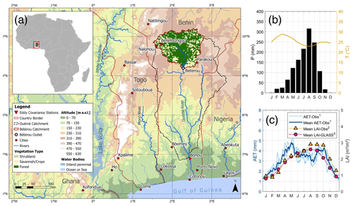
Figure 2 (a) Overview of the Bétérou Catchment and the locations of the eddy-covariance systems (Naholou and Bellefoungou); (b) the seasonality in precipitation and temperature in Bellefoungou; (c) and the comparison of observed AET (in blue), mean monthly values of the observed LAI (yellow), and mean monthly values of the GLASS LAI (in purple) in Bellefoungou. The solar radiation, wind speed, and relative humidity for the sites are illustrated in the Appendix (see Fig. A1). References for the data used to display the map are also listed in the Appendix (see Table A5). The superscripts in panel (c) denote the corresponding time periods: ¹ from January 2008 to December 2010; ² from July 2008 to May 2010; ³ from January 2007 to December 2015. Publisher's remark: please note that the above figure contains disputed territories.

The forested Bellefoungou region (9.791° N, 1.718°  E; 445 $\mathrm{m}\mathrm{a}.\mathrm{s}.\mathrm{l}.$) is covered with widespread woodland (clear forest) typical of sub-Saharan Africa (Ago et al., 2016). The Naholou region (9.74° N, 1.60°  E; 449 $\mathrm{m}\mathrm{a}.\mathrm{s}.\mathrm{l}.$) is covered mainly by a characteristic mixture of crops and savannah grassland and fallows (Ago et al., 2014). Due to the high share of grassland, the Naholou region is defined as a grassland region in the following. The estimated flux footprint extent for the grassland region is 4000 m², whereas this value is seasonally varying for the forested region and can be up to 60 000 m² (Mamadou et al., 2014). AET accounts for high shares of precipitation at both sites: the share of annual AET to precipitation is 57 % and 72 % for Naholou and Bellefoungou, respectively (Mamadou et al., 2016). The evaporative fraction (share of plant transpiration to total AET) is exceptionally high in the wet season. The values for the evaporative fraction are 70 ± 2.5 % at Naholou and 75 ± 0.7 % at Bellefoungou (Mamadou et al., 2016). These high plant transpiration rates to AET demonstrate the strong dependency of plant growth on AET in these regions (Mamadou et al., 2016; Hector et al., 2018). The field measurements of the LAI at both sites were delineated from hemispherical photographs and the processing methodology proposed by Weiss et al. (2004). The in situ data are complemented with corrections of an ensemble of satellite-based LAI products (CYCLOPE, MODIS, and SEVIRI) (Mamadou et al., 2014).

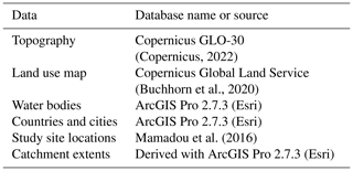
One SWAT-T model is set up for the forested and the grassland site in the Bétérou Catchment, respectively. Neither footprint calculations for the sites nor the necessary data to compute those are available. Thus, we adhere to the suggestion of Chu et al. (2021), who stated that radii of < 250 m around flux towers assure flux representativeness. The SWAT/SWAT-T models are watershed models. For the model delineation with SWAT-T, we drew circles (of 250 m radius) around each flux tower to guarantee the representativeness of the flux footprints. Based on the underlying digital elevation model (DEM), the resulting watershed extents are 8500 and 2300 m² for the forested and grassland sites, respectively. Although the footprint extent in the forested region can be larger depending on the season (Mamadou et al., 2016), we applied a constant extent following the suggestion of Chu et al. (2021). To ensure the homogeneity of land cover and soil properties, each SWAT-T model consists of a single HRU. The LAI and AET are simulated at a daily time step. The data sets used in this study are listed in Table 3. The land cover type for each site (forest or grassland) represented in the model is provided in Ago et al. (2014, 2016). We assigned the land use classes “FRSD” and “RNGE” from the SWAT crop database to the forested and grassland region, respectively. The observed AET data for both sites are available from 1 January 2008 to 31 December 2010 (Mamadou et al., 2016). The observed LAI data are available from 1 July 2008 to 31 May 2010 for the forested region (Bellefoungou; Ago et al., 2016) and from 5 August 2007 to 2 January 2010 for the grassland region (Naholou; Ago et al., 2014). The meteorological data provided by the AMMA-CATCH network date from 2005 to 2020 (Galle et al., 2018). The GLASS LAI data are provided from 2000 to 2021 (Liang et al., 2021). To enable the best possible overlap of measured LAI and AET data, the study periods from 1 January 2008 to 31 December 2010 and from 1 January 2007 to 31 December 2010 in the forested and grassland regions are defined, respectively.

(Copernicus, 2022)(Judex and Thamm, 2008)Mamadou et al. (2016)Ago et al. (2014)Mamadou et al. (2016)(Liang et al., 2021)(Galle et al., 2018)(Galle et al., 2018)(Galle et al., 2018)(Galle et al., 2018)(Galle et al., 2018)

Table 3 Overview of the data sets that are applied in this study.

2.3 Evaluation of the coupled LAI–AET parameter estimation

We postulate that the LAI and AET model parameters are decisive for a comprehensive plant growth modeling in SWAT-T, particularly if the accurate estimation of plant transpiration is a modeling objective. We apply parameter changes and compare the corresponding model responses to observed AET and LAI to assess the relevance of a coupled LAI–AET parameter estimation. Each parameter from Table 2 is randomly sampled (1000 samples), and the model is run for each sample. In each simulation, the other model parameters remain unaltered (one-at-a-time parameter changes). To avoid influences from poorly estimated parameter values (e.g., the default settings), the optimized model parameters from the LAI–AET optimization (see Sect. 2.5) are prescribed for the unaltered parameters. The model response to a parameter change is evaluated in two ways: with respect to observed AET and with respect to the observed LAI. Finally, an evaluation of how the LAI parameters influence the AET responses and how AET parameters influence the LAI responses is presented with this approach. The analysis of the LAI–AET parameter estimation is conducted for three PET methods (Hargreaves, Penman–Monteith, and Priestley–Taylor) for the forested study site. The results for the grassland region are similar but not explicitly presented.

2.4 Sensitivity analysis with the Morris method

A sensitivity analysis for all LAI–AET parameters is conducted to address the parameter response complexity of the coupled LAI–AET modeling with SWAT-T. Sensitivity analysis is an essential yet challenging step in the application of hydrological models and the evaluation of reliable parameter sets, particularly with respect to model equifinality. Different approaches exist to quantify the model responses to parameter changes. In this study, we take advantage of the elementary effects (or Morris) method (Morris, 1991), as its computational demand is inexpensive, the parameter sensitivity is statistically quantified, and nonlinear model responses can be determined (Morris, 1991; Campolongo et al., 2007). Moreover, parameters involved in parameter interactions and non-influential parameters can be identified.

Generally, the Morris method screens through a total sample size N, where one parameter, or input factor $q=[q_i,\mathrm{\dots },q_k]$, is changed while the others remain constant (one-at-a-time method). The total sample size N is generated based on r defined levels and q selected parameters such that $N=r(q+\mathrm{1})$. Based on each sample, the elementary effects d_i are calculated as follows:

$$\begin{array}{}\text{(8)}& \begin{array}{rl}{d}_i\left(q\right)& ={\displaystyle \frac{f(q_i,\mathrm{\dots },q_{i-\mathrm{1}},q_i+\mathrm{\Delta },q_{i+\mathrm{1}},\mathrm{\dots },q_k)-f\left(q\right)}{\mathrm{\Delta }}}\\ & ={\displaystyle \frac{f(q+\mathrm{\Delta }{e}_i)-f\left(q\right)}{\mathrm{\Delta }}},\end{array}\end{array}$$

where Δ represents the parameter step size, q+Δe_i denotes the transformed parameter point, $q=[q_i,\mathrm{\dots },q_k]$ is any selected parameter of N, and e_i consists of a vector of 0 values with a single value of 1 in the ith element. The index i refers to the current sample of N. The local sensitivity of parameter q is described with the value of d_i(q). For the global sensitivity, the statistical moments μ_i and σ_i, representing the mean and standard deviation from the distribution of the total sample simulation, are used (Morris, 1991). We use the absolute mean μ^∗, as proposed by Campolongo et al. (2007), so as to not disregard non-monotonic model responses because of opposite signs. The statistical moments for each set j are as follows:

$$\begin{array}{}\text{(9)}& {\displaystyle }& {\displaystyle }{\mathit{\mu }}_i^{\ast }\left(q\right)={\displaystyle \frac{\mathrm{1}}{r}}\sum _{i=\mathrm{1}}^r\left|d_i^j\left(q\right)\right|,\text{(10)}& {\displaystyle }& {\displaystyle }{\mathit{\sigma }}_i\left(q\right)=\sqrt{{\displaystyle \frac{\mathrm{1}}{r-\mathrm{1}}}\sum _{i=\mathrm{1}}^r{\left(d_i^j\left(q\right)-{\mathit{\mu }}_i\right)}^{\mathrm{2}}}.\end{array}$$

In this study, we quantify the model performance with the Kling–Gupta efficiency (KGE) (see Appendix for the additional equations). Moreover, we apply Latin hypercube sampling to guarantee a widespread input space. Using r=500 and q=27 parameters, the total sample size is N = 14 000. We investigated all 27 parameters in Table 2 for the sensitivity analysis. To apply the elementary effects method, we implemented the equations of Morris (1991) and Campolongo et al. (2007) into a set of MATLAB scripts.

2.5 Coupled LAI–AET parameter optimization and benchmarking

The LAI–AET parameters are first optimized with respect to different objectives: (i) a multi-objective optimization concerning LAI and AET (upper benchmark), (ii) an optimization only concerning observed LAI data (LAI-Obs), and (iii) an optimization only concerning satellite-based GLASS LAI data (LAI-GLASS). The model performance is then tested based on the benchmark proposed by Seibert et al. (2018), and the different objectives are compared. Seibert et al. (2018) have suggested using upper and lower model benchmarks to thoroughly evaluate the model performance of a specific modeling framework. In Seibert et al. (2018), the performance of the streamflow prediction is investigated. The application of a physically based model is thereby compared to an upper (optimized, conceptual model) and lower benchmark (ensemble of random samples) (Seibert et al., 2018). To avoid an arbitrary good or bad model response from a single parameter set, like the default model parameters, Seibert et al. (2018) propose using random parameter samples for the lower benchmark.

We apply the SCE-UA algorithm (Duan et al., 1994) to optimize the LAI–AET parameters. SCE-UA is a genetic algorithm by which samples of the parameters are stochastically generated first with respect to the lower and upper bounds of the parameter values. The parameter values are then changed to develop the samples to an optimum, i.e., to the optimal value of an objective function. We use the KGE to compare the simulated model output with the observed data. The algorithm application divides the initial sample into several subsamples (complexes) (Duan et al., 1994). In each complex, varying combinations of parameter values are embedded. Each complex is then used to produce offspring using the downhill simplex procedure (Nelder and Mead, 1965). The probability of a parameter value being used in the following complex is proportional to its model fitness, i.e., to the objective function. The new offspring replace parameter values of lower fitness. The main advantage of the SCE-UA algorithm is the application of (i) mutation, where new parameter values in the defined parameter spaces can be spontaneously generated, and (ii) shuffling, where recombination of the parameter values in new complexes is conducted (Duan et al., 1994).

Table 4 Summary of benchmark elements, their optimization approach with the corresponding optimization objectives, and their evaluation. For the lower benchmark, the median KGE of the AET performance of all 1000 random samples is used.

In this study, different objectives are defined for the LAI–AET parameter optimization (Table 4). First, the LAI–AET parameters are optimized in a multi-objective way with equal weight concerning observed AET and LAI (upper benchmark). This way, the performance potential of LAI–AET with respect to fitting both the AET and plant growth is quantified. Further, we also assess if detailed plant growth optimization can predict AET using the single LAI optimization approaches (LAI-Obs and LAI-GLASS). We use the SPOTPY toolbox (Houska et al., 2015) to apply the SCE-UA algorithm.

All three optimization approaches are compared based on the individual AET evaluation using the benchmarking proposed by Seibert et al. (2018). The upper benchmark is defined to be the best potential model performance (here upper benchmark in Table 4). We generated 1000 uniformly distributed LAI–AET parameter samples for the lower benchmark, evaluated the simulated AET with observed AET, and determined the overall median KGE performance as the lower benchmark. With the upper and lower model limits, the AET prediction performance of optimizing the parameters only for the LAI can be benchmarked for the footprint-scale models of the forested and grassland region as well as for different PET methods (PET-HG, PET-PT, and PET-PM). With 4 benchmark elements (Table 4), 2 land cover types, and 3 PET methods, 24 setups are compared to each other to assess the LAI–AET modeling performance of SWAT-T. In total, 27 parameters are considered for the sensitivity analysis. A total of 22 of the initially defined 27 parameters are optimized to reduce the parameter space and address the equifinality problem. Five parameters are not changed but are, rather, derived, e.g., from other regional studies. The groundwater parameters (GW_REVAP, RCHRG_DP, and REVAPMN) are obtained from Duku et al. (2015), who investigated streamflow prediction with SWAT for the Bétérou Catchment. The CN_2 numbers for FRSD and RNGE are derived from Alemayehu et al. (2017). The HRU_SLP and SLSUBBSN parameters are catchment-specific and individually derived when a SWAT/SWAT-T model is set up. Hence, we kept these geospatial parameters constant for optimization.

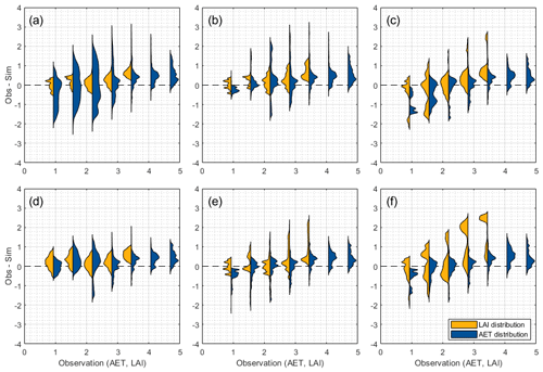
Figure 3 Distribution of variations in the AET or LAI for the one-at-a-time parameter changes (1000 samples) for the following parameters: (a) EPCO, (b) SOL_AWC, (c) PHU, (d) ALAI_MIN, (e) DLAI, and (f) T_BASE. The distributions are clustered in uniform intervals (size = 0.625) of the observed time series for the AET (mm) or LAI (m² m⁻²). The x axis indicates the observed AET (mm) and LAI (m² m⁻²) values. The y axis represents the difference between observed and simulated values with $\mathrm{\Delta }Y=\mathrm{Obs}-\mathrm{Sim}$ regarding AET (mm) or LAI (m² m⁻²). A perfect fit is indicated with the dashed line for ΔY=0. Positive and negative values show an underestimation and overestimation of the simulated values, respectively. The distributions (violin plots) are created based on Karvelis (2024).

3 Results

3.1 The relevance of a coupled LAI–AET parameter estimation

The influences of the parameter changes on both modeling objectives (LAI and AET) are displayed in Fig. 3. The evaluation shows the distribution of the results from each parameter change for AET and LAI. All 27 parameters for the PET methods used in this work impact the simulated LAI and AET. Figure 3 shows examples of the parameters (EPCO, SOL_AWC, PHU, ALAI_MIN, DLAI, and T_BASE) where the changes in both the LAI and AET are the most significant using the PET-PM model in the forested region. The results for PET-HG and PET-PT are illustrated in the Appendix.

As shown in Fig. 3, the variations in the parameter changes with respect to the intervals of the observed value are displayed. The AET and LAI data are clustered into seven and five intervals, respectively. We used the same interval size for the AET and LAI to improve readability. Each parameter change is then classified according to the interval. Next, the difference between observed and simulated data is calculated ($\mathrm{\Delta }Y=\mathrm{Obs}-\mathrm{Sim}$). The distributions are computed based on the difference within the interval. If, for example, the observed values for the AET interval of 0.625 to 1.25 mm are compared with the simulated values of the EPCO changes, an overall AET difference of −2.2 to 1.2 mm can be observed. The EPCO and SOL_AWC parameters are commonly associated with AET modeling. Thus, large spreads in the AET model response for the parameter changes can be observed, e.g., the influence of EPCO is exceptionally high for values of AET < 3 mm. However, the influence of both parameters on the LAI simulation is also indicated. For EPCO, decisive variations in the LAI response are observed for values of LAI > 2 m² m⁻². As plant growth is close to the phase of maturity, the significance of the plant water uptake in SWAT-T (determined with EPCO) increases, and the importance of EPCO for LAI modeling can be observed. Generally, the EPCO parameter governs the actual transpiration, which, in turn, influences the water stress of plants and, thus, affects the actual plant growth. The impact of EPCO on the LAI is significant, especially during the wet season when essential AET rates occur. With high AET, the plant growth stress is intensified in this period. Similarly, the available water capacity in the soil layers (SOL_AWC) influences the LAI response more the further the plant is into the growing phase (LAI > 2 m² m⁻²). The EPCO and SOL_AWC parameters can limit and influence plant growth in the wet season.

Concurrently, the shown LAI parameters (PHU, ALAI_MIN, DLAI, and T_BASE) influence both the AET and LAI. The variations in the simulated AET with respect to LAI parameter changes are particularly significant at the end of the wet season and during the dry season (AET < 3 mm). The PHU parameter determines when the plant reaches maturity based on the heat unit assumption. Similarly, the DLAI parameter defines when the LAI begins to decline and, thus, the start of leaf senescence. If the maturity phase is too early or short, the leaf senescence phase starts too early. In these cases, with respect to PHU and DLAI, the LAI–AET interaction is impaired, and influences on AET can be observed. The ALAI_MIN parameter defines the minimum LAI value for a plant type during the dormant period. If ALAI_MIN is set to an overly small value, the plant is underrepresented in the dry period, which results in low plant transpiration rates. The parameter changes for T_BASE result in the most extensive spread of simulated LAI values for all stages of the plant growth phase. With T_BASE, the temperature stress and the actual plant growth are determined in SWAT-T. The influence of the T_BASE parameter on AET is also present in the wet and dry periods of the AET modeling. Notably, the largest spreads of AET based on T_BASE can be observed for values of AET < 3 mm.

The one-at-a-time parameter change evaluation and the LAI–AET cross-comparison show that AET parameters, such as EPCO or SOL_AWC, are significant for AET and LAI modeling. Figure 3 also highlights that the LAI parameters, such as PHU, ALAI_MIN, DLAI, or T_BASE, can influence the AET model response. The variations in the LAI and AET resulting from changes in the remaining 21 LAI–AET parameters (see Table 2) are similar, although not shown here. Hence, a coupled LAI–AET parameter estimation is essential for the reliable computation of LAI and AET, particularly for perennial land cover types in a subhumid region in West Africa.

3.2 LAI–AET parameter sensitivity analysis concerning observed LAI

The sensitivities of the LAI–AET parameters are quantified using the elementary effects method regarding the observed LAI data. Figure 4 shows the statistical moments μ^∗ and σ for each parameter. It can be observed that nearly all parameters are located close to or slightly above the 1:1 line, which defines a nonlinearity of the parameters (Garcia Sanchez et al., 2014). Albeit with some exceptions, the parameters in the forested region result in higher σ values, implying that the parameter interactions are more nonlinear than in the grassland region. Generally, proximity of the parameter sensitivities for each land cover type method can be observed, e.g., the diamond symbols for the forest are close. Thus, differences between the PET methods and for the same land cover type are insignificant, suggesting potential independence of the LAI parameter sensitivity from the PET method. Moreover, all three groundwater parameters result in values μ^∗ = 0, thus denoting insensitivity to plant growth. Hence, they are excluded from the in-depth parameter analysis below.

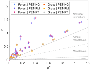
Figure 4 The statistical moments μ^∗ and σ of the elementary effects for the evaluation of the LAI–AET parameter sensitivity with respect to the observed LAI. We use the relation of $\mathit{\sigma }/{\mathit{\mu }}^{\ast }$ to classify regions of nonlinear, almost monotonous, monotonous, and linear parameter behavior (Garcia Sanchez et al., 2014).

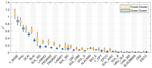
Figure 5 Clustering of the sensitivity analysis of all PET methods in the forest and grassland land cover types with respect to the observed LAI. The parameters are sorted according to the mean μ^∗ values resulting from the forested region. The superscript ¹ denotes that the parameter GSI is only accounted for when PET-PM is used.

Moreover, all PET methods are clustered to compare the sensitivity of the LAI–AET parameters for different land cover types. Figure 5 shows the distribution of μ^∗ when all PET methods are combined in one land cover group. The parameters are ranked according to the mean μ^∗ values from the simulations in the forested region. In Fig. 5, it can be observed that the general parameter sensitivity patterns are similar in the forested and grassland region, albeit with differences in the magnitude of μ^∗ for the land covers. The most sensitive parameters for both land use types are T_BASE, PHU, DLAI, BLAI, and SOL_RD. Moreover, a high box chart (high spread of μ^∗ values) implies high parameter interaction. The box plot heights for the forest and grassland clusters are generally comparable for the same parameters. If a parameter (e.g., T_BASE) in the forest region shows meaningful interactions, responses are also indicated for the same parameter in the grassland region alike. However, the BLAI and SOL_RD parameters appear to have higher parameter interactions in the forest than in the grassland region. Although the ranking is shown in Fig. 5 with respect to the mean μ^∗ values resulting from the forested region, the sensitivity hierarchy of the forested and grassland clusters is generally interchangeable.

From Fig. 5, a clear ranking pattern for PET methods and land use types can be observed (see also Fig. A4). Variations in the ranking position for each parameter are thereby minor, albeit with some exceptions for ALAI_MIN, GSI, EPCO, and ESCO. Earlier in the paper, in Fig. 3, the influence of EPCO on LAI was qualitatively illustrated. Here, the parameter sensitivity of EPCO to the LAI is quantified with μ^∗ and ranked with the other parameters in Fig. 5. The ranking differs for EPCO, GSI, and ESCO when PET-PM is used (Fig. A4). Its application implies that EPCO and ESCO are less relevant to the LAI model output, whereas GSI is more relevant. The stomatal conductance GSI is only accounted for in SWAT-T when PET-PM is used. Concurrently, the ALAI_MIN parameter is more highly ranked for grassland than for forest. Lower LAI values in the dry period of the rainy season increase the parameter ranking of ALAI_MIN. Ultimately, the plant growth parameters are generally more highly ranked than the AET parameters. Still, the rankings of SOL_RD, SOL_BD, SOL_CBN, SOL_D, and EPCO indicate an observable influence of AET parameters on the LAI. The sensitivity analysis of the LAI–AET parameters highlights that a coupled LAI–AET parameter estimation is inevitable for a comprehensive assessment of perennial plant growth of SWAT-T in subhumid regions for all three PET methods.

3.3 Optimization and benchmark testing of the LAI–AET modeling

The SCE-UA algorithm is applied to optimize the LAI–AET parameter in a multi-objective way (upper benchmark) and only concerning observed (LAI-Obs) or satellite-based (LAI-GLASS) LAI data. The evaluation focuses on observed AET in the following. The upper benchmark optimization results in very good modeling results for the three PET methods and two land cover types. For all six setups, the model performance (AET) of the upper benchmark results in values of KGE≥0.75 (Table 5). The performance of the LAI optimization to simulate AET results in values of KGE≥0.44 (LAI-Obs) and KGE≥0.49 (LAI-GLASS).

Table 5 Summary of final KGE values concerning observed AET and LAI for the benchmark elements. For the lower benchmark, the median AET performance of all 1000 random samples is determined. For LAI modeling, the LAI-GLASS optimization is investigated with the GLASS LAI. The lower benchmark LAI values are based on the parameterization of the median AET performance runs.

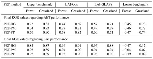
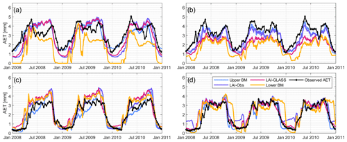
Figure 6 Time series of simulated and observed AET for the four benchmark elements with (a)  the PET-HG method in the forested region, (b) the PET-PM method in the forested region, (c) the PET-HG method in the grassland region, and (d) the PET-PM method in the grassland region.

The median of the random sampling (lower benchmark) determines values of KGE=0.45 to 0.74 across all six setups for AET. In the forested region, LAI-Obs and LAI-GLASS yield better predictions of AET than the lower benchmark, except for the PET-HG application and LAI-Obs optimization. However, this difference is negligible. Hence, a single optimization with LAI (observed or GLASS LAI) can improve the AET estimation in forested regions. The lower benchmark outperforms the LAI optimization (observed and GLASS LAI) in the grassland setups, although only with minor KGE differences. Considering that KGE≥0.5 is often accepted as a behavioral model performance (Rogelis et al., 2016; Knoben et al., 2019), the resulting KGE values for AET in the grassland setups are still satisfactory. Figure 6 shows the corresponding time series for AET. An overestimation of AET (PET-HG method), particularly in the wet period in the grassland region for the LAI optimization, can be observed. An underestimation of AET in the wet period is computed for the PET-PM method.

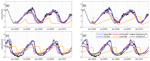
Figure 7 Time series of simulated, observed, and remotely sensed AET for the four benchmark elements with (a) the PET-HG method in the forested region, (b) the PET-PM method in the forested region, (c) the PET-HG method in the grassland region, and (d) the PET-PM method in the grassland region.

Generally, the best model performance is achieved by applying the PET-PM model, independent of the land cover type. The good AET fit for the LAI optimization approaches is explained by the LAI being a term used in calculating the canopy resistance in the PET-PM equation and the dynamic plant growth cycle. The LAI optimization guarantees a steady transpiration rate, even in the dry period, without the plant dying, i.e., LAI dropping to zero. The lower benchmark with no tailored LAI modeling outputs an underestimation of AET in the dry season (Fig. 6), which can be attributed to its low LAI values in this season (Fig. 7). The simulated LAI and AET data for PET-PT are similar to the PET-HG results (see Fig. A5). Concurrently, good model performance for PET-PM is also achieved for the lower benchmark. Although insufficient LAI modeling performance results for the lower benchmarks in the grassland region, acceptable AET performance is still achieved (Table 5). Ultimately, the results show that SWAT-T can make accurate LAI and AET predictions. Moreover, the benchmarking test shows that, even if no AET data are available, the LAI parameter optimization with observed or satellite-based LAI facilitates an acceptable AET estimation in forest and grassland regions. However, the AET performance resulting from LAI calibration is constrained by the hydrometeorological data availability for the choice of the PET method and whether the application of energy-based PET methods, particularly PET-PM, is feasible.

4 Discussion and outlook

4.1 Evaluation of the LAI–AET parameters with observed and GLASS LAI

This study evaluates LAI modeling with observed and satellite-based LAI data. Previous studies with SWAT have also employed field measurements for the LAI (Park et al., 2017; Yang et al., 2018; Nantasaksiri et al., 2021) or forest biomass production (Khanal and Parajuli, 2014; Haas et al., 2022) to evaluate the LAI modeling ability of SWAT. However, the parameters used in these studies differ, e.g., the total number of parameters applied ranges from 3 (Yang et al., 2018) to 18 (Haas et al., 2022). The suggested LAI parameter list for SWAT-T in Alemayehu et al. (2017) consists of 11 parameters. We applied one-at-a-time parameter changes to assess the interaction of LAI and AET parameters on both simulated LAI and AET data. We compared the resulting model responses (LAI and AET) for each parameter change and computed the influences of LAI parameters on AET modeling and vice versa. Although the assessment of the one-at-a-time changes was based on a qualitative analysis, a clear pattern of the reciprocal influences became apparent. Hence, we extended the LAI parameter list and identified 27 LAI–AET parameters for the evaluation of the significance of the LAI for AET estimation in SWAT-T.

We applied the elementary effects method to evaluate the parameter sensitivity in order to understand the parameter interactions in SWAT-T with observed LAI data. Previous efforts to assess the sensitivity of LAI parameters have focused on a relative sensitivity index (Khanal and Parajuli, 2014; Nantasaksiri et al., 2021). In the present study, for the first time, the sensitivity of the comprehensive set of 27 LAI–AET parameters is quantified with the elementary effects method in SWAT-T. Previously, the Morris screening method has been used for the sensitivity analysis of SWAT model parameters only concerning discharge (Xiang et al., 2022; Abbas et al., 2024). With the application of the Morris screening, a ranking of the sensitivity of the parameters is determined in the present study. The most influential parameters with respect to the LAI are T_BASE, PHU, DLAI, and BLAI, independent of the land cover type or the PET method. Moreover, SOL_RD is the parameter with the highest influence on the other parameters. Its influence is significant because it defines the root depth within the soils, which in turn determines the plant water uptake and, thus, the growing efficiency. The impact of SOL_RD is significant in the forested region, where the uptake of plants is high and roots grow deep. The sensitivities reported in Khanal and Parajuli (2014) are highest for the DLAI, BIO_E, BLAI, and SOL_RD parameters. Nantasaksiri et al. (2021) identified the BIO_E, HVSTI (defined as the potential harvest index for the plant at maturity given ideal growing conditions), BLAI, LAIMX₂, and DLAI parameters to be the most sensitive. The findings in both studies are coherent with our results, albeit with the missing investigation of some of the most sensitive parameters, e.g., T_BASE and PHU. Moreover, we apply a global sensitivity measure, whereas Khanal and Parajuli (2014) and Nantasaksiri et al. (2021) used a local measure (relative sensitivity index). However, local measures are limited if the model response is nonlinear (Saltelli et al., 2008), which is the case for the LAI–AET parameters concerning observed LAI (Fig. 4). Thus, we could detect and address the nonlinearity of the LAI–AET parameters with the elementary effects method in the present study.

The field measurements used in this study are derived from hemispherical photographs and satellite-based corrections. Such assorted LAI data can be subject to uncertainties (Fang et al., 2019). To address the potential shortcomings of LAI observations, we additionally evaluated the LAI estimation regarding satellite-based GLASS LAI. Thus, for both land cover types, the performance of the LAI prediction is accurate, independent of the PET method. We applied the GLASS LAI data, as they are reliable in different regions worldwide (Liang et al., 2014) and robust to the noise and uncertainties that satellite-based vegetation can be susceptible to in tropical regions (Viovy et al., 1992; Atkinson et al., 2012). The dual consideration of both observed and GLASS LAI data ensured the comprehensive LAI evaluation in the present study.

4.2 Optimization and benchmarking of the AET modeling with observed AET at the footprint scale

The model extent of the grassland region (2300 m²) represents the actual footprint size of 4000 m² estimated by Mamadou et al. (2014) well. The footprint for the forested region is seasonally varying and can be up to 60 000 m² (Mamadou et al., 2014). Generally, the source area of AET in EC systems can fluctuate over the year (Kim et al., 2018) due to, for example, the wind direction – the wind rose can influence the extent of the footprint (Chen et al., 2009; Chu et al., 2021). As the model extents of SWAT-T are constant for the modeling period and the necessary data were unavailable, we approximated the model scale to represent the footprint for the whole season according to Chu et al. (2021). The main objective of the present study is the thorough evaluation of the vertical fluxes (AET) based on the LAI–AET interaction in SWAT-T. In SWAT/SWAT-T, the vertical fluxes (AET) are computed at the HRU level. Hector et al. (2018) investigated the same regions using a physically based model for the critical zone (ParFlow-CLM) and also concluded that vegetation is a significant factor in the AET estimation, which is coherent with our findings.

In the present study, we also investigated whether detailed LAI modeling disregarding AET can predict reliable AET estimates in SWAT-T. We showed that LAI optimization also facilitates an adequate behavioral modeling of AET with acceptable KGE values for both land cover types. However, evaluating the model performance when only the values of one efficiency metric (e.g., KGE) are considered can be misleading, as the explanatory power of the model is missing (Schaefli and Gupta, 2007; Knoben et al., 2019). Information on whether a modeling approach is applicable or should be rejected and the assessment of the strengths and deficiencies of the modeling approach need to be covered using the pure values of one efficiency metric (e.g., KGE) (Knoben et al., 2019). To address these shortcomings of an exclusive KGE value evaluation, we applied the benchmarking test proposed by Seibert et al. (2018). The comparison of modeling approaches, such as the single LAI optimization with upper and lower benchmark levels, facilitated the assessment of whether detailed LAI modeling (single LAI optimization) can improve the LAI prediction in SWAT-T. The benchmarking showed that the significance of thorough LAI modeling is more pronounced in the forested than in the grassland region.

4.3 Impacts of the model structure on the AET estimation

At a daily time step, the temporal dynamics of simulated AET fit adequately to the observed AET pattern in the dry and wet season for all three PET methods. Thus, the application of PET-PM outperforms PET-HG and PET-PT. Generally, the PET-PM application is more physically complex than PET-HG and PET-PT but requires more input data. The computation of PET-HG and PET-PT relies on empirically delineated coefficients, e.g., H₀ and α_pet, respectively. In PET-PM, terms for different properties of the land–atmosphere interaction are implemented, such as vapor pressure or the canopy resistance (r_c) and aerodynamic resistance (r_a). In PET-PT, however, the aerodynamic term α_pet is modeled with a constant coefficient of 1.28 (Neitsch et al., 2011). Moreover, the partitioning of PET into potential plant transpiration and soil evaporation is based on a threshold in PET-HG and PET-PT. While PET-PM estimates the potential transpiration using the Penman–Monteith equation, in which r_c and r_a are dependent on the LAI modeling, the partitioning of PET implemented in PET-PT and PET-HG is based on the threshold LAI>3.0. Hence, the significance of detailed LAI modeling in these methods has less impact on plant transpiration. For the forested region, the LAI modeling (single LAI optimization disregarding AET) can still predict the AET adequately. The influence of the LAI estimation is less substantial in the grassland region, where the lower benchmark (random sampling) outperforms the single LAI optimization (observed and GLASS LAI). However, the physical representation of the LAI–AET relationship is limited, as low KGE values are computed. Overall, the more straightforward approaches PET-HG and PET-PT can still yield adequate AET outputs (Archibald and Walter, 2014), although PET-PM offers a more physically sound depiction of the LAI–AET interaction.

In previous studies, similarly accurate AET performance for the PET-PM application has been observed for a forested region (do Nascimento Ferreira, 2021) and for a grassland region (Qiao et al., 2022) regarding a comparison with AET from EC systems. An improvement in the AET estimation with SWAT-T using EC systems was been demonstrated for PET-HG, PET-PT, and PET-PM at the HRU scale in López-Ramírez et al. (2021), where the annual budgets for AET were found to fit best for PET-HG. However, no coupled LAI–AET parameterization has been considered. We were able to address the relevance of the coupled LAI–AET parameterization and, thereby, also demonstrate the best overall performance for PET-PM.

4.4 Outlook

The elementary effects were computed based on the period for which measured LAI data are available. SWAT-T divides plant growth into four phases (start of growth, maturity, leaf senescence, and dormancy). A time-varying sensitivity analysis of the LAI–AET parameters with respect to the plant growth phases should be done in future work. Applications should explore approaches such as dynamic identifiability analysis (Wagener et al., 2003) or wavelet-based methods (Chiogna et al., 2024). These time-varying approaches can further improve our understanding of the LAI–AET parameter interaction.

We showed that the LAI–AET modeling of SWAT-T for approximated footprints is applicable for perennially vegetated regions in West Africa. In future work, coupled LAI–AET modeling should be transferred from the footprint to the catchment scale. The water balance of the ecosystems of West Africa is mainly characterized by a high share of AET. Hence, this study focuses on analyzing the LAI–AET interaction and, thus, on the dominant vertical fluxes in these regions. Given the significance of AET in West Africa, the LAI–AET relationship can also be essential for estimating the horizontal fluxes that are substantial for streamflow computation at the catchment scale. Applying satellite-based LAI data, e.g., GLASS LAI, can also support plant growth and AET modeling at larger scales. Moreover, we focused our analysis on characteristic regions of West Africa. Future work should analyze the LAI–AET interaction for other land cover types, e.g., regions with higher LAI values like the Congo forests or other climatic zones, such as energy-limited regions.

The present study focuses on the LAI as a vegetation attribute. In SWAT/SWAT-T, the canopy height is also modeled. The canopy height can impact the PET estimation, e.g., in the application of PET-PM, where the canopy resistance (r_c) is a function of the canopy height. Moreover, EC systems can also offer other relevant attributes of the vegetation–AET interaction, such as derivations of the aerodynamic conductance, surface conductance, water vapor, heat fluxes, or the evaporative fraction (Mamadou et al., 2016). These attributes improve the physical understanding of the vegetation–AET interaction and can also be valuable to inform hydrological modeling (Hector et al., 2018). We focused on the application of the LAI because (i) it is a key vegetation attribute in SWAT-T and (ii) global products of LAI are available. As the seasonal dynamics of both forest and grassland vegetation (LAI) are modeled accurately, we postulate that the approaches of this study can be transferred to other plant and crop types.

Considering a coupled LAI–AET parameterization, the quantification of biomass or crop yield for other plant species can also be addressed. Yang and Zhang (2016) investigated the biomass as a proxy for primary productivity with SWAT for different flux sites of the AmeriFlux network. They identified BIO_E, BLAI, T_OPT, T_BASE, and BIO_LEAF as the most significant parameters for biomass. Apart from the BIO_LEAF parameter, the choice of parameters is similar to our study. Hence, LAI modeling can also be used as a proxy for biomass estimation. However, in-depth analysis with observed biomass data is inevitable if the modeling objective is the evaluation of biomass and net primary productivity.

5 Conclusion

The broad implication of this research is the presentation of a comprehensive LAI–AET parameter evaluation to model both the LAI and AET using an ecohydrological model. We highlighted the relevance of a coupled LAI–AET parameter estimation in SWAT-T. Although the impact of LAI parameters on the AET prediction can be low, substantial influence can be observed on the AET dynamics. The impact of the LAI parameters on AET is exceptionally high at the end of the wet season and the beginning of the dry season, when the plant growth phase shifts from plant maturity to leaf senescence. Moreover, the affect of water stress on plant growth resulting from the AET estimation can be decisive and should be considered for comprehensive LAI modeling. We conclude that the relevance of a coupled LAI–AET parameter estimation indicates that a stepwise modeling approach (e.g., first LAI and then AET) requires a careful review of the simulated LAI after the AET parameters are estimated. An analysis using the elementary effects method demonstrates that most LAI parameters behave nonlinearly if compared with observed LAI data. The most sensitive parameters for LAI modeling are those associated with LAI parameters. However, a Morris screening also indicates a meaningful contribution from the soil parameters. The ranking further illustrates the independence of the LAI parameters with respect to the land cover type (forest and grassland).

The multi-objective optimization with the SCE-UA algorithm results in accurate estimations of both the LAI and AET for all PET-methods and land cover types. SWAT-T has also been proven to be applicable at the footprint scale in West Africa. Although the simpler PET-HG and PET-PT methods facilitate satisfactory modeling results, applying the PET-PM method outperforms these methods for the LAI and AET estimation in the forested and grassland regions. Moreover, our work demonstrates that an adequate estimation of AET can be obtained if the LAI–AET parameters are only optimized with respect to LAI data (and disregarding AET data) for forest and grassland regions. Compared with the lower benchmark level, the benchmark test illustrates an enhancement of the AET prediction for the PET methods (particularly PET-PT and PET-PM). This is particularly noteworthy for data-scarce regions where no field measurements of AET are available. Even if no observed LAI data for a forested region are available, practitioners and researchers can optimize the LAI–AET parameters using remotely sensed LAI data and still achieve reliable AET estimations. In the grassland region, the resulting AET prediction from the LAI optimization is also adequate. However, the lower benchmark indicates better performance for the grassland site. The good result of the lower benchmark is obtained from the median KGE performance of a large number of parameter samples (1000 runs). Single parameter changes, the mean, or the default model parameter values of the SWAT/SWAT-T crop database do not necessarily facilitate satisfactory AET prediction. Overall, the LAI–AET parameter optimization for grassland yields sufficient AET performance. Nevertheless, its role in the AET estimation is less critical than for forested regions.

Finally, we stress the importance of opting for a coupled parameter estimation to understand the LAI–AET interaction and to improve the land–atmosphere simulation in hydrological modeling. The performance comparison of modeled AET confirms that a detailed plant growth analysis is essential. The highlighted relevance of the LAI–AET interaction is significant for a thorough quantification of hydrological processes and, hence, necessary for the comprehensive assessment of water resources management.

Appendix A

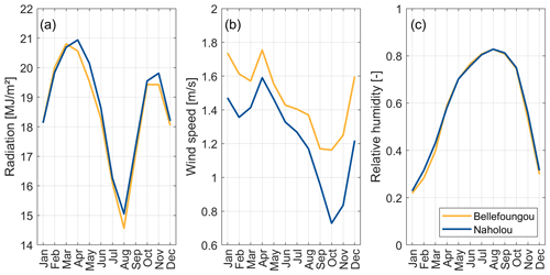
Figure A1 Seasonality in (a) daily total solar radiation, (b) wind speed, and (c) relative humidity for the Bellefoungou (forest) and Naholou (grass) study sites. The seasonality is derived from measurements of each eddy-covariance system.

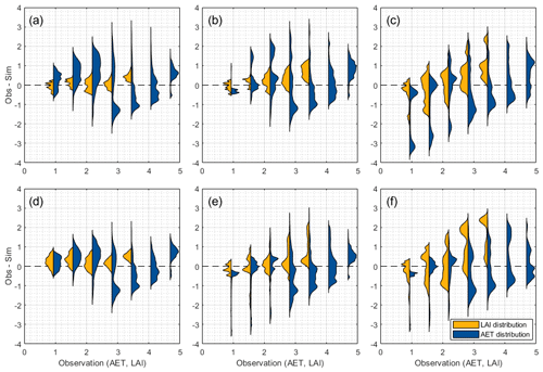
Figure A2 Distribution of variations in the AET or LAI for the one-at-a-time parameter changes for PET-HG for the following parameters: (a) EPCO, (b) SOL_AWC, (c) PHU, (d) ALAI_MIN, (e) DLAI, and (f) T_BASE. The distributions are clustered in uniform intervals (size = 0.625) of the observed time series for the AET (mm) or LAI (m² m⁻²). The x axis indicates the observed AET (mm) and LAI (m² m⁻²) values. The y axis represents the difference between observed and simulated values with $\mathrm{\Delta }Y=\mathrm{Obs}-\mathrm{Sim}$ regarding the AET (mm) or LAI (m² m⁻²). A perfect fit is indicated with the dashed line for ΔY=0. Positive and negative values show an underestimation and overestimation of the simulated values, respectively. The distributions (violin plots) are created based on Karvelis (2024).

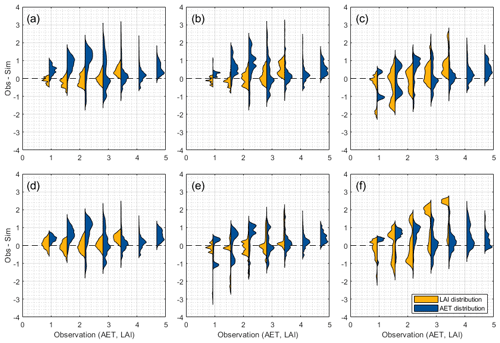
Figure A3 Distribution of variations in the AET or LAI for the one-at-a-time parameter changes for PET-PT for the following parameters: (a) EPCO, (b) SOL_AWC, (c) PHU, (d) ALAI_MIN, (e) DLAI, and (f) T_BASE. The distributions are clustered in uniform intervals (size = 0.625) of the observed time series for the AET (mm) or LAI (m² m⁻²). The x axis indicates the observed AET (mm) and LAI (m² m⁻²) values. The y axis represents the difference between observed and simulated values with $\mathrm{\Delta }Y=\mathrm{Obs}-\mathrm{Sim}$ regarding the AET (mm) or LAI (m² m⁻²). A perfect fit is indicated with the dashed line for ΔY=0. Positive and negative values show an underestimation and overestimation of the simulated values, respectively. The distributions (violin plots) are created based on Karvelis (2024).

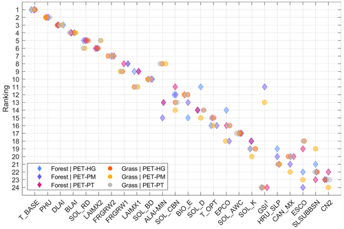
Figure A4 Ranking of the LAI–AET parameter sensitivity for the three PET methods and two land cover types with respect to the observed LAI. The superscript ¹ denotes that parameter GSI is only accounted for when PET-PM is used.

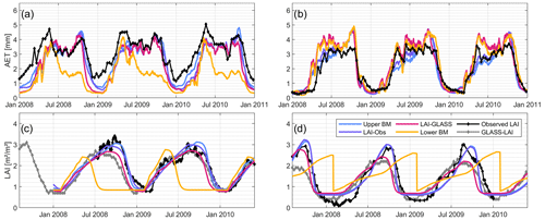
Figure A5 Time series of simulated and observed AET and LAI for the four benchmark elements computed with the PET-PT method with the following: (a) AET in the forested region, (b) AET in the grassland region, (c) LAI in the forested region, and (d) LAI in the grassland region.

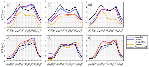
Figure A6 Seasonality in the simulated and observed AET time series. The top row (a–c) shows the AET data for the forested region for different PET methods, with applications of (a) PET-HG, (b) PET-PM, and (c) PET-PT. The bottom row (d–f) shows the grassland region, with applications of (d) PET-HG, (e) PET-PM, and (f) PET-PT.

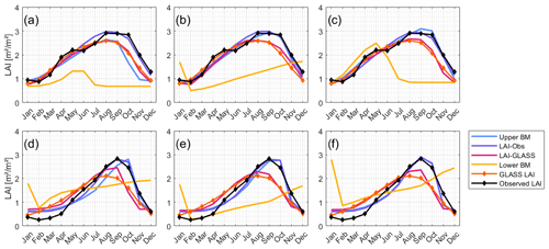
Figure A7 Seasonality in the simulated and observed LAI time series. The seasonality in LAI-Obs and GLASS LAI is displayed. The top row (a–c) shows the LAI data for the forested region for different PET-methods, with applications of (a) PET-HG, (b) PET-PM, and (c) PET-PT. The bottom row (d–f) shows the grassland region, with applications of (d) PET-HG, (e) PET-PM, and (f) PET-PT.

Water stress (wstrs) is calculated as follows:

$$\begin{array}{}\text{(A1)}& \mathrm{wstrs}=\mathrm{1}-{\displaystyle \frac{E_{\mathrm{t},\text{act}}}{E_{\mathrm{t}}}}=\mathrm{1}-{\displaystyle \frac{w_{\text{actualup}}}{E_{\mathrm{t}}}},\end{array}$$

where E_t,act is the actual transpiration, E_t is the potential plant transpiration, and w_actualup is the total water uptake. w_actualup is computed based on the amount of water in the soil layer and the water content at the wilting point (for details, refer to Neitsch et al., 2011).

Temperature stress (tstrs) is calculated as follows:

$$\begin{array}{}\text{(A2)}& \begin{array}{rl}& \mathrm{tstrs}=\\ & \left\{\begin{array}{ll}\mathrm{1},& \text{if }{T}_{\text{av}}\le T_{\text{base}}\\ \mathrm{1}-\exp \left(\frac{-\mathrm{0.1054}\cdot (T_{\text{opt}}-T_{\text{av}}{)}^{\mathrm{2}}}{(T_{\text{av}}-T_{\text{base}}{)}^{\mathrm{2}}}\right),& \text{if }{T}_{\text{base}}<T_{\text{av}}\le T_{\text{opt}}\\ \mathrm{1}-\exp \left(\frac{-\mathrm{0.1054}\cdot (T_{\text{opt}}-T_{\text{av}}{)}^{\mathrm{2}}}{(\mathrm{2}\cdot T_{\text{opt}}-T_{\text{av}}-T_{\text{base}}{)}^{\mathrm{2}}}\right),& \text{if }{T}_{\text{opt}}<T_{\text{av}}\le \mathrm{2}\cdot T_{\text{opt}}-T_{\text{base}}\\ \mathrm{1},& \text{if }{T}_{\text{av}}>\mathrm{2}\cdot T_{\text{opt}}-T_{\text{base}},\end{array}\right.\end{array}\end{array}$$

where T_av is the mean air temperature for the day, T_base is the base temperature of the plant for growth, and T_opt is the optimal temperature of the plant for growth.

Nitrogen stress (nstrs) is calculated as follows:

$$\begin{array}{}\text{(A3)}& \mathrm{nstrs}=\mathrm{1}-{\displaystyle \frac{{\mathit{\varphi }}_{\mathrm{n}}}{{\mathit{\varphi }}_{\mathrm{n}}+\exp (\mathrm{3.535}-\mathrm{0.02597}\cdot {\mathit{\varphi }}_{\mathrm{n}})}},\end{array}$$

where ϕ_n is a scaling factor for nitrogen stress computed with the actual and optimal mass of nitrogen stored in the plant material (bio_N and bio_N,opt, respectively):

$$\begin{array}{}\text{(A4)}& {\mathit{\varphi }}_{\mathrm{n}}=\mathrm{200}\cdot \left({\displaystyle \frac{{\mathrm{bio}}_{\mathrm{N}}}{{\mathrm{bio}}_{\mathrm{N},\text{opt}}}}-\mathrm{0.5}\right).\end{array}$$

Phosphorus stress (pstrs) is calculated as follows:

$$\begin{array}{}\text{(A5)}& \mathrm{pstrs}=\mathrm{1}-{\displaystyle \frac{{\mathit{\varphi }}_{\mathrm{p}}}{{\mathit{\varphi }}_{\mathrm{n}}+\exp (\mathrm{3.535}-\mathrm{0.02597}\cdot {\mathit{\varphi }}_{\mathrm{p}})}},\end{array}$$

where ϕ_p is a scaling factor for phosphorous stress computed with the actual and optimal mass of phosphorus stored in the plant material (bio_P and bio_P,opt, respectively):

$$\begin{array}{}\text{(A6)}& {\mathit{\varphi }}_{\mathrm{p}}=\mathrm{200}\cdot \left({\displaystyle \frac{{\mathrm{bio}}_{\mathrm{P}}}{{\mathrm{bio}}_{\mathrm{P},\text{opt}}}}-\mathrm{0.5}\right).\end{array}$$

The Kling–Gupta efficiency (KGE) is calculated as follows:

$$\begin{array}{}\text{(A7)}& \mathrm{KGE}=\mathrm{1}-\sqrt{(r-\mathrm{1}{)}^{\mathrm{2}}+{\left({\displaystyle \frac{{\mathit{\sigma }}_{\text{sim}}}{{\mathit{\sigma }}_{\text{obs}}}}-\mathrm{1}\right)}^{\mathrm{2}}+{\left({\displaystyle \frac{{\mathit{\mu }}_{\text{sim}}}{{\mathit{\mu }}_{\text{obs}}}}-\mathrm{1}\right)}^{\mathrm{2}}},\end{array}$$

where r is the linear correlation between observations and simulations; σ_sim and σ_obs are the standard deviation of the simulations and observations, respectively; and μ_sim and μ_obs are the mean value for the simulations and observation, respectively.

Table A1 List of final parameters for the multi-objective (LAI and AET), observed LAI, and GLASS LAI optimization for the forested region. The units of the parameters are excluded for readability; they are given in Table 2.

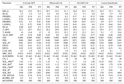
^a Lowest soil layer depth. ^b Relative parameter changes: para${}_{\text{new}}={\mathrm{para}}_{\text{original}}+{\mathrm{para}}_{\text{original}}\cdot {\mathrm{para}}_{\text{change}}$.

Table A2 List of final parameters for the multi-objective (LAI and AET), observed LAI, and LAI-GLASS optimization for the grassland region. The units of the parameters are excluded for readability; they are given in Table 2.

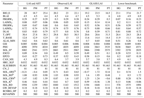
^a Lowest soil layer depth. ^b Relative parameter changes: para${}_{\text{new}}={\mathrm{para}}_{\text{original}}+{\mathrm{para}}_{\text{original}}\cdot {\mathrm{para}}_{\text{change}}$.

Table A3 Water balance components for the final runs for the forested region. All quantities listed are in millimeters. The components of the lower benchmark are shown, although no calibration was applied.

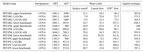
^∗ GW is short for groundwater.

Table A4 Water balance components for the final runs for the grassland region. All quantities listed are in millimeters. The components of the lower benchmark are shown, although no calibration was applied.

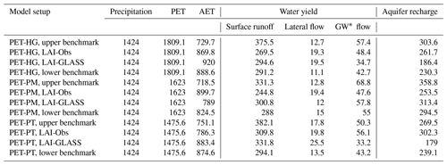
^∗ GW is short for groundwater.

(Copernicus, 2022)(Buchhorn et al., 2020)Mamadou et al. (2016)

Table A5 Overview of the data used for the study site map.