Phosphorus transport in a hotter and drier climate: in-channel release of legacy phosphorus during summer low-flow conditions

“Legacy phosphorus” is the historical accumulation of phosphorus (P) in soils and sediments due to past human inputs. River networks represent a potential sink and/or source of legacy P, with many in-channel processes potentially governing the storage and mobilization of P over time. The objective of this study was to evaluate the potential contribution of the in-channel release of legacy P to bioavailable P transport in streams during summer low-flow conditions across a land use gradient in Minnesota, USA. We addressed this objective through the synthesis of (1) water quality and streamflow (Q) data collected for 143 gauged watersheds across the state of Minnesota between 2007–2021 (22 750 total samples); (2) water quality data from 33 additional ditch, stream, and river sites in Minnesota sampled under low-flow conditions in the summer of 2014; and (3) water quality data collected from tile drainage outlets for 10 monitored farm fields between 2011–2021. We used geospatial data and a random forest modeling approach to identify possible drivers of bioavailable P concentrations during summer low flows for gauged watersheds. During low flows in late summer, between one-third to one-half of the gauged watersheds we studied exhibited soluble reactive phosphorus (SRP) concentrations that were above previously identified thresholds for eutrophication of 0.02–0.04 mg L⁻¹. For many of these watersheds, stream SRP concentrations in late summer were above those observed in tile drainage outlets. Elevated SRP concentrations during late-summer low flows weakened concentration–discharge relationships that would otherwise appear to indicate more strongly mobilizing SRP–Q responses across other seasons and flow conditions. While wastewater discharge likely contributed to elevated P concentrations for watersheds with high densities of treatment plants, many watersheds did not have substantial wastewater impacts. The most important variables for predicting bioavailable P concentrations during late-summer low-flow conditions in a random forest model were land use in riparian areas (particularly crop cover); soil characteristics including soil erodibility, soil permeability, and soil clay content; agricultural intensity (reflected via higher pesticide use, higher phosphorus uptake by crops, and higher fertilizer application rates); watershed precipitation; and stream temperature. These findings suggest that, for stream and river sites heavily impacted by past and current P inputs associated with agriculture and urbanization, biogeochemical processes mediated by climate and geology can result in the release of legacy P from in-channel stores during late-summer low-flow conditions. As summers become hotter and, at times, drier – which are predicted changes in this region – conditions for the release of legacy P stored in stream and river channels will likely become more prolonged and/or more acute, increasing eutrophication risk.

1 Introduction

Phosphorus (P) inputs arising from urbanization and industrial or intensive agriculture have resulted in widespread eutrophication of freshwater and marine environments. Excessive inputs of P along with nitrogen (N) have resulted in costly and sometimes dangerous conditions for human society, including increased prevalence of harmful algal blooms, contamination of drinking-water supplies, decreased recreational opportunities, loss of critical marine fisheries, and negative impacts on biodiversity (Bennett et al., 2001). This problem is particularly acute in the midwestern Corn Belt of the United States, which represents a global hotspot for P fertilization (Haque, 2021).

Most progress in the reduction of P release to the environment has come from the implementation of improved wastewater infrastructure (Keiser and Shapiro, 2019). However, diffuse (nonpoint) sources of P, such as those arising from agricultural and urban landscapes, have yet to be substantially curtailed and remain largely unregulated. In addition to ongoing P inputs to the environment, water quality is also impacted by the existing supply of “legacy P” in the landscape (Goyette et al., 2018). Legacy P is the historical accumulation of P in soils and sediments due to past land use practices, such as agricultural fertilization, the spreading of manure, and wastewater discharge.

Efforts are underway to understand sources of legacy P in the terrestrial environment, including agricultural soils and riparian buffers (e.g., Osterholz et al., 2020). Lentic waterbodies (lakes, impoundments, and wetlands) are well known for their potential to remobilize stored P and become sources instead of sinks for downstream P, especially at high rates of nutrient inputs (e.g., Vilmin et al., 2022). The river network itself represents another potential sink and/or source of legacy P, with many dynamic in-channel processes potentially governing the storage and mobilization of P over time. For example, benthic redox conditions, in-stream primary productivity, microbial respiration, and sediment adsorption–desorption can all modulate whether P is retained in stream sediments, temporarily immobilized as organic P, or released to the water column as bioavailable P (Records et al., 2016).

We previously observed that concentrations of bioavailable P (i.e., soluble reactive phosphorus, SRP) in agriculturally dominated streams and rivers of Minnesota were often elevated during low-flow conditions in late summer (Dolph et al., 2019). However, questions remained about whether the elevated SRP we observed in late summer was sourced predominantly from tile drainage (therefore being indicative of legacy and/or current P sources stored in farm soils), from point sources such as wastewater treatment plants, or possibly from legacy sources in the river network itself. Tile drainage is extensive across the agricultural Midwest (Valayamkunnath et al., 2020) and has been found to contribute substantially to and even dominate soluble-P export in agricultural watersheds (King et al., 2015; Smith et al., 2015). P concentrations in tile waters have been found to be highest during summer compared to during other seasons (King et al., 2015) and therefore represent a possible driver of elevated SRP in streams and rivers receiving tile drainage at this time of year. Comparatively high SRP concentrations during low flows can also be indicative of the dominance of point discharges; these concentrations are often diluted under wetter conditions (Dupas et al., 2023). Alternatively, however, there is some indication that groundwater and/or in-channel processes may drive the release of bioavailable P in river channels at some times of the year, such as during summer (Schilling et al., 2020; Vissers et al., 2023).

A number of recent papers have examined potential legacy P dynamics in streams and rivers; these studies have typically been deployed at the reach scale (i.e., stream reaches of a few hundred meters or less) or for individual small- to medium-sized watersheds (e.g., Bieroza and Heathwaite, 2015; Casquin et al., 2020; Kreiling et al., 2023; Siebers et al., 2023; Vissers et al., 2023; Dupas et al., 2023; Rode et al., 2023). These in-depth studies are important and highly useful as the microscale dynamics governing P mobility in river channels can be complex. However, few studies have examined the potential contribution of in-channel legacy P at larger regional scales or across a large number of watersheds.

The objective of this analysis was to determine the potential contribution of in-channel legacy P sources to SRP transport under summer low-flow conditions across a relatively broad spatial scale (i.e., the state of Minnesota). We hypothesized that in-stream processes contribute to elevated concentrations of bioavailable P during summer in streams with strong agricultural and/or urban influence in addition to the contribution of tile drainage systems and point source discharges. We addressed this hypothesis through the synthesis of three water quality datasets: (1) water quality and streamflow data collected for 143 gauged watersheds across the state of Minnesota between 2007–2021 (22 750 total samples); (2) water quality data from 33 additional ditch, stream, and river sites in Minnesota sampled under low-flow condition in the summer of 2014; and (3) water quality data collected from tile drainage outlets for 10 monitored farm fields between 2011–2021. We also used geospatial data and a machine learning approach to identify possible drivers of elevated SRP concentrations during summer low flows for gauged streams and rivers.

Watersheds across the state of Minnesota span a land use gradient from being dominated by intensive agriculture typical of the Upper Midwest region to a major metropolitan area to areas of heavy forest and wetland cover with comparatively fewer historic P inputs. This gradient provides a useful contrast that can potentially be applied to identify differential behavior of streams and rivers strongly impacted by legacy P.

2 Methods

2.1 Study area

The study area for this research spans the entire state of Minnesota, USA, encompassing approximately 225 163 km² within the Upper Midwestern region of the United States (Fig. 1). The state includes parts of four major drainage basins: the Upper Mississippi River basin in the central, southern, and southeastern portions of the state; the Red River basin in the northwest; the Great Lakes basin in the northeast; and the Upper Missouri River in the far southwestern corner. Gradients in land use, soils, and precipitation vary from north to south and from east to west (Fig. 1). The majority of the southern and northwestern parts of the state are dominated by industrial row crop agriculture, predominantly corn and soybeans, with a high density of concentrated animal-feeding operations (CAFOs), particularly in the south. By contrast, the northern and northeastern parts of the state are dominated by forest and wetland cover. The state is also home to a major metropolitan area, encompassing the Twin Cities of Minneapolis and St Paul and the seven surrounding counties (population of 3.69 million, 2020 US census), characterized by urban and suburban landscapes. Precipitation varies from being the driest in the northwest (annual average rainfall of ∼ 550 mm, 1991–2020) to the wettest in the southeast (annual average rainfall of ∼ 950 mm, 1991–2020; Johnson et al., 2022). Mean annual temperatures are higher in the south (annual average temperature of ∼ 7 °C, 1991–2020) and lower in the north (annual average temperatures of ∼ 2–3 °C, 1991–2020). The entire state is characterized by a cold climate, with average winter temperatures well below freezing and with considerable snowfall historically expected most years. Most soils are formed from glacial and peri-glacial deposits. Soil textures range from sandy soils in the central part of the state to clay loam and silty clay loam soils in the south-central and southwest and to outwash till over karst bedrock in the southeast. Many of the soils in the western part of the state are calcareous with a high pH. Water quality in the state is characterized by widespread impairments in the agriculturally and urban-dominated regions, with the most ubiquitous impairments attributed to turbidity, total phosphorus, fecal coliform, impaired biota, and low dissolved oxygen (MPCA, 2022). Water quality in the northeastern part of the state is comparatively good, with lower levels of nutrient enrichment, although impairments for mercury contamination arising from coal burning and subsequent atmospheric deposition are widespread.

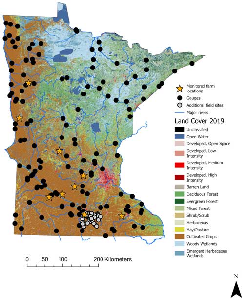
Figure 1 Locations of (1) 143 gauged stream and river watersheds intensively sampled for SRP and flow (total n= 22 750 samples) at the watershed outlet during 2007–2021 (black dots; n= 143). Data from these sites were used to evaluate SRP transport behavior and understand drivers of late-summer SRP. (2) Farm fields with tile outlet water quality available (collected between 2011–2021; orange stars; n= 10) used to estimate seasonal SRP concentrations for tile outlets as a point of comparison with riverine SRP concentrations. (3) Ditch, stream, and river sites sampled during summer low-flow conditions in 2014 (gray dots; n= 33). Data from these sites were used to quantify late-summer SRP concentrations in smaller-order systems. Note that two farm fields (known as RW1N and RW1S) are located in close proximity to each other and so appear to be one location on the map; this location is noted with a white arrow.

2.2 Overview of study data

For this study, we utilized three independent datasets (Fig. 1):

1. SRP concentration and discharge data (total n= 22 750 flow-matched water chemistry samples) collected for 143 gauged stream and river watersheds monitored by the state of Minnesota's Watershed Pollutant Load Monitoring Network (https://public.tableau.com/app/profile/mpca.data. services/viz/WatershedPollutantLoadMonitoringNetworkWPLMNDataViewer/ProgramOverview, last access: 23 October 2023) between 2007–2021. These data were used to evaluate SRP transport behavior and understand drivers of late-summer SRP.

2. SRP concentration and discharge data available for 10 tiled farm fields across the state, collected between 2011–2021 by the Discovery Farms Minnesota program (https://discoveryfarmsmn.org/, last access: 17 March 2023). These data were used to estimate seasonal SRP concentrations for tile outlets as a point of comparison with riverine SRP concentrations.

3. SRP grab samples collected during low-flow conditions in late summer of 2014 for an additional set of ditch, stream, and river sites (n= 33; Dolph et al., 2017a (https://conservancy.umn.edu/handle/11299/189907, last access: 27 March 2023)). These data were used to provide additional information about SRP concentrations in smaller-order systems that were underrepresented among gauged watersheds.

All data analyses were performed in R (R Core Team, 2023). The study data and R scripts used for data analysis are available at https://doi.org/10.5281/zenodo.13936951 (Dolph, 2024).

2.3 Water quality data from stream and river gauges

We used paired SRP and daily discharge data from 143 gauged stream and river watersheds (Fig. 1) monitored by Minnesota's Watershed Pollutant Load Monitoring Network (WPLMN; note that the WPLMN also refers to SRP as “dissolved orthophosphate”). The total number of samples across all gauged watersheds was 22 750. Periodic water samples and continuous-flow data were collected by the Minnesota Pollution Control Agency (MPCA) throughout the year at major watershed sites (watershed areas greater than ∼ 4000 km²) and during the period of ice-out through 31 October at smaller subwatershed sites (MPCA, 2015). Water quality sampling efforts were conducted approximately biweekly, with more intensive sampling focused on snowmelt and storm events, resulting in observations distributed across the range of flows observed at each site (average no. of samples per year = 25 for subwatersheds and 35 for major watersheds; MPCA, 2015). The 143 gauged sites we selected for this study had > 20 water chemistry samples collected across the sampling period (2007–2021). The median number of water quality samples per site across the whole time period was 120 (min = 21, max = 478). To determine detection limits, we inspected the data for repeated minimum concentrations and assigned detection limits equal to those minimum concentrations.

Watershed areas for gauged stream and river sites were assembled from multiple sources, including existing watershed delineations (n= 11 watersheds) available from USGS (2012) and previously delineated watersheds (n= 65 watersheds) from Dolph et al. (2019), or were delineated anew as part of the current study (n= 68 watersheds). For newly delineated watersheds, we used gauge locations provided by the Minnesota Department of Natural Resources and the Minnesota Pollution Control Agency (2023) as pour points, and we used existing flow direction and flow accumulation rasters available from the NHDv2Plus dataset (USEPA, 2019) to delineate watersheds using the Spatial Analyst toolbox in ArcGIS Pro (Esri, 2022). Watersheds were inspected visually and manually corrected for inaccuracies in delineation. Across all gauged sites, watershed area ranged from 20 to 29 145 km² (mean = 1996 km²).

2.4 Farm tile outlets

We used SRP concentration and discharge data from tile outlets draining 10 farm fields across the state, measured between 2011–2021 (Fig. 1). These tile outlets are monitored by the Discovery Farms Minnesota (DFM) program (https://discoveryfarmsmn.org/, last access: 17 March 2023). The DFM program is a farmer-led water quality research and educational program with the goal of collecting water quality information under real-world conditions to support the development of better farm management decisions. During the time of data collection, all monitored farm fields were planted in corn and soybean row crops grown in rotation. Two sites (WR1 and ST1) included dairy operations, and two sites (BE1 and DO1) included swine finishing in addition to row crops. Swine finishing is the final stage of pig farming, where young pigs are fed until they reach market weight.

The drainage areas for monitored farm fields ranged from 10 to 160 acres (mean = 97 acres). Farm field soil textures ranged from poorly drained silty clay loam to well-drained loam. Three of the farms (MC1, RE1, and WR1) each had one surface inlet to the tile drainage system. All other inlets were subsurface. One farm (NO1W) had monitoring data available for two separate fields (NO1W-N and NO1W-S). Water quality and flow data collection is described in detail by MDA (2021). Briefly, tile outlets were monitored continuously for flow (15 min interval) via area velocity sensors installed in the tile drains that measured both stage and velocity. Water quality samples were collected by ISCO 6712 automatic samplers on an equal-flow increment (EFI) composite basis whenever tile outlets were flowing. Water quality samples were composited every 125 mL. Following a runoff event, water quality samples were collected and promptly transported to a state contract lab and measured for dissolved orthophosphorus (i.e., SRP), along with other water quality constituents. From continuous-flow and composited-sample SRP concentrations, we calculated a daily flow-weighted SRP concentration (daily C) as follows: (1) multiply composite concentrations by paired continuous-flow measures to estimate continuous (15 min) loads, (2) sum composite-sample loads into daily loads, and (3) divide daily load by summed daily flow to compute a daily flow-weighted concentration (in mg L⁻¹). Seasonal SRP concentrations were calculated by taking the mean of the daily SRP concentrations for each tile outlet during each season (early winter: November–December; late winter: January–March; spring: April–May; early summer: June–July; late summer: August–September; fall: October).

2.5 Additional field sites

Among gauged stream and river watersheds, small-order systems (especially first- through third-order ditches and streams) are underrepresented relative to their prevalence across the landscape. To get a better understanding of SRP concentrations in smaller-order systems, we also examined late-summer low-flow SRP concentrations collected from 33 agriculturally dominated ditches, streams, and mid-sized rivers in the Le Sueur River basin, Minnesota (Fig. 1). Data for these sites are part of a larger publicly available field dataset (https://doi.org/10.13020/D6FH44, Dolph et al., 2017a) for the region and are described in detail by Dolph et al. (2019). Briefly, SRP concentrations were determined for grab water samples collected from 33 sites during low-flow conditions in August of 2014. Flow conditions at the time of sampling were characterized by flow at the gauged outlet of the major HUC8-scale watershed from which samples were collected (i.e., the Le Sueur River basin) based on daily discharge data available from Minnesota Department of Natural Resources (MNDR; https://www.dnr.state.mn.us/waters/csg/index.html, last access: 25 January 2016). Although flow at watershed outlets is not precisely representative of flow conditions further upstream in the basin, we have shown previously that discharge conditions across study sites scaled reasonably well with drainage area (Dolph et al., 2017b). We sampled on 14, 17, 20, and 26 August 2014, during which time flow conditions at the watershed outlet ranged between the 19–25th percentiles of all daily flows available for this watershed. Sites were categorized as ditches, perennial streams and rivers, or intermittent streams and rivers according to their designation in the NHDPlusv2 (USEPA, 2019).

2.6 Low-flow conditions

Part of our aim in this study was to identify whether in-channel dynamics, such as the in-stream release of legacy P, may affect stream and river SRP concentrations and transport behavior. Thus, we sought to identify low-flow conditions where we assumed that in-channel processes were likely to dominate P dynamics. We identified low-flow conditions as those falling within the lowest 25 % of all daily discharge conditions measured for each watershed during the period of record for that gauge. We defined seasons as follows: early winter (November–December), late winter (January–March), spring (April–May), early summer (June–July), late summer (August–September), and fall (October). We defined these seasons in approximate relation to the agricultural growing seasons in our study region, with spring corresponding to when crops are planted, summer corresponding to when crops grow rapidly, fall corresponding to when dominant crops (corn, soybeans) are harvested, and winter corresponding to when crops are dormant. We divided winter into early winter, which is when snow accumulates and generally does not melt, and late winter, which is associated with snowmelt. We divided summer into early summer, which is when conditions are generally wetter and crops experience rapid growth, and late summer, which is when climate conditions are generally drier and warm-season crops mature rapidly.

We calculated the mean SRP during low-flow conditions for each gauged watershed in each season for gauges that had a minimum of three SRP samples collected during low-flow conditions in that season. Note that not all gauged watersheds had three or more SRP samples collected during low flows in each season (Table A4 in the Appendix); thus, the number of gauged watersheds with mean low-flow SRP values available for analysis was different during each season (this parallels the availability of low-flow conditions across seasons, with low flows being most common during late summer compared to during other seasons).

We hypothesized that low-flow SRP concentrations could be substantially affected by one or all of the following: tile outlet concentrations, wastewater treatment plant discharges, or riverine legacy P stores. To help discern these influences, we compared low-flow riverine SRP concentrations to tile outlet concentrations. In addition, we evaluated low-flow riverine SRP concentrations for gauged watersheds relative to the wastewater treatment plant density (sites per km²) in the watershed. Wastewater treatment plant density estimates were obtained from the US EPA StreamCat Dataset and were based on wastewater treatment plants listed in the EPA's Facility Registry Services and National Pollutant Discharge Elimination System (Hill et al., 2016). We also evaluated low-flow riverine SRP concentrations relative to the percentage of cropland land use in gauged watersheds to examine the assumption that agricultural land use and the associated past and current P inputs might drive the supply of riverine P. Cropland land use estimates were also obtained from the StreamCat Dataset and were based on the 2019 National Land Cover Database (Dewitz, 2021).

2.7 Influence of late-summer low flows on concentration–discharge relationships

We evaluated the relationship between SRP concentration (C) and discharge (Q) using the power-law relationship in Eq. (1):

$$\begin{array}{}\text{(1)}& C=a{Q}^b,\end{array}$$

where the curve's coefficient (a) and exponent (b) are representative of the degree, direction, and rate at which SRP is transported as a function of streamflow. Alternatively, this equation can be expressed in log–log scale as Eq. (2):

$$\begin{array}{}\text{(2)}& \log \left(C\right)=b\log \left(Q\right)+\log \left(a\right),\end{array}$$

where b is the slope of the linear log–log relation, and log(a) is the y intercept. Normalizing Q by the geometric mean of discharge (Q_GM) shifts the center of mass of the log-transformed Q data to the y intercept, allowing for comparison of rating curves among different watersheds (Warrick, 2015). We performed linear regression of log-transformed SRP concentrations based on log-transformed normalized discharge using Eq. (3):

$$\begin{array}{}\text{(3)}& \log \left(C\right)=b\log (Q/Q_{\mathrm{GM}})+\log \left(a\right).\end{array}$$

All regressions were performed in R (R Core Team, 2023). We evaluated the fit of the power-law relationship for all gauged watersheds using the significance value p, slope b, and R² of the linear regression.

The slope b of this relationship describes the per-unit increase in concentration as discharge increases. Concentrating relationships (b > 0) imply that higher flows are mobilizing more of a waterborne constituent, particularly through erosion or greater landscape connectivity. Diluting relationships (b < 0) suggest that constituents are source-limited or that relatively consistent inputs are diluted by greater discharge (Godsey et al., 2009). When b is near 0, C–Q relationships may be either chemostatic (i.e., relatively constant concentrations across the range of discharge conditions) or chemodynamic (i.e., concentrations are highly variable across the range of discharge conditions but are not linearly related to flow). Chemostatic behavior has been observed for mineral weathering products or for constituents with large legacy sources like nitrate (Godsey et al., 2009; Basu et al., 2010; Musolff et al., 2015), whereas chemodynamic behavior may indicate that biogeochemical processes such as sorption and/or desorption, biotransformation, or oxidation and/or reduction strongly affect nutrient transport behavior (e.g., Wanner et al., 1989). To distinguish between these two behaviors, we evaluated the coefficient of variation of C relative to the coefficient of variation of Q (CV${}_C/{\mathrm{CV}}_Q$). A CV${}_C/{\mathrm{CV}}_Q$ ≪ 1 suggests that concentrations are relatively constant compared to variability in flow, indicating chemostatic behavior. By contrast, a larger CV${}_C/{\mathrm{CV}}_Q$ indicates chemodynamic behavior (i.e., comparatively large variations in concentration relative to variation in flow). Thompson et al. (2011) suggested that CV${}_C/{\mathrm{CV}}_Q$ values of ≈ 0.3 could be used as a threshold to identify chemostatic vs. chemodynamic behavior.

To determine the influence of low-flow conditions in late summer on the nature of the C–Q relationships for all watersheds, we refit power-law relationships to all watersheds after excluding SRP samples that were collected during late-summer low-flow conditions. We compared regression parameters (p, slope b, and R²) before and after withholding samples collected during late-summer low-flow conditions to determine if these samples had a widespread effect on C–Q relationships for SRP across gauged watersheds.

2.8 Regression analysis

2.8.1 Random forest models

We used random forest modeling to identify possible predictors of SRP during low-flow conditions in late summer for gauged stream and river watersheds. Random forest regression is a nonparametric ensemble learning method that utilizes predictions from multiple decision trees to improve model accuracy. Each tree is composed of branches (“nodes”) representing yes–no questions where features (i.e., predictive variables) are used to split the dependent variable into two groups that minimize in-group variability and maximize between-group variability. We selected a random forest approach because these models require few assumptions about data structure (i.e., data need not conform to assumptions of classical statistics such as linearity, normality, and constant variance), are robust in relation to outliers, and generally perform as well as or better than other data-intensive approaches (Hagenauer et al., 2019). The use of random forest models also allows for the identification of predictors that are important to model accuracy using measures such as condition permutation importance and post hoc partial-dependence plots (see additional details below).

2.8.2 Predictor variables

Predictor variables for random forest (RF) models were assembled from the US EPA StreamCat Dataset (https://www.epa.gov/national-aquatic-resource-surveys/streamcat-dataset, last access: 5 February 2024). The StreamCat Dataset contains information for over 600 different environmental metrics linked to individual stream reaches in the NHDv2Plus dataset (Hill et al., 2016). These metrics summarize, at the catchment and watershed scales, diverse geospatial attributes – including aspects of land cover, impervious surfaces and road density, soil type, point source and nutrient inputs, and climatic factors (temperature and precipitation), among others – draining into each reach. Catchments (i.e., local drainage areas) include the immediate land area draining into each individual stream reach in the National Hydrography Dataset (NHD) excluding areas draining to upstream reaches; watersheds include the entire land area draining into each stream reach. The StreamCat Dataset contains land use data for catchments and watersheds summarized from the National Land Cover Database (NLCD) for multiple years. We used only land cover attributes from the 2019 iteration of the NLCD (Dewitz, 2021). To supplement this dataset, we derived estimates of tile density (i.e., area tiled per area watershed) for each gauged watershed using estimates of tiled areas (30 m resolution) from Valayamkunnath et al. (2020). Prior to developing a random forest model, we excluded predictors from the StreamCat Dataset that did not contain useful information (i.e., all rows = 0). We also excluded attributes where information was missing (“NA”) for > 20 % sites. Some of the remaining attributes still contained some missing values. Because random forest models cannot handle missing values in predictor variables, we used the missRanger package in R (Mayer, 2023) to impute the remaining missing values for the training and testing datasets. In total, we used 253 predictor variables in the model after excluding variables that did not provide useful information (i.e., that were all 0 s or had too many missing values), that did not match the timing of our dataset (i.e., land cover data from years other than 2019), or that were not especially relevant (e.g., variables describing forest fire intensity or extent). Prior to random forest modeling, we normalized (i.e., centered and scaled) numeric attributes to have a mean of 0 and a standard deviation of 1.

2.8.3 Model tuning and selection

We developed the random forest model to predict mean SRP during late-summer low conditions based on data for 127 gauged watersheds. Only 128 of the 143 total gauged watersheds in the study had ≧  3 SRP samples collected during late-summer low-flow conditions and were therefore used to calculate mean SRP values. Prior to model development, we excluded one additional site from the testing dataset (Buffalo Creek near Glencoe, MN) that had a mean SRP value for late summer that exceeded the range of SRP values in the training dataset (see Fig. A1). To develop the RF model, we used the same general approach to random forest modeling described in detail by Dolph et al. (2023). Data were split randomly into independent model training (70 %, n= 88) and model testing (30 %, n= 39) datasets. Using the training dataset and the ranger package in R (Wright and Ziegler, 2017), we applied 10-fold cross-validation to tune model hyperparameters across a range of possible values. K-fold cross-validation can assist in avoiding model over-fitting and works by partitioning training data into K equal-sized “folds” (in our case, 10). The model is iteratively trained on various combinations of tuning hyperparameters across K-1 folds, leaving the remaining fold to evaluate model performance for each combination. The hyperparameters selected for tuning were as follows: mtry (i.e., number of variables randomly sampled as candidates at each split) and min_n (i.e., the minimum number of data points in a node). The tree hyperparameter (i.e., number of trees) was set to 1000 across all models. We defined a grid of 20 potential combinations of hyperparameters using the tune_grid() function from the tidymodels collection of packages in R (Kuhn and Wickham, 2020). This approach draws hyperparameter values semi-randomly from the parameter space such that the various combinations cover the whole space of potential values. We selected hyperparameter values using out-of-bag (OOB) RMSE and R² for the associated models. Once hyperparameter values were tuned, we reran the random forest model using the randomForest package (Liaw and Weiner, 2002) to create a randomForest object that was compatible with our selected measure of predictive variable importance (conditional permutation importance; see next paragraph). We evaluated overall model performance using R² and RMSE between the predicted and observed SRP values in the independent test dataset (comprising 30 % of the original dataset).

2.8.4 Variable importance

We used conditional permutation importance (CPI) to evaluate the importance of predictors to model performance. CPI aims to capture the dependence between a predictor and the response variable based, conditionally, on the values of all other predictors. CPI can be used to assess how much each variable contributes to accurately predicting the response variable, given what we know from all other predictive variables. We implemented the CPI approach from the permimp package in R (Debeer et al., 2021). In permimp, a threshold value, equal to 1 minus the p value for the association between predictor variables, is used to determine whether to include a predictor in the conditioning for the predictor of interest. We used the default value for the threshold parameter in permimp (0.95; Debeer et al., 2021).

While the CPI method can rank predictors in terms of their importance to model accuracy, it does not convey information about the nature of the relationship between predictor variables and late-summer SRP concentrations. To visualize these relationships, we created partial-dependence plots (PDPs) using the partialPlot function in R (part of the randomForest package, Liaw and Weiner, 2002). These plots illustrate the change in predicted SRP concentration when the values of one predictor are changed while all other predictors are kept constant at their original values (Greenwell, 2017). We generated PDPs for the top 15 predictor variables identified as being most important by the measure of CPI.

3 Results

3.1 SRP concentrations at gauged watersheds during low flow

Across gauged watersheds, we expected SRP concentrations under low-flow conditions to differ depending on the extent of historic and current P inputs associated with anthropogenic land use. Most gauged watersheds in our study region (90 %, n= 128) were substantially impacted by either agricultural or urban land use (defined here as watersheds with ≧  50 % crop cover and/or ≧  10 % high-intensity urban land use). The remaining watersheds (n= 15) were characterized as “less impacted”.

Among watersheds with substantial agricultural or urban influences, mean low-flow SRP concentrations were highest in late winter and were lowest in spring and then increased progressively through early summer, late summer, fall, and early winter (Table 1).

Table 1 Mean, minimum, and maximum low-flow SRP concentrations (mg L⁻¹) for more heavily impacted gauged watersheds (≧  50 % crop cover and/or ≧  10 % high-intensity urban land use) and less impacted gauged watersheds (< 50 % crop cover and/or < 10 % high-intensity urban land use) across seasons.

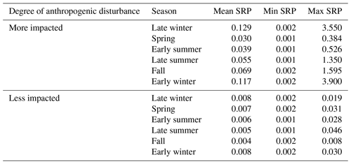
However, there was large variation (3–4 orders of magnitude) in low-flow SRP concentrations across sites in any given season (range across all samples = 0.001–3.9 mg L⁻¹). For less impacted sites, seasonal low-flow SRP concentrations were also highest, on average, during late winter, although the absolute concentrations were much lower than for more heavily impacted sites. In contrast to more heavily impacted sites, mean low-flow SRP concentrations at less impacted sites dropped in spring and stayed steady through summer and then dropped slightly again in fall. Less impacted sites showed comparatively low SRP concentrations and lower variability in low-flow SRP concentrations across sites or seasons (range of 0.001–0.046 mg L⁻¹).

3.2 Influences of wastewater treatment facilities (point sources) on riverine SRP concentrations at low flow

Mean SRP concentrations at low flow for gauged watersheds were significantly related to the density of wastewater treatment plants in the watershed during early winter, late winter, late summer, and fall but not in spring or early summer (Fig. 2). Part of the discrepancy across seasons may have been caused by the fact that few watersheds with a high density of wastewater treatment plants were sampled during low flows in spring and early summer. The relationship between mean low-flow SRP and wastewater treatment plant density was strongest in early winter (though still somewhat weak overall; R²= 0.26) and comparatively weaker in other seasons (Table A1). These relationships were largely driven by watersheds where the density of wastewater treatment plants was comparatively high (> 0.005 sites km⁻²). When watersheds with a wastewater treatment plant density > 0.005 sites km⁻² were excluded, we observed a persevering very weak significant positive relationship between wastewater treatment plant density and mean low-flow SRP during late summer and late winter (R²= 0.06 and 0.10, respectively) but not during any other season (see Table A1).

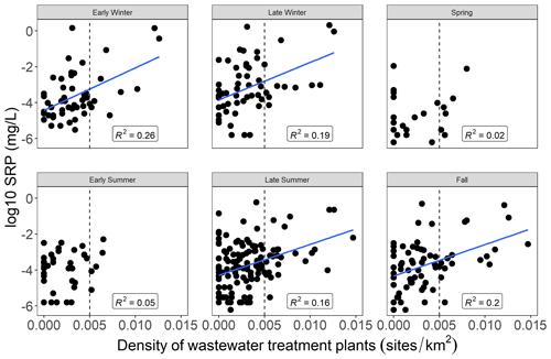
Figure 2 Relationship of SRP concentrations at low flows (log scale) in gauged watersheds to the density of wastewater treatment plants (sites km⁻²) in the watershed by season. Blue lines indicate statistically significant linear regressions (p < 0.05). Linear regression statistics are shown in Table A1. The dashed line indicates a wastewater treatment plant density of 0.005 sites km⁻². Note that not all gauged watersheds had sufficient samples collected during low flows in each season to generate mean values; thus, the number of gauged watersheds with low-flow mean SRP values available was different during each season.

3.3 Riverine SRP at low flows in relation to agricultural land use

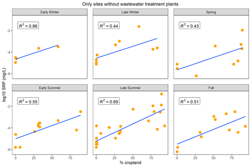
We observed consistent and positive relationships between agricultural land use (% cropland) and mean low-flow SRP concentrations across gauged watersheds during all seasons, with the strongest relationships occurring during late summer and late winter (Fig. 3; Table A2). When we examined only sites without wastewater treatment plant influence, these relationships appeared to be even stronger, as evidenced by increased R² values (Fig. 4; Table A2). The strongest correlations were evident in late summer and early winter (R² of 0.69 and 0.86, respectively; Fig. 4). However, it should be noted that the sample size for early winter was small (n= 5), which may have inflated the R² value for this season.

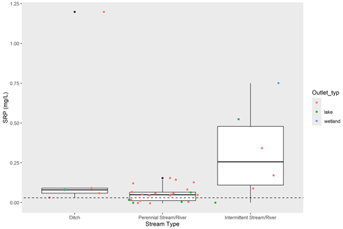
Figure 3 Mean low-flow SRP concentrations across gauges (log scale) in relation to percentage crop cover by season. Color scale indicates density of wastewater treatment plants in the watershed. Relationships in all seasons were significant and positive. Linear regression statistics are shown in Table A2.

Figure 4 Mean low-flow SRP concentrations across gauges (log scale) in relation to percentage crop cover by season for sites with no wastewater treatment plant influence. Relationships in all seasons were significant and positive. Linear regression statistics are shown in Table A2.

3.4 SRP concentrations at tile outlets

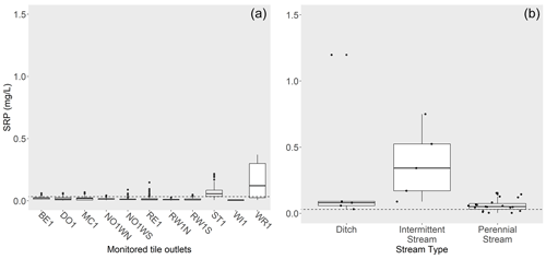
Across tile outlets for 10 conventionally farmed fields (corn–soybean rotation), the mean SRP concentration of tile drainage was highest in late winter (mean SRP = 0.131 mg L⁻¹) and was lowest in early and late summer and early winter (mean SRP = 0.03 mg L⁻¹; Table 2). Two sites (WR1 and ST1) included dairy operations, and two sites (BE1 and DO1) included swine finishing in addition to row crops. The two dairy-influenced farm fields (WR1 and ST1) had notably higher tile SRP concentrations across all seasons relative to other sites. Three sites (MC1 RE1, and WR1) had one surface inlet to the tile system (all other inlets were subsurface). These sites appeared to have higher mean SRP concentrations in late winter (coinciding with snowmelt) and early summer (in the case of WR1), but of the surface inlet sites, only WR1 (the dairy farm site) had higher mean SRP concentrations in late summer.

Table 2 Mean flow-weighted daily SRP concentrations (mg L⁻¹) from farm tile outlets by season. Tile outlet data were collected from 10 farms between 2011–2021. Note that one farm field (NOW1) had two tile outlets (NOW1-N and NOW1-S) that drained different areas of the same field.

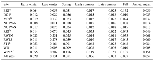
Early winter: November–December. Late winter: January–March. Spring: April–May. Early summer: June–July. Late summer: August–September. Fall: October. ^a Farms included dairy operations. ^b Farms included a surface inlet to the tile drainage system. ^c Farms included swine finishing.

3.5 Riverine SRP at low flows compared to tile concentrations

We evaluated SRP during low-flow conditions for each gauged watershed in each season (Table A3) and compared these riverine SRP values to SRP concentrations in monitored tile outlets. Note that not all gauged watersheds had sufficient samples collected during low flows in each season to generate mean values (Table A4); thus, the number of gauged watersheds with available mean low-flow SRP values was different during each season. Comparisons for late winter, spring, and late summer are shown in Fig. 5 (only a subset of seasons are shown for improved clarity in data visualization; similar figures for early winter, early summer, and fall are shown in Fig. A2).

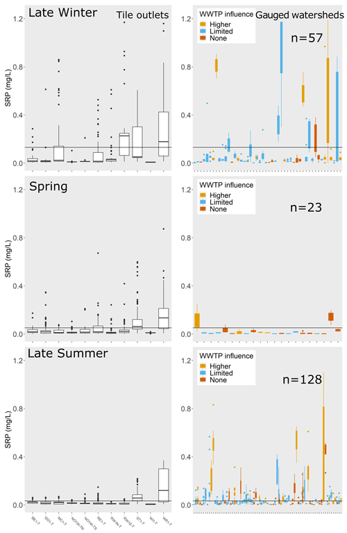
Figure 5 SRP concentrations (mg L⁻¹) for tile outlets and during low-flow conditions for gauged watersheds by season. Only a subset of seasons are shown for improved clarity in data visualization; similar figures for the remaining seasons are shown in Fig. A2. The horizontal line in each plot is the mean SRP concentration among tile outlets for that season. For gauged watersheds, the color of the boxplots indicates the degree of influence from wastewater treatment plants: light orange indicates wastewater treatment plant density > 0.005 sites km⁻², blue indicates wastewater treatment plant density < 0.005 sites km⁻² but greater than zero, and red indicates no wastewater treatment plant sites in watershed. The number of gauges for which low-flow data were available in each season is printed on the plot. To improve data visibility, the y axis for SRP was limited to a maximum of 1.25 mg L⁻¹, which eliminated a small number of outliers from the plots for tile outlets (n= 34 out of 11 079 records) and gauged watersheds (n= 16 out of 2696 low-flow records).

In early winter, 36 % of gauged watersheds (n= 18/50 sites for which low-flow data were available) exhibited SRP concentrations at low flows that were higher than mean tile SRP concentration. Six of these watersheds were characterized by a comparatively high wastewater treatment plant density (defined as > 0.005 sites km⁻²). In late winter, when tile SRP concentrations were highest, 23 % of gauged watersheds (n= 13/57) exhibited SRP concentrations at low flows that were higher than the mean tile concentrations. A minority of these sites (n= 3/13) had considerable wastewater treatment plant influence (wastewater treatment plant density > 0.005 sites km⁻²). In spring, SRP concentrations during low-flow conditions were uniformly low across nearly all gauged watersheds. SRP samples collected during low-flow conditions were fairly uncommon, with only 23 watersheds having ≧  3 SRP samples collected during spring low flows. Of these, two sites (9 %) had SRP concentrations at low flows that were higher than the mean tile concentrations. In early summer (June–July), 28 % of sites (n= 11/40) had SRP concentrations at low flow that were higher than the mean tile concentrations. Two of these sites had considerable wastewater treatment influence. In late summer (August–September), 39 % of gauged watersheds (n= 50/128) had SRP concentrations at low flow that were higher than the mean tile concentrations, and 16 of these sites had considerable wastewater treatment influence. In fall (October), 35 % of gauged watersheds (n= 24/68) had SRP concentrations at low flow that were higher than the mean tile concentrations; eight of these sites had comparatively higher wastewater treatment plant density.

3.6 Low-flow SRP concentrations from additional field sites

Among gauged stream and river sites, small-order systems (especially first- through third-order ditches and streams) were underrepresented relative to their prevalence across the landscape. These smaller-order systems are also less likely to have substantial point source discharges. To get a better understanding of SRP conditions in smaller-order systems, we examined SRP concentrations collected from 33 agriculturally dominated ditches, streams, and mid-sized rivers in southern Minnesota during low-flow conditions in August 2014 (Dolph et al., 2017). During this sampling event, SRP concentrations at most sites were higher than mean SRP concentrations from farm tile outlets (Fig. 6). Mean SRP concentrations in late summer were highest in ditches and intermittent streams (0.19 mg L⁻¹ and 0.30 mg L⁻¹, respectively).

Figure 6 SRP concentrations (mg L⁻¹) among tile outlets (a) compared to sampled ditches (n= 5), intermittent streams and rivers (n= 6), and perennial streams or rivers (n= 22) and (b) during late-summer low-flow conditions. Dashed line shows mean SRP concentration for tile outlets in late summer.

3.7 C–Q relationships at stream and river gauges

When C–Q relationships were evaluated using all flow data for each gauge, the majority of gauged watersheds (72 %, n= 103) showed mobilizing behavior for SRP in relation to streamflow (i.e., significant positive slopes for the C–Q power-law relationship and CV${}_C/{\mathrm{CV}}_Q$ > 0.3; Fig. A3). Mobilizing behavior for bioavailable P ranged from very weak (R²= 0.01) to comparatively strong (R²= 0.68). Watersheds with positive SRP–Q relationships were located predominantly in the agriculturally dominated regions of the state (the southern and western parts of the state corresponding to the southern part of the Upper Mississippi River basin, the Minnesota River basin, the Driftless Area in the southeast, and the Red River basin; Fig. 7). Chemodynamic behavior (non-significant slopes for the C–Q power-law relationship and CV${}_C/{\mathrm{CV}}_Q$ > 0.3) was observed for 24 % (n= 34) of sites, most of which are located in the central and northeastern parts of the state dominated by forest and wetland cover (Fig. 7). A small number of sites (n= 4, 3 %) showed diluting behavior for SRP, as defined by significant negative slopes for the C–Q power-law relationship and CV${}_C/{\mathrm{CV}}_Q$ > 0.3. Two of these sites showed considerable wastewater treatment plant influences (wastewater treatment plant density > 0.005 sites km⁻² Table A3). Three sites (2 %) showed chemostatic behavior for SRP transport, as defined by a CV${}_C/{\mathrm{CV}}_Q$ ≦ 0.3.

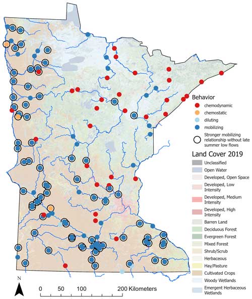
Figure 7 Transport behavior of SRP in relation to flow (Q) for gauged watersheds (n= 143). Dots indicate gauge locations. The color of the dots indicates transport behavior diagnosed by slope b of the C–Q power-law relationship and CV${}_C/{\mathrm{CV}}_Q$. Mobilizing behavior is indicated by dark-blue dots (n= 103), chemodynamic behavior is indicated by red dots (n= 34), diluting behavior is indicated by light-blue dots (n= 4), and chemostatic behavior is indicated by orange dots (n= 3). Sites with a stronger mobilizing relationship (i.e., an increase in slope b) when late-summer low flows are excluded are shown as open circles (n= 78). Land cover is based on the 2019 National Land Cover Database.

When low-flow samples from late summer were removed, 54 % of gauged watersheds (n= 78) exhibited an increase in the slope of the mobilizing relationship between SRP and Q (Fig. 7; Table A5). For these sites, slopes of the C–Q relationships increased by 23 %, on average, after late-summer low-flow samples were excluded (the range, in percentage slope increase, was 0. 1%–273 %). In other words, mobilizing behavior for SRP was stronger when these late-summer low-flow conditions were excluded. Examples of this phenomenon for four different gauged watersheds are shown in Fig. 8, where the slope of the C–Q relationship is steeper when late-summer low-flow samples were excluded and comparatively flatter when they are included. Watersheds where late-summer low flows modulated (flattened) the slope of the C–Q relationship for SRP were again located predominantly in the agriculturally dominated regions of the state (Fig. 7).

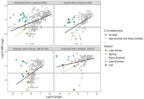
Figure 8 Example watersheds where low flows in late summer modulate the slope of the C–Q relationship for SRP. Low-flow samples are shown as colored points, where the color indicates the season in which they were collected. All other samples are shown in gray. When all data are included, the slope of the overall C–Q relationship is reduced (solid line) compared to slopes for analyses with late-summer low-flow samples omitted (dashed line), indicating stronger mobilizing behavior.

3.8 Regression analysis to identify drivers of elevated SRP concentrations in late summer

The final selected hyperparameters for the random forest model based on model tuning with 10-fold cross-validation for this dataset were mtry = 7, trees = 1000, and min_n = 6. The evaluation of the predicted vs. actual late-summer SRP for the independent test dataset indicated a model RMSE of 0.10 and an R² of 0.41 (Fig. A4). On average, the random forest model underestimated actual mean SRP concentrations during late-summer low flows compared to actual measured values among test sites (mean of estimated −  true values = −0.005). However, this negative bias was driven by poor predictive model performance for three sites with exceptionally high mean SRP concentrations of 0.293, 0.525, and 0.526 mg L⁻¹ (Fig. A4). For the remaining test sites (all with mean SRP < 0.2 mg L⁻¹), the predictive bias (mean of estimate − true values = 0.02) was actually positive. For most sites, in other words, the random forest model overestimated mean late-summer SRP concentrations compared to measured values.

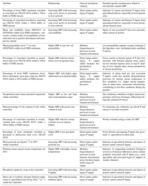
The top 15 predictors of model performance are shown in Fig. 9. Importance values for all predictors are shown in Table A6. Partial-dependence plots for these top predictors (Fig. 10) showed that higher SRP during late-summer low-flow conditions was associated with higher cropland land use in riparian areas, various soil characteristics (higher soil erodibility, lower soil permeability, higher soil clay content), greater agricultural intensity (higher pesticide use, higher phosphorus uptake by crops, higher fertilizer application rates), more urban land use in riparian areas, lower woody wetlands and mixed forest in riparian areas, lower grassland land use in watersheds, lower surplus precipitation in the watershed (precipitation minus evaporation), and higher stream temperatures. Table 3 summarizes possible mechanisms linking these attributes to riverine SRP concentrations.

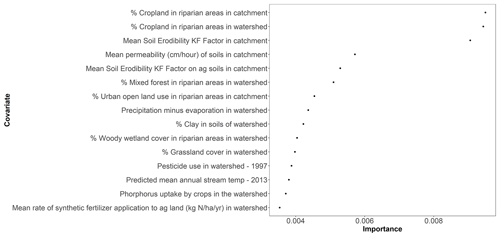
Figure 9 Conditional permutation importance (CPI) values for the top 15 predictors in the random forest model for late-summer SRP during low flows and in stream and river gauges. CPI is a measure that can be used to assess how much each variable “adds” to accurately predicting the response variable, given what we know from all other covariates. Importance values for all attributes are given in Table A6.

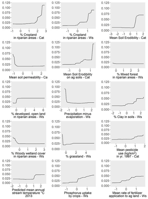
Figure 10 Partial dependence (y axis indicates the change in predicted SRP value) for each of the 15 most important predictors of model performance. Partial dependence shows the change in the response variable (late-summer low-flow SRP) when each predictor of interest is varied while all other predictors stay constant. “Ws” refers to predictors summarized at the watershed scale, and “Ca” refers to predictors summarized at the catchment scale. All predictor variables are from the US EPA StreamCat Dataset (Hill et al., 2016).

Table 3 Possible mechanisms linking random forest model predictor variables to late-summer SRP concentrations during low-flow conditions for the top 15 attributes identified as being most important to the performance of the random forest model. All attributes are from the US EPA StreamCat Dataset.

4 Discussion

In this study we observed that between one-third to one-half of the gauged watersheds in Minnesota exhibited SRP concentrations during late-summer low flows that were above previously identified thresholds for eutrophication of 0.02–0.04 mg L⁻¹ for freshwater environments (Zeng et al., 2016; Poikane et al., 2021) (34 % were above a threshold of 0.04 mg L⁻¹, and 53 % of watersheds were above 0.02 mg L⁻¹). One avenue for future research is to investigate how the timing and duration of elevated summer SRP concentrations affect local and downstream eutrophication outcomes. On the one hand, the large majority of annual P export by load is likely to occur under high-flow conditions in late winter and spring (Dolph et al., 2019; Schilling et al., 2020). However, the release of highly bioavailable P during hot, dry summer periods when conditions are optimal for algal growth in lakes and rivers may also drive increased eutrophication risk, resulting in outcomes such as increased occurrence of harmful algal blooms (Paerl and Huisman, 2008). As climate change is expected to result in increased prolonged periods of drought and heat during summer in the Upper Midwest (Wilson et al., 2023), the effects of elevated bioavailable P at low flows could be extended for longer parts of the season.

We also observed that, for more than half of the gauged watersheds we studied (54 %), elevated SRP concentrations during low flows in late summer dampened C–Q relationships which would have otherwise appeared to be more strongly mobilizing across other seasons and flow conditions. Strongly mobilizing relationships are indicative of landscape connectivity as a key driver for SRP export (Musolff et al., 2015), with flow accumulation and riparian areas identified as critical source areas for SRP (Casquin et al., 2020; Dupas et al., 2023). Thus, for many of the sites we studied, connectivity appears to be important to SRP export during winter, spring, and early summer and under moderate- to high-flow conditions at all times of year. During late-summer low flows, by contrast, other in-channel dynamics may cause riverine C–Q patterns to deviate from linear relationships (Meybeck and Moatar, 2012). Below, we discuss possible mechanisms that may contribute to comparatively high SRP concentrations during late-summer low-flow conditions in the streams and rivers of our study region.

4.1 Drivers of SRP during late-summer low flows

Overall, our analysis shows that landscape drivers that govern diffuse P inputs and legacy P supply in the river network, as well as wastewater inputs and biogeochemical processes, are associated with high late-summer SRP concentrations during low flows at many anthropogenically dominated sites. Crop cover was strongly and directly related to SRP concentrations during low-flow conditions in all seasons, and crop cover in riparian areas at the local catchment and watershed scales was one of the top two most important variables with regard to the performance of the random forest model used to predict late-summer low-flow SRP concentrations. Other top variables with regard to model performance included aspects of agricultural intensity at the watershed or catchment scale (pesticide use, phosphorus uptake by crops, and fertilizer application), as well as urban land use in riparian areas. The importance of these variables points to historic and ongoing inputs of P arising from intensive and/or industrial agricultural and urban land uses that have resulted in the accumulation of legacy P in riverine channels, which can potentially be released under environmental conditions such as warm temperatures, low oxygen, and variable moisture. Conversely, greater mixed forest or woody-wetland land use in riparian areas was associated with lower SRP concentrations during late-summer low flows, perhaps because these environments may act as sinks for bioavailable P (Ury et al., 2023). Overall, it is notable that land use in riparian areas showed up as one of the top variables of importance with regard to model performance, suggesting that near-channel environments (and, therefore, potentially, near-channel management practices) may be important in regulating elevated SRP during late-summer low flows. Lastly, both geologic and climatic variables (soil erodibility, soil permeability, clay content of soils, mean annual stream temperatures, and precipitation minus evaporation) were also identified as important in the random forest model in terms of predicting late-summer low-flow SRP, suggesting that environmental factors which mediate biogeochemical processes are also likely to play an important role in driving late-summer riverine SRP concentrations.

Interestingly, SRP concentrations during late-summer low-flow conditions in anthropogenically dominated watersheds often exceeded tile SRP concentrations. Although tile drainage is known to represent a key input of P to river networks (Smith et al., 2015), it may be that in-channel dynamics beyond tile concentrations drive variability in SRP concentration during summer low flows. However, it is also important to note that the two tile outlets draining farms with dairy operations exhibited much higher SRP concentrations during late summer (and at all times of the year) compared to tile outlets draining fields characterized only by corn and soybean row crops. Thus, the prevalence of CAFOs and other animal agriculture operations is likely to strongly influence the contribution of tile drainage to riverine SRP concentrations. Three sites also had a surface inlet to their tile drainage system. These tile systems had comparatively high SRP during winter, spring, or early summer (depending on the site), which can likely be explained by the additional loss of sediment and nutrients to surface inlets during snowmelt on frozen and thawing soils (Feyereisen et al., 2015). However, the two surface-inlet-influenced sites without dairy operations exhibited SRP concentrations during late summer similar to those of other impacted non-dairy sites.

Wastewater treatment plant density did not rank among the most important predictors in our random forest model performance, and a substantial portion of sites (38 %) exhibited elevated SRP concentrations (above 0.02 mg L⁻¹) during late-summer low-flow conditions despite having limited or no wastewater treatment plant influence in their watersheds. However, the influence of wastewater on summer low-flow SRP was evident in the elevated SRP concentrations at sites with strong wastewater influence throughout most seasons (apart from spring, when low-flow SRP concentrations were nearly universally low, presumably due to rapid in-stream uptake or abiotic immobilization).

4.2 Biogeochemical processes and riverine SRP

Previous studies have identified a number of biogeochemical processes that can affect riverine concentrations of SRP at low flows. These processes include (1) the concentration of legacy P entering the stream via groundwater and/or streambed pore water, (2) the redox-driven release of P from stream sediments, and (3) the release of P resulting from mineralization of organic matter.

During low-flow conditions, groundwater and/or pore water can become proportionately dominant components of flow, with stores of legacy P in these sources contributing more strongly to overall riverine SRP. These groundwater sources can include tile drainage (Schilling et al., 2020; Rode et al., 2023) but can also include streambed pore water entering from the hyporheic zone via upwelling flow paths with P concentrations that are distinct and potentially higher than that of tile drainage (Vissers et al., 2023). Upwelling of P-rich pore water can be patchy and is likely to be controlled by hyper-local spatial and temporal conditions operating at the reach scale, such as the availability and extent of reducing vs. oxic conditions (e.g., Vissers et al., 2023).

SRP can also be released into river channels from stream sediments. Stream sediments often have the potential to buffer stream SRP concentrations by adsorbing P (Simpson et al., 2021). However, this buffering capacity will depend on sediment and stream characteristics, including sorption affinity; stream pH; exchangeable P concentration; sediment particle sizes; and seasonal variations in temperature, light, discharge, redox, primary productivity, stream respiration, and sediment inputs (Simpson et al., 2021). Seasonal release of SRP is commonly thought to occur via the reduction of Fe-, Mn-, or Al-oxyhydroxide-containing sediments under anoxic conditions, releasing PO${}_{\mathrm{4}}^{\mathrm{3}-}$. These anoxic conditions typically arise when flow velocities are low, when water and sediment temperatures increase, and when oxygen becomes depleted due to increased microbial activity. For example, Smolders et al. (2017) showed that high summer concentrations of bioavailable P for rivers in Belgium were likely to be explained by internal loading from legacy P that was released from sediments when dissolved oxygen concentrations were low and when P : Fe molar ratios in sediment were large.

Lastly, Jarvie et al. (2020) showed that, in a wetland–pond system, microbial respiration and the resulting mineralization of organic matter can also represent a source of bioavailable P under low-flow conditions in summer and fall. They found that SRP release was potentially related to drier and hotter conditions that could facilitate both higher rates of biomass accumulation and its subsequent breakdown via microbial processes. Presumably, this dynamic could also be at play for slow-moving ditches and streams in parts of our study region where water is sometimes nearly stagnant in summer. Under low-flow conditions and warm temperatures, ditches and streams may operate in ways that are similar to wetlands or other lentic waterbodies. The stream network is also populated with in-channel and riparian wetlands that may further affect ambient SRP concentrations. Felton et al. (2023) found elevated dissolved P concentrations along a longitudinal stream gradient where the channel intersected wetlands and concluded that locally elevated SRP could reflect P release from the decomposition of organic matter in wetland environments; however, in that study, elevated P concentrations did not persist downstream and were assumed to be rapidly assimilated or adsorbed to sediments.

Our findings provide some insight into the relative importance of these potential in-channel processes in determining seasonally elevated SRP concentrations at low flow. The importance of climate and geologic variables in the random forest model we used to predict late-summer low-flow SRP suggests that characteristics of stream sediments and/or climate-mediated biotic activity may play an important role in elevated SRP concentrations in late summer. Partial-dependence plots indicated that increased SRP during late-summer low flows was associated with the drier conditions (lower precipitation minus evaporation in gauged watersheds) and warmer conditions (higher predicted mean stream temperatures)¹. This finding could be consistent with the important role of biologically mediated processes, such as microbial respiration, that are affected by temperature and stream discharge. Microbial activity is important in both the decomposition of organic matter (i.e., mineralization) and the reduction of redoximorphic sediments (i.e., sediments containing Fe, Al, Mn), both of which can result in the release of SRP. The predicted mean stream temperature values used in this study were derived from Hill et al. (2013) and were themselves influenced by air temperature, soil permeability, agricultural and urban land use, stream slope, reservoirs, and watershed area. The positive relationship between stream temperature and late-summer SRP at low flow needs further investigation but could also be related to the greater influence of groundwater or to climate gradients that correspond to variations in biological activity or in land use and associated P inputs.

Soil erodibility was also identified as one of the most important variables with regard to random forest model performance, with partial-dependence plots showing higher SRP during late-summer low flows corresponding with greater soil erodibility in the local catchment. Eroded soils have long been understood to be a primary vector by which P enters river networks (Berhe et al., 2018). Recently, this understanding has been expanded to include eroded stream bank sediments as an additional driver of downstream P transport (Margenot et al., 2023). Sediment-associated P may be temporarily stored in river channels, with desorption of P occurring under certain environmental conditions, as described above.

Partial-dependence plots showed that late-summer low-flow SRP concentrations were highest where the soil permeability of soils in local catchments was low. This finding is also consistent with the release of P from stream sediments. Low soil permeability is characteristic of fine sediments (Ren and Santamarina, 2018). If broader watershed soil types are indicative of in-stream sediment, very low permeability of fine-grained stream sediments could impede oxygen exchange to the hyporheic zone, potentially creating anoxic conditions to facilitate redox-mediated P release (Mendoza-Lera and Datry, 2017).

Partial-dependence plots also indicated that increased SRP during late-summer low-flow conditions was associated with increased clay content of soils in gauged watersheds. Clay particles are small in size, providing greater P adsorption potential (Simpson et al., 2021). Clay sediments also typically contain iron (Fe) that can bind P and can therefore provide a substrate for microbially mediated redox reactions (Pentráková et al., 2013). Our findings are consistent with a mechanism whereby clay sediments bind considerable P under some conditions and then release it via redox reactions during late summer when oxic conditions are low due to microbial decomposition of organic matter.

Environmental conditions in large parts of our study region are consistent with those previously reported to foster situational SRP release from sediments. Previous studies have observed the release of SRP from stream sediments when SRP-to-Fe ratios in sediments are high and when dissolved oxygen concentrations are low (Inamdar et al., 2020; van Dael et al., 2020; Diamond et al., 2023). These conditions are characteristic of slow-moving lowland streams with large legacy P stores arising from current and historic P inputs and may be especially common in headwater streams (Diamond et al., 2023). Such conditions are widespread across our study region. Ditches, streams, and rivers in the flat to gently rolling landscapes of southern and northwestern Minnesota are characterized by relatively low gradients, high current and historic P loading from agriculture and urban land use (Boardman et al., 2019), and high rates of in-stream primary productivity (Dolph et al., 2017b). During late summer, these conditions are likely to result in high rates of microbial respiration, anoxic streambed environments, and P release.

Overall, our findings agree with previous studies that have identified the importance of biogeochemical processes in seasonally modulating nutrient concentrations during low flows in lowland lotic systems (e.g., Smolders et al., 2017) and, in many ways, are parallel to findings for eutrophic lakes (Søndergaard et al., 2001). Further study is needed to parse the importance of pore water, stream sediment dynamics, and mineralization to the elevated SRP concentrations we observed at various stream and river sites during late-summer low-flow conditions.

4.2.1 Limitations and future study

A major limitation of this study is that we did not have direct information about legacy P supply in stream and river channels. Efforts to quantify the P content of stream sediments and the potential of stream sediments to adsorb and/or desorb SRP in different geographic, seasonal, and hydrologic contexts could provide additional valuable information about the extent to which the in-channel release of legacy P is affecting downstream water quality.

It is also important to note that the performance of the random forest model we used to predict late-summer SRP concentrations was middling (R²= 0.41). We speculate that improved model performance will depend on reach-scale variables that may strongly determine SRP dynamics, such as channel morphology, the characteristics and volume of bed sediment, and stream productivity and respiration. Future research could aim to incorporate both reach-scale and broader-scale variables into a more precise understanding of in-channel SRP dynamics. For example, the sampling platform described by Felton et al. (2023) presents the intriguing possibility of monitoring stream conditions intensively along longitudinal gradients and could be refined to include measures of dissolved oxygen, CO₂ (as a proxy for respiration), temperature, and sorption capacity and/or to identify P inputs associated with tile and point discharges or certain aspects of channel morphology.

5 Conclusions

In this study, we observed widespread elevation of SRP concentrations during late-summer low-flow conditions among anthropogenically dominated ditches, streams, and rivers in Minnesota. These elevated SRP concentrations altered C–Q transport behavior for more than half (54 %) of the gauged watersheds we studied, weakening what was otherwise more strongly mobilizing behavior during higher-flow conditions and other times of year.

While wastewater discharge likely contributed to elevated SRP concentration during low flows for some sites, most sites exhibiting elevated SRP concentrations during late-summer low-flow conditions did not have substantial wastewater treatment impacts. Moreover, elevated SRP concentrations during low flows at these sites typically exceeded tile drainage SRP concentrations from corn- and soy-planted farm fields during late summer. We found that late-summer low-flow SRP concentrations were related to land use, soil characteristics, measures of agricultural intensity, and climate. Taken together, these findings suggest that climate and geologically mediated biogeochemical processes likely result in the release of in-channel stores of legacy P during late-summer low-flow conditions in a substantial number of stream and river sites that have been heavily impacted by past and current P inputs associated with industrial and/or intensive agriculture and urbanization. As summers become hotter and drier – predicted climate changes in our region – conditions for the release of legacy P stored in stream and river channels will likely become more prolonged and/or more acute, contributing to the increased occurrence of adverse events such as harmful algal blooms. Further study is needed to determine the duration, fate, and dominant mechanisms associated with the riverine release of bioavailable P during late summer and other times of the year.

Our findings suggest that efforts to reduce the impacts of bioavailable P on freshwater will need to address both (1) the mobilization of dissolved P from the landscape during high-flow conditions and (2) the in-channel environments that result in the release of accumulated legacy P from streams and rivers during summer low flows when freshwater systems are especially vulnerable to eutrophication outcomes. With regards to management, the association of land use in riparian areas with SRP during late-summer low flows suggests that practices targeting near-channel and riparian environments may be important in regulating elevated SRP. In Minnesota, state law implemented in 2015 has already mandated vegetative 50 ft (15 m) riparian buffers along the state's waterbodies to protect water quality (Riparian Protection and Water Quality Practices Act, 2015, https://www.revisor.mn.gov/statutes/cite/103F.48, last access: 23 February 2024). Our findings suggest that, perhaps, specific vegetative conditions within these riparian buffers – for example, whether mixed forests or woody wetlands are present – could additionally enhance legacy P retention and mitigate release. Further study is needed to examine the way these habitat types interact with legacy P over time and under different conditions.

Controlling ongoing P inputs will also be instrumental to reducing riverine P loading. For example, in Minnesota, additional phosphorus regulations added to National Pollutant Discharge Elimination System (NPDES) permits since the year 2000 have resulted in substantial reductions in P loading arising from wastewater facilities (https://www.pca.state.mn.us/business-with-us/phosphorus-in-wastewater, last access: 7 March 2024). Policies and management approaches to substantially reduce the inputs of fertilizer, manure, and wastewater, as well their losses via surface, tile, and other groundwater pathways, remain critical to achieving societal water quality goals.

Appendix A

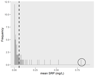
Figure A1 Distribution of mean SRP concentrations (mg L⁻¹) during late-summer low-flow conditions for 128 gauged watersheds with more than three SRP samples collected during late-summer low flows. Note that one outlier (circled value) was excluded prior to model development. The dashed line indicates the mean of all mean SRP values.

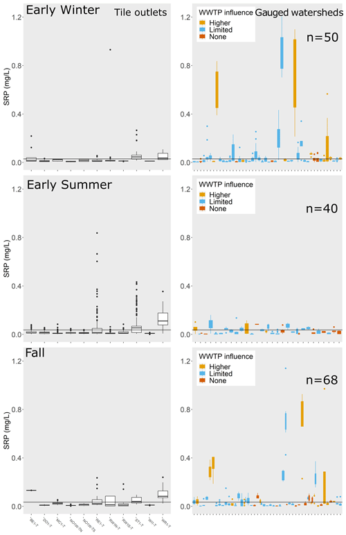
Figure A2 SRP concentrations (mg L⁻¹) for tile outlets and during low-flow conditions for gauged watersheds for early winter, early summer, and fall. See main text for similar plots for other seasons. The horizontal line in each plot is the mean SRP concentration among tile outlets for that season. The number of gauges for which low-flow data were available in each season is printed on the plot. For gauged watersheds, the color of the boxplots indicates the degree of influence from wastewater treatment plants: orange indicates wastewater treatment plant density > 0.005 sites km⁻², blue indicates wastewater treatment plant density < 0.005 sites km⁻² but greater than zero, and red indicates no wastewater treatment plant sites in the watershed. To improve data visibility, the y axis for SRP was limited to a maximum of 1.25 mg L⁻¹, which eliminated a small number of outliers from the plots for tile outlets (n= 34 out of 11 079 low-flow records) and gauged watersheds (n= 16 out of 2696 low-flow records).

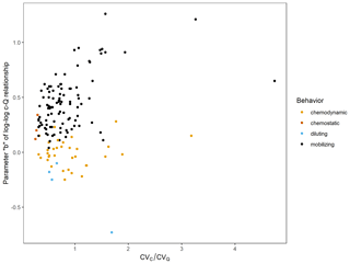
Figure A3 Parameter b (slope) of the event-scale log–log C–Q relationship for soluble reactive phosphorus (SRP, mg L⁻¹) in relation to ${\mathrm{CV}}_C/{\mathrm{CV}}_Q$ for 143 gauged watersheds. Color indicates export behavior based on criteria defined for b and ${\mathrm{CV}}_C/{\mathrm{CV}}_Q$. Chemostatic: ${\mathrm{CV}}_C/{\mathrm{CV}}_Q$ ≦ 0.3 (sensu Thompson et al., 2011); chemodynamic: ${\mathrm{CV}}_C/{\mathrm{CV}}_Q$ > 0.3 and no significant b (p>0.05); diluting: significant b<0; mobilizing: significant b>0.

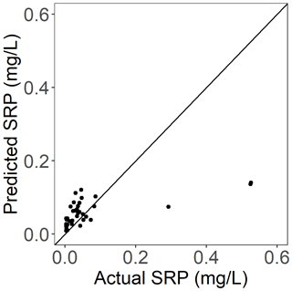
Figure A4 Actual vs. predicted late-summer SRP concentrations (mg L⁻¹) for gauged streams and rivers in the independent test dataset (i.e., not used to build the model). R²= 0.41, RMSE = 0.010, p<0.0001. Solid line shows 1-to-1 relationship.

Table A1 Linear regression statistics for mean SRP (log scale) during low-flow conditions in relation to the density of wastewater treatment plants (sites km⁻²) across gauged watersheds by season. Linear regressions were calculated for all sites and were recalculated where sites with a density of wastewater treatment plants > 0.005 sites km⁻² were excluded. Note that “WWTP” refers to wastewater treatment plant throughout.

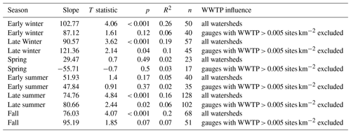
Table A2 Linear regression statistics for mean SRP (log scale) during low-flow conditions in relation to percentage crop cover across gauged watersheds by season. Linear regressions were calculated for all sites and were recalculated for sites with no wastewater treatment plant influence in their watersheds.

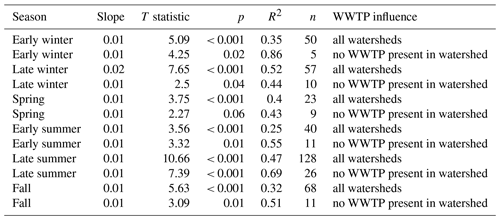
Table A3 Mean SRP during low-flow conditions (flow conditions ≦ lowest 25th percentile of flows on record) for each gauged watershed during each season. Note that means were only calculated where gauged watersheds had ≧ three low-flow samples collected during a season. NA indicates that fewer than three low-flow samples were collected during that season. “WS area” refers to the watershed land area draining into each gauge (in km²). “WWTP density” is wastewater treatment plant density for each watershed (in sites km⁻²).

Table A4 Number of SRP samples collected during low-flow conditions in each season for each gauged watershed. Note that mean SRP values (Table S3) were only calculated in seasons where fewer than three samples had been collected during low-flow conditions for that gauged watershed.

Table A5 Linear regression statistics for the log–log relationship between SRP concentrations (mg L⁻¹) and normalized flow ($Q/Q_{\mathrm{GM}}$). The regressions were run twice. The first regressions (denoted with (1) in the table) included all samples collected for a given site. The second set of regressions (denoted with (2) in the table) excluded samples collected during late-summer low flows. “Percentage change in slope” indicates the change in slope between the first and second regression for each site. CV${}_C/{\mathrm{CV}}_Q$ is reported using all samples collected for each site. Statistics in bold indicate statistically significant (p<0.05) relationships.

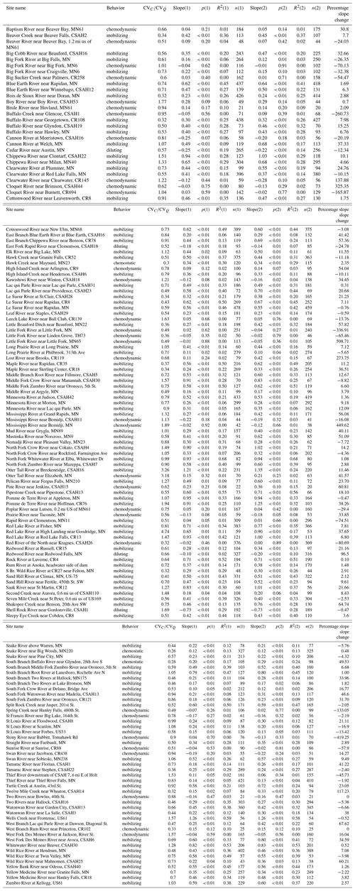
Table A6 Conditional permutation importance value for predictor variables used in the random forest model. Note that AOI refers to the area of interest and defines whether variables were summarized at the watershed (Ws) or catchment (Cat) scale as well as whether they were limited to the 100 m riparian areas in the watershed or catchment (Rp100).