An intercomparison of four gridded precipitation products over Europe using an extension of the three-cornered-hat method

Precipitation is arguably one of the most relevant surface variables impacting human lives on the planet, but global-coverage, high-resolution and good-quality observations are not readily available. In particular, gridded observational datasets are much needed for model development and forecast quality assessment. Here, we compare the quality of four types of gridded precipitation products over Europe, namely a rain gauge interpolation, a satellite-derived product, a radar composite and a reanalysis. Each product has its own strengths and weaknesses, and since each precipitation estimate uses different measuring techniques, we can employ a triangulation method to estimate the error variance of each product with respect to the unknown true values. Results show that (a) the satellite product has limited quality over Europe and may be problematic to use in quantitative forecast evaluation and diagnostics; (b) the radar composite has spurious features that need to be considered when used in verification; (c) all products struggle in topographically complex areas; (d) the rain gauge interpolation is not free of errors, despite rain gauges often being treated as ground truth in the literature; and (e) the reanalysis dataset produces, in some cases, the best available estimates, particularly over the European near-coastal waters.

1 Introduction

Surface precipitation affects many aspects of human life on Earth: rain, droughts and floods can threaten human lives and infrastructures and can impact agriculture and energy production, biodiversity, forest fires, air quality, availability of drinking water, health, businesses, and everyday lives. Unsurprisingly, precipitation forecasts are an essential part of weather prediction, and the importance of measuring precipitation globally has been widely recognised (Hou et al., 2014). In particular, gridded precipitation observations are needed to assess the socio-economic impacts of precipitation hazards, to better understand physical processes, to calibrate numerical models or to verify weather forecasts.

While, nowadays, many observational precipitation products are available (see, for example, Beck et al., 2019, for a list of 26 alternatives), their spatial coverage, horizontal resolution, temporal sampling and overall quality vary widely. Each product has its own strengths and weaknesses: for instance, some products have very good quality but are only available over land or for certain countries; other datasets have global coverage at the cost of lower resolution; some datasets include rain estimates over the oceans, where in situ observations are not available; and some products are designed to be available in near-real time, while other products put more emphasis on quality control and homogeneity.

In view of this variety of products, it is crucial to assess both their uncertainty and their suitability for specific purposes. This study was guided by the need to verify kilometre-scale global forecasts produced under the framework of the Destination Earth programme (Hoffmann et al., 2023). In the case of forecast verification, the quality of the observational datasets affects the score results and can potentially alter the conclusions reached (Bowler, 2008; Candille and Talagrand, 2008; Duc and Saito, 2018; Bessac and Naveau, 2021; Ramon et al., 2023). In practical terms, high-resolution observations with a wide coverage over land and oceans should be preferred for the verification of global kilometre-scale forecasts. Precipitation is highly variable in both space and time, and its highly skewed distribution renders time or space aggregates non-representative of the most extreme conditions occurring within a grid box.

In this work, we compare the quality of four independently derived precipitation products over Europe (see Sect. 3.1). We employ a triangulation technique to estimate the error variance of each product (described in Sect. 3.3). This method relies on the assumption that the precipitation estimates are made using independent observation and retrieval techniques. Here, we have extended the method to allow for a certain degree of inter-dependence in the datasets. Therefore, we review the existing measurement techniques in Sect. 2 to understand their strengths and shortcomings. Results and conclusions follow in Sects. 4 and 5.

2 Four alternative ways of estimating precipitation

Several measurement techniques are available to estimate surface precipitation (Prigent, 2010; Sun et al., 2018). Rain gauges are the most direct way of obtaining observations, and, if well maintained and installed, they produce good-quality records. However, gauges experience problems measuring when there are high winds or when the precipitation is not in the liquid phase, and they produce estimates that are only valid at the local scale. Moreover, their installation and maintenance are costly, and there is, therefore, a limited number of such stations, mostly concentrated around populated areas. Gridded products can be produced from gauge networks, and their quality will be dictated by the number of stations within each grid cell.

Remote sensing provides an alternative to in situ measurements of surface precipitation. Weather radars can measure precipitation in the surroundings by sending out horizontal beams of electromagnetic waves and measuring the energy reflected by water suspended in the air. Several types of radars with different frequency bands are operating in many countries. Radars produce high-resolution information down to the kilometre scale, but they have known issues: beam attenuation (quality degrades when moving away from the radar location); beam blocking by topography; the indirect nature of the measurements, which introduces errors when transforming measured reflectivity to precipitation rates (Z–R relationship); spurious echoes and clutter due to wind turbines, bird migrations, planes, etc.; or the inability to measure close to ground level, therefore confusing virga for precipitation or missing low-level precipitation. Weather radars are also a costly infrastructure, and they are only available for populated areas and in countries that can afford it. Gridded products can be made by combining information from multiple radars.

Satellite-mounted remote sensing devices allow the measurement of precipitation from space in regions where traditional observations or weather radars are not available, e.g. over the oceans or in remote areas. Many types of satellites and instruments can be employed. Infrared imagers on geostationary satellites can estimate convective precipitation through brightness temperatures and cloud top height information. Low-Earth-orbiting satellites can also estimate precipitation by measuring passive microwave radiation or by employing active microwave instruments (e.g. on-board weather radars). The main sources of uncertainty for satellite-derived precipitation observations are the indirect nature of the observations; the sparse or intermittent coverage of polar-orbiting satellites; the inhomogeneity of the techniques employed over land and sea, e.g. passive microwave imagers; the difficulties in detecting warm-cloud (low-level) precipitation; and the algorithms needed to combine the available information from multiple instruments and satellites.

Finally, reanalyses combine numerical weather prediction models and data assimilation techniques to estimate a gap-free and physically consistent state of the atmosphere. Current global reanalyses have coarser resolutions than other state-of-the-art precipitation observation systems, but they offer an additional perspective with regard to surface precipitation. Precipitation estimates from reanalyses are not derived directly from precipitation measurements but rather by means of observations of other atmospheric quantities such as temperature, humidity or atmospheric circulation, which, in turn, shape precipitation in the model. Precipitation estimates from reanalyses inherit the weaknesses of the models employed (e.g. they rely on parameterisations) and have difficulties in representing small-scale convective precipitation but can do a good job reproducing larger-scale stratiform precipitation.

3 Data and methods

3.1 Datasets

Four gridded datasets covering Europe have been employed. Table 1 summarises the main characteristics of each of them. While many other gridded precipitation datasets are available, for this study, we have selected one product for each type of measurement technique to guarantee the independence of products as much as possible.

Table 1 Main characteristics of the observational datasets employed.

* Fewer instruments available above 60° N.

3.1.1 E-OBS

E-OBS (Cornes et al., 2018) is a gridded product produced by KNMI and derived from in situ rain gauge measurements over Europe. As such, it only provides values over land. The station density within each grid cell is variable in both space and time, impacting the quality of the precipitation estimates. We have employed version 26.0e of this dataset. As an in situ product, it is sometimes used as a reference for calibrating or verifying other types of measurements, although that is only valid in areas of high station density. Moreover, this product is not free of errors. For instance, the daily accumulation periods of some gauges do not correspond to accumulations at midnight. All our analyses are agnostic and do not assume that one product is an error-free reference used to benchmark others.

3.1.2 IMERG

The Integrated Multi-satellitE Retrievals for Global Precipitation Mission (IMERG) (Huffman et al., 2023, 2020) is a satellite-derived product combining information from passive and active sensors aboard both geostationary and polar-orbiting satellites. Its main strength is that it provides global coverage (including oceans) with a 30 min time sampling on a 0.1 ° grid. The IMERG algorithm is complex and merges infrared temperatures, passive microwave and active radar soundings. We employ the Final Run IMERG version 07B product, which has been quality-controlled and scaled so that monthly totals match those of rain gauges, where available.

3.1.3 OPERA

The Operational Program on the Exchange of Weather Radar Information (OPERA) (Huuskonen et al., 2014; Saltikoff et al., 2019) produces a weather radar composite combining information from around 200 radars from 25 European countries. This radar network is very inhomogeneous in terms of radar technologies employed in different countries (bands, scanning strategy, etc.), but the OPERA data centre (ODC, also known as Odyssey) produces the composites from the individual information of each radar, which minimises the differences due to post-processing. The hourly total precipitation composite is available on a grid of 2 km resolution every 15 min. As a very basic measure of quality control, we have set any values above 300 mm h⁻¹ as invalid.

3.1.4 ERA5

ERA5 (Hersbach et al., 2023, 2020) is a state-of-the-art global reanalysis produced by ECMWF. By employing a frozen numerical weather prediction model and data assimilation scheme, it recreates the state of the atmosphere during the past decades. A reanalysis constrains the solution to be physically consistent and close to the available existing observations. Therefore, it produces accurate estimates of precipitation even in regions without direct observations. Indeed, ERA5 does not assimilate precipitation observations other than the NCEP stage-IV precipitation over the US. This means that precipitation estimates from ERA5 in Europe are derived mainly from other atmospheric quantities constrained by observations (e.g. humidity, geopotential height, winds) and their relationship to precipitation in the model. Total precipitation in ERA5 includes both parameterised and large-scale precipitation in the forms of rain and snow and takes into account some of the precipitation evaporation.

3.2 Data collocation

In order to perform the comparative assessment, all the data have been collocated in a common space and time grid. First, the data were accumulated to daily total precipitation (00:00–00:00 UTC). Then each dataset was interpolated to a 0.1°×0.1° latitude–longitude grid. In particular, the OPERA radar data were interpolated from a finer grid using a conservative interpolation (in particular, the “average” method of the gdalwarp utility), and the ERA5 reanalysis was interpolated from a coarser grid with a nearest-neighbour method. The E-OBS and IMERG products were already on a 0.1° grid.

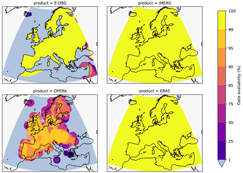
The period employed covers October 2016 to September 2021, amounting to 5 years or 1826 d. The data have been cropped to a European domain covering 30 to 70° N and 20° W to 40° E. However, some of the assessed products do not cover the whole domain, and a full comparison is only possible for those grid points where all four products are available. Figure 1 shows a map of data availability (in percent) for each product. E-OBS is only available over land. The radar composite covers only a limited number of countries with an additional offshore buffer. ERA5 and IMERG cover the whole region and for all times, although IMERG has a reduced satellite coverage above of 60° N.

Figure 1 Data availability for each product, indicated as a percentage of the whole period.

The assessment is performed separately at each grid point. To ensure that the statistics (means, variances, covariances) computed for each product are comparable, only the days that are available for all four products are considered. Therefore, the exact periods at each location can differ slightly. ERA5, IMERG and E-OBS are available almost all the time, and so the dates used at each grid point are dictated by the availability of OPERA data. Additionally, we have discarded any grid point with less than 75 % data availability, ensuring sample sizes of at least 1370 d. This is within the range of 500 to 5000 samples recommended by Sjoberg et al. (2021) for the three-cornered-hat (3CH) method.

3.3 Three-cornered-hat error estimation

The three-cornered-hat (3CH) method was originally developed to estimate random errors of atomic clocks (see Sjoberg et al., 2021, for a comprehensive review of the method). The 3CH and the related triple-collocation method have been used in the areas of weather and climate to estimate observational errors of wave height (Janssen et al., 2007), sea surface temperature (O'Carroll et al., 2008), precipitation (Roebeling et al., 2012; Massari et al., 2017; Alemohammad et al., 2015), surface wind (Abdalla and De Chiara, 2017), soil moisture (Gruber et al., 2016) and radio occultation measurements (Anthes and Rieckh, 2018).

The goal is to quantify the error incurred by an observation system A when trying to estimate some (unknown) true values τ. We define the (additive) error of A as follows: ${\mathcal{E}}_A=A-\mathit{\tau }$. The method relies on decomposing the variance of the difference of two independent observation systems A and B as

$$\begin{array}{}\text{(1)}& \begin{array}{rl}\mathrm{Var}(A-B)& =\mathrm{Var}({\mathcal{E}}_A-{\mathcal{E}}_B)=\mathrm{Var}\left({\mathcal{E}}_A\right)+\mathrm{Var}\left({\mathcal{E}}_B\right)\\ & -\mathrm{2}\mathrm{Cov}({\mathcal{E}}_A,{\mathcal{E}}_B),\end{array}\end{array}$$

which can then be approximated by the sum of the error variance of each product:

$$\begin{array}{}\text{(2)}& \mathrm{Var}(A-B)\approx \mathrm{Var}\left({\mathcal{E}}_A\right)+\mathrm{Var}\left({\mathcal{E}}_B\right).\end{array}$$

The approximation is only valid if the observational errors of products A and B are uncorrelated, i.e. if the observations are derived independently. For example, the second panel in Fig. 2 shows the variance of the differences between the gauge product and the radar composite. If we assume that the radar and gauges measure the same unknown quantity τ employing different techniques, which should produce uncorrelated errors, we can interpret Fig. 2 as the sum of the individual error variances of both products. Areas with large values in Fig. 2 are caused by errors in either product A or product B or in both (notice that variances cannot be negative by definition, and so there is no room for error compensation).

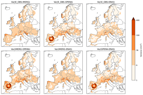
Figure 2 Variance of the differences between pairs of products. A circular pattern around Madrid can be clearly seen for all panels involving the radar composite, uncovering a clear problem in that dataset even before performing the 3CH analysis.

At this point, we cannot say what proportion of the difference variance is attributable to each product error. To that end, if we have a third independent observation system C, we can repeat the above steps with differences between A and C and B and C to obtain a linear system of three equations and six unknowns (three variances and three covariances) that can be solved to obtain a quantitative result.

$$\begin{array}{}\text{(3)}& \left\{\begin{array}{l}\mathrm{Var}(A-B)=\mathrm{Var}\left({\mathcal{E}}_A\right)+\mathrm{Var}\left({\mathcal{E}}_B\right)-\mathrm{2}\mathrm{Cov}({\mathcal{E}}_A,{\mathcal{E}}_B)\\ \mathrm{Var}(A-C)=\mathrm{Var}\left({\mathcal{E}}_A\right)+\mathrm{Var}\left({\mathcal{E}}_C\right)-\mathrm{2}\mathrm{Cov}({\mathcal{E}}_A,{\mathcal{E}}_C)\\ \mathrm{Var}(B-C)=\mathrm{Var}\left({\mathcal{E}}_B\right)+\mathrm{Var}\left({\mathcal{E}}_C\right)-\mathrm{2}\mathrm{Cov}({\mathcal{E}}_B,{\mathcal{E}}_C)\end{array}\right.\end{array}$$

Assuming that the three error covariance terms are small and can be neglected, the system of equations can be solved for the error variances from the three collocated datasets.

$$\begin{array}{}\text{(4)}& \left\{\begin{array}{l}\mathrm{Var}(A-B)=\mathrm{Var}\left({\mathcal{E}}_A\right)+\mathrm{Var}\left({\mathcal{E}}_B\right)\\ \mathrm{Var}(A-C)=\mathrm{Var}\left({\mathcal{E}}_A\right)+\mathrm{Var}\left({\mathcal{E}}_C\right)\\ \mathrm{Var}(B-C)=\mathrm{Var}\left({\mathcal{E}}_B\right)+\mathrm{Var}\left({\mathcal{E}}_C\right)\end{array}\right.\end{array}$$

3.4 Four-cornered-hat error estimation

In our case, we have identified four observational systems; therefore, we can constrain the computation a bit more. In the general case of N datasets, there are $\left(\genfrac{}{}{0ex}{}{N}{\mathrm{2}}\right)$ unique pairs of products for which we can write an equation like Eq. (1). The resulting system of linear equations is under-determined, with $\left(\genfrac{}{}{0ex}{}{N}{\mathrm{2}}\right)$ equations, N unknown variances and $\left(\genfrac{}{}{0ex}{}{N}{\mathrm{2}}\right)$ unknown covariances. For N=4, we have six equations and 10 unknowns.

$$\begin{array}{}\text{(5)}& \left\{\begin{array}{l}\mathrm{Var}(A-B)=\mathrm{Var}\left({\mathcal{E}}_A\right)+\mathrm{Var}\left({\mathcal{E}}_B\right)-\mathrm{2}\mathrm{Cov}({\mathcal{E}}_A,{\mathcal{E}}_B)\\ \mathrm{Var}(A-C)=\mathrm{Var}\left({\mathcal{E}}_A\right)+\mathrm{Var}\left({\mathcal{E}}_C\right)-\mathrm{2}\mathrm{Cov}({\mathcal{E}}_A,{\mathcal{E}}_C)\\ \mathrm{Var}(A-D)=\mathrm{Var}\left({\mathcal{E}}_A\right)+\mathrm{Var}\left({\mathcal{E}}_D\right)-\mathrm{2}\mathrm{Cov}({\mathcal{E}}_A,{\mathcal{E}}_D)\\ \mathrm{Var}(B-C)=\mathrm{Var}\left({\mathcal{E}}_B\right)+\mathrm{Var}\left({\mathcal{E}}_C\right)-\mathrm{2}\mathrm{Cov}({\mathcal{E}}_B,{\mathcal{E}}_C)\\ \mathrm{Var}(B-D)=\mathrm{Var}\left({\mathcal{E}}_B\right)+\mathrm{Var}\left({\mathcal{E}}_D\right)-\mathrm{2}\mathrm{Cov}({\mathcal{E}}_B,{\mathcal{E}}_D)\\ \mathrm{Var}(C-D)=\mathrm{Var}\left({\mathcal{E}}_C\right)+\mathrm{Var}\left({\mathcal{E}}_D\right)-\mathrm{2}\mathrm{Cov}({\mathcal{E}}_C,{\mathcal{E}}_D)\end{array}\right.\end{array}$$

In order to find a unique solution, we need N additional constraints. For the 3CH (N=3), all three covariance terms were set to zero. For N=4, we can set any four of the six covariance terms to zero, and then the two remaining covariance terms will be explicitly computed by the method.

Assessing which two covariance terms should be computed is a science-informed but subjective matter. Checking the independence of two observational products comes down to identifying confounding variables that could have an impact on the measurements of both measuring techniques. Notice that independently derived products do not directly guarantee uncorrelated errors. For example, if two measuring approaches are sensitive to raindrop size or if two products have difficulties in identifying low-level precipitation, this will result in correlated errors in the data. Small sample sizes can also result in non-zero covariances due to sampling randomness. In our setting, the following error orthogonality assumptions have been made:

• Satellite and gauge errors are considered to be independent since their measurement techniques are very different in nature. Although the final IMERG product is bias-adjusted with the monthly total precipitation of some gauge stations, the variability of daily total values is only weakly affected by that adjustment. Therefore, we set $\mathrm{Cov}({\mathcal{E}}_{\mathrm{IMERG}},{\mathcal{E}}_{\mathrm{EOBS}})=\mathrm{0}$.

• Radar and gauge errors are considered to be independent since their measurement techniques are very different in nature. OPERA does not use rain gauges to calibrate the composites. Therefore, we set $\mathrm{Cov}({\mathcal{E}}_{\mathrm{OPERA}},{\mathcal{E}}_{\mathrm{EOBS}})=\mathrm{0}$.

• ERA5 and gauge errors are considered to be independent since ERA5 does not assimilate any rain gauge information beyond the US. Therefore, we set $\mathrm{Cov}({\mathcal{E}}_{\mathrm{ERA}\mathrm{5}},{\mathcal{E}}_{\mathrm{EOBS}})=\mathrm{0}$.

• ERA5 and radar errors are independent since ERA5 does not assimilate any radar data over Europe. Therefore, we set $\mathrm{Cov}({\mathcal{E}}_{\mathrm{ERA}\mathrm{5}},{\mathcal{E}}_{\mathrm{OPERA}})=\mathrm{0}$.

• ERA5 assimilates radiances from many satellites, including microwave imagers, microwave sounders and infrared imagers (see Fig. 5 in Hersbach et al., 2020). Some of those instruments (e.g. the GPM microwave imagers) are also used by the IMERG algorithm (Huffman et al., 2020). Therefore, we have decided to explicitly compute Cov(ℰ_IMERG,ℰ_ERA5).

• Some GPM satellites used in IMERG incorporate a dual-band weather radar on board. Although the overall characteristics of these on-board radars are very different from conventional ground-based radars, some aspects, such as the equations employed to convert radar reflectivity to precipitation rates, are common to both estimate techniques. Therefore, we have decided to explicitly compute Cov(ℰ_IMERG,ℰ_OPERA).

Some extensions of the 3CH that take advantage of more than three collocated datasets have already been proposed in the literature. On the one hand, Sjoberg et al. (2021) already showed how N datasets can be used to obtain $\left(\genfrac{}{}{0ex}{}{N-\mathrm{1}}{\mathrm{2}}\right)$ different estimates of Var(ℰ) for each product by selecting distinct triplets of datasets and employing the 3CH for each subset. Alternatively, Pan et al. (2015) present the equations of the 3CH (albeit referring to triple collocation) assuming uncorrelated errors for all pairs of products. This turns the problem into an over-determined system which is then solved by ordinary least squares. Finally, Zwieback et al. (2012) and Vogelzang and Stoffelen (2021) present a quadruple-collocation solution which is conceptually identical to ours but based on the triple-collocation equations, which rely on slightly different assumptions. The strength of the approach we present is that the error orthogonality assumptions are underpinned by domain knowledge, resulting in a better approximation of the Var(ℰ) values (Zwieback et al., 2012).

4 Results

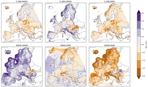
As a first step to intercompare the four datasets, the difference in the daily total mean precipitation is presented in Fig. 3 for each pair of products. The largest differences can be seen over the ocean, where OPERA is drier than IMERG and ERA5 by 2 to 5 mm and where IMERG is wetter than ERA5 by 1 to 2 mm. Over land, ERA5 and IMERG have better agreement, with important differences concentrated over high mountain ranges only. Both products are wetter than E-OBS and OPERA, although OPERA is the driest product in most locations. While these difference plots allow for the spotting of spatial patterns in the data (e.g. beam attenuation in all OPERA panels or systematic biases over Poland for E-OBS) and getting an idea of the uncertainty range, the true values are unknown; hence, we cannot judge which of the products yields a closer estimate of the true mean precipitation.

Figure 3 Mean of the differences between pairs of products.

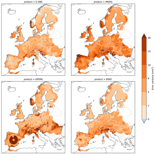
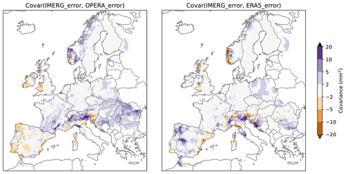
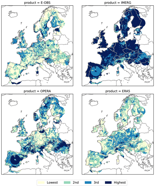
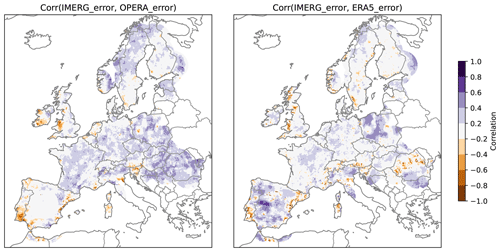
Under the assumptions made in the previous section, the 4CH method allows for an estimation of the error variances of each product and therefore ranking of the products from highest to lowest. Figure 4 shows the 4CH error variances of each product (only available over the grid points covered by all four products). The IMERG product shows the largest errors overall, which tend to be highest in coastal areas of the Iberian Peninsula and the British Isles and around the Alps. The OPERA composite also has very high error variances in some regions, clearly related to issues in particular radars, e.g. the radars in Madrid or Copenhagen; however, in other areas such as Germany, the quality is very good. Clutter can also be seen in some areas of eastern Europe. It is reassuring to see that the method can recreate the spatial error patterns produced by the radars without any knowledge of the radar locations. The E-OBS product emerges as a good product in almost all of the continents, although it has some quality issues in areas such as the Balkans. The ERA5 dataset, despite being a lower-resolution product, shows errors close to those of E-OBS and even lower errors in some regions such as Brittany or the British Isles (see Fig. A1 in the Appendix for a plot of the ranking of each product at each grid point). ERA5 has less quality in mountainous areas such as the Alps. Some localised spots in Fig. 4 have negative variance values. Those can mainly be seen for E-OBS over the Iberian Peninsula and in the northeast of Italy, with a mean value close to −1.6 mm² over those locations. Those values are unphysical since error variances must be positive by definition and result from the assumptions made in Sect. 3 not being entirely correct in those grid points (see Sect. 4e in Sjoberg et al., 2021, and Sect. 2.5 in Pan et al., 2015, for detailed discussions of when that occurs). Indeed, the error covariance between IMERG and ERA5 has strong positive values in those regions (see Fig. 5), which are then subtracted during the computation of the variance estimate of E-OBS (see Eq. 3a in Sjoberg et al., 2021). While some authors have proposed ways forward to constrain the 3CH solutions to keep them positive-definite (see, for example, Premoli and Tavella, 1993), we have not explored this avenue because the issue is minor and restricted to few locations in our case. The corresponding error correlations (see Fig. A2) are mostly positive and not particularly small, especially for the two remote sensing products.

Figure 4 The 4CH-derived error variances for the four products.

Figure 5 The 4CH-derived error covariances for the two explicitly computed pairs of products.

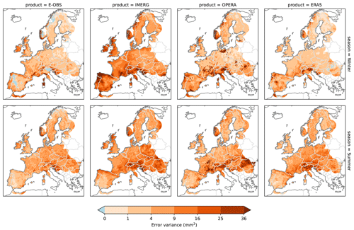
Since convective and stratiform types of precipitation have very different characteristics in terms of spatial patterns, intensity, duration or height in the atmosphere, it is reasonable to ask if the four products studied here represent these two distinct types of precipitation well. To answer that, we have stratified the results into two seasons, an extended winter (NDJFM, predominantly stratiform precipitation) and an extended summer (MJJAS, mostly convective precipitation). The results in Fig. 6 show that E-OBS, OPERA and ERA5 have better accuracy in winter than in summer, whereas IMERG has better performance in summer than in winter. This confirms that IMERG is better at sensing convective precipitation events than stratiform precipitation, whereas the opposite can be said for the other products. Still, IMERG is not better than the other three products in summer. An interesting aspect to notice in Fig. 6 is that the quality issues we saw in Fig. 4 for OPERA almost disappeared in the winter–summer stratifications. A plausible explanation is that some outliers that are only present in some days of April or October (therefore excluded in both composites) had a strong influence on the overall result (see Sect. 4 of Sjoberg et al., 2021).

Figure 6 The 4CH error variances in winter (top row) and summer (bottom row) for each observational product.

5 Conclusions

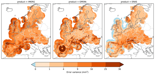
The choice of a verification dataset for global and high-resolution precipitation forecasts is challenging. From a technical perspective, IMERG is a good choice because it covers the oceans, and it produces a relatively high-resolution and mostly gap-free dataset. However, we have seen that its quality over Europe is not particularly good compared to existing alternatives. Moreover, its quality over the ocean is also not good (see Fig. A3). Both E-OBS and the OPERA radar composites provide a better alternative over European land. The OPERA data constitute a higher-resolution product, and although it might be biased with respect to in situ measurements, with a bit of additional quality controlling, it might be the best way to go about verifying high-resolution simulations over Europe. Both products have the limitation of not providing information over the oceans, which might be a problem when it comes to obtaining robust results (given that oceans cover two-thirds of our planet) or applying spatial verification techniques that rely on neighbourhood analyses. The only remaining alternative might then be using modelled products such as ERA5. Our results show that the quality of ERA5 is not far from that of E-OBS in Europe, especially in winter (in agreement with Lavers et al., 2022). However, since ERA5 is produced with a specific version of the IFS model, comparing IFS forecasts to ERA5 does not provide a very stringent evaluation as forecasting and analysis share very similar model limitations and systematic biases. Higher-resolution modelled datasets such as regional reanalyses could provide better results than ERA5, but we have not explored this option here. In short, the promise of a global-coverage, high-resolution and good-quality precipitation dataset measured from space is not yet fully realised, and, therefore, verifying global precipitation forecasts against reanalysis datasets is still a justified alternative. All the conclusions above are based on estimates of error variance obtained with an extension of the three-cornered-hat method, which, in turn, relies on a set of error covariance assumptions. Those assumptions were carefully selected based on physical considerations of the different observational systems but have not been independently validated. The error variance estimates can differ from the true error variances whenever the error orthogonality assumptions are not fulfilled.

Extending this study to other regions would be interesting. Specifically, the IMERG dataset is thought to be of better quality in the tropics due to the predominance of convective precipitation, and it has already been used there to assess the quality of convective-permitting simulations (Becker et al., 2021). Unfortunately, an analysis such as the one we presented here is only possible in areas with a good radar and gauge network. The US would be an ideal place to apply the 4CH method, but, unfortunately, there, the ERA5 assimilates the stage-IV (radar and gauges) product, making our assumptions invalid.

This study has only dealt with error variances and therefore does not directly address quality aspects of the precipitation products that might be relevant for extreme events, such as performance under heavy rain (see, for example, Sun et al., 2018). Additional analyses showing other quality aspects of the IMERG dataset in Europe can be found in Navarro et al. (2019) or O et al. (2017), whereas the quality of IMERG over the US has also been studied in Beck et al. (2019). These studies take one reference dataset as the true values and evaluate other products. However, our agnostic analysis has confirmed that gauge-based products are not free of errors either.

Appendix A

This appendix contains three additional figures. Figure A1 shows a ranking of the four products according to the 4CH analysis from the lowest to highest error variance at each grid point, which helps in realising which datasets are more accurate overall. Figure A2 displays the error correlations derived from the error covariances and variances in Figs. 4 and 5. It is worth mentioning that there is no formal guarantee that these derived correlations remain in the [−1, 1] range, and even they cannot be computed when variances are zero or negative. Finally, Fig. A3 shows an additional 3CH analysis including only IMERG, OPERA and ERA5. In this case, the errors are assumed to be uncorrelated. We can see that the IMERG and OPERA datasets struggle to represent precipitation over the oceans, whereas ERA5 has negative values there. This indicates that IMERG and OPERA errors are indeed correlated over the ocean. The results over land are comparable to those in Fig. 4, although the errors for IMERG seem to be a bit lower with this simpler hypothesis.

Figure A1 Ranking of the four products according to the 4CH error variance.

Figure A2 The 4CH-derived error correlations for the two explicitly computed pairs of products.

Figure A3 Error variance of the three products that cover the near-coastal European waters under the assumption of uncorrelated errors.