Karst aquifer discharge response to rainfall interpreted as anomalous transport

The discharge measured in karst springs is known to exhibit distinctive long tails during recession times following distinct short-duration discharge peaks. The long-tailed behavior is generally attributed to the occurrence of tortuous, ramified flow paths that develop in the underground structure of karst systems. Modeling the discharge behavior poses unique difficulties because of the poorly delineated flow path geometry and generally scarce information on the hydraulic properties of catchment-scale systems. In a different context, modeling of long-tailed behavior has been addressed in studies of chemical transport. Here, an adaptation of a continuous time random walk–particle tracking (CTRW-PT) framework for anomalous transport is proposed, which offers a robust means to quantify long-tailed breakthrough curves that often arise during the transport of chemical species under various flow scenarios. A theoretical analogy is first established between partially water-saturated karst flow, characterized by temporally varying water storage, and chemical transport involving the accumulation and release of a chemical tracer. This analogy is then used to develop and implement a CTRW-PT model. Application of this numerical model to the examination of 3 years of summer rainfall and discharge data from a karst aquifer system – the Disnergschroef high-alpine site in the Austrian Alps – is shown to yield robust fits between modeled and measured discharge values. In particular, the analysis underscores the predominance of slow diffusive flow over rapid conduit flow. The study affirms the analogy between partially saturated karst flow and chemical transport, exemplifying the compatibility of the CTRW-PT model for this purpose. Within the specific context of the Disnergschroef karst system, these findings highlight the predominance of slow diffusive flow over rapid conduit flow. The agreement between measured and simulated data supports the proposed analogy between partially saturated karst flow and chemical transport; it also highlights the potential ability of the anomalous transport framework to further enhance modeling of flow and transport in karst systems.

1 Introduction

Aquifers consist of various geological formations through which water can flow and carry chemical species. The abundance of structural heterogeneities, ranging from intricate grain arrangements at the pore scale to larger geologic structures and discontinuities at the meso- and macroscopic scales, introduces irregular and tortuous flow paths that cannot be delineated without a full physical description of the system. Achieving an accurate representation of flow and transport therefore becomes increasingly difficult with an increase in the scale and complexity of the groundwater system.

Karst systems, in particular, are known as structurally complex aquifers. They are composed of many interconnected conduits, fractures, and voids formed through the dissolution of soluble rocks, like limestone, dolostone, and gypsum, leading to the occurrence of multiple and ramified flow paths (Bakalowicz, 2005). Karst terrains are usually described, in a vertical cross section, by distinct hydrological layers whose structure affect the response of the system to incoming precipitation: (1) the surface soil layer; (2) the interface between the soil layer and the deeper saturated zone (epikarst); and (3) the deep underground, mostly phreatic, zone (endokarst). The soil and epikarst layers, referred to collectively as the exokarst, are known to exhibit lateral flow of water above and below the ground, until water reaches fractures or conduits that allow it to flow rapidly to the endokarst. This allows for some water to infiltrate downwards, while some may remain in the vadose zone and be subjected to both percolation and evapotranspiration (Jukić and Denić-Jukić, 2009). The epikarst and endokarst layers each consist of a primary (matrix) porosity composed of all bulk pores, a secondary porosity composed of the smaller joints and fissure developed during diagenesis and/or by tectonic processes, and a tertiary porosity of large fractures and voids (conduits) created due to karstification (Ford and Williams, 2007). The different types of porosities usually exhibit distinct flow patterns: rapid flow in the conduits and slow diffusive flow in the smaller fissures and the matrix. The different karst layers may exhibit a changing role in facilitating the flow or retention of water through the system as a function of water level or recharge intensity (Hartmann et al., 2014). Furthermore, the connectivity of the different porosities often results in a fracture–cave network, which dominates the flow structures in karst systems (Zhang et al., 2022).

To date, various hydrological models have been developed specifically for karst systems, to describe the commonly observed flow and transport patterns that are specific to karst systems. In particular, distributed models rely on creating a grid of cells with different hydrological parameters (e.g., Anderson and Radić, 2022; Chen et al., 2017; Kaufmann et al., 2016), while lumped parameter models parameterize the characteristics of the system. Lumped parameter models are based on different system conceptualizations (e.g., Chen and Goldscheider, 2014; Cinkus et al., 2023b; Fleury et al., 2009; Jukić and Denić-Jukić, 2009; Mazzilli et al., 2019; Rimmer and Salingar, 2006; Tritz et al., 2011) as well as neural network approaches (e.g., Afzaal et al., 2020; Cinkus et al., 2023b; Kratzert et al., 2018; Renard and Bertrand, 2017; Wunsch et al., 2022). A common, significant feature encountered in karst systems – which is difficult to capture in models – is the interplay of rapid and slow flow; this manifests as long-tailed measurements of both discharge rates (e.g., Frank et al., 2021) and chemical tracer concentrations (e.g., Goeppert et al., 2020) observed at karst springs.

In many systems that exhibit highly variable spatial velocity distributions or temporal behaviors, measurements of long tails in arrival times may be encountered. In the context of chemical transport in porous media, long tails in the arrival time of chemical tracers have long been a subject of study. Anomalous transport, which describes chemical transport that deviates from the behavior described by the traditional advection–dispersion equation (ADE), is prevalent in many system and transport scenarios (Berkowitz et al., 2006); deviations from solutions of traditional transport equations have even been observed for nondispersive diffusion (Cortis and Knudby, 2006). It has been shown that higher subsurface heterogeneity increases the degree of anomalous transport by inducing longer-than-expected (for Fickian transport) arrival times (Edery et al., 2016, 2014). Traditional ADE-based models, which rely on averaging the physical traits of the medium into a single coefficient, do not accurately predict transport in many cases. To correctly describe long-tailed events, various modeling approaches have been developed. Among these, the continuous time random walk (CTRW) framework has emerged as a suitable solution for simulating diverse transport scenarios, including the behavior of a long-time field-scale hydrological catchment (Dentz et al., 2023). The CTRW framework accounts for anomalous transport behavior and offers a more physically realistic representation of the transport processes that are encountered in real-world groundwater systems. The framework defines waiting time and step length distributions that are applied in random walks which are continuous in time, thereby capturing the complexity of transport processes (Berkowitz et al., 2006).

In the current study, the CTRW framework, which has been developed to model anomalous chemical transport, is utilized to quantify long-tailed discharge of water flow in karst systems. In this context, data from the Disnergschroef alpine study site in Vorarlberg, Austria, are revisited (Frank et al., 2021). This high-alpine karst system has been thoroughly studied and offers a catchment with a well-defined spatial boundary. The surface of the karst system is composed mainly of bare limestone with very limited soil coverage, resulting in negligible surface runoff. The plateau is characterized by dolines and depressions, further facilitating the direct flow of water into the subsurface. The vadose zone is estimated to be several hundred meters thick (Frank et al., 2021). The known extent of its recharge basin and the corresponding single spring which serves as its outlet allow for measurements of both recharge and discharge. Previous studies (e.g., Frank et al., 2021) have identified a distinct discharge response approximately 5.5 h after a rainfall event, with variations in electrical conductivity, indicative of fresh rainfall arriving at the spring outlet, observed ∼ 8 h post-event. While existing models provided a good overall fit and illuminated the divide between epikarst-to-conduit and matrix-to-conduit flows, they were less effective with respect to matching the long tails.

Accurate modeling of water movement in these complex subsurface landscapes is crucial, as many regions rely on karst systems for drinking water (Stevanović, 2019). Here, a theoretical and practical development of the CTRW framework is proposed as an approach to simulate the intricate dynamics of water movement in karst environments.

2 Conceptual and mathematical development

The conceptual development of the CTRW framework to model water flow in karst systems is founded on a proposed ansatz, in which water flow is conceptualized as distinct “water parcels” (i.e., infinitesimal volumes of water) that travel along the available flow paths. Local volumes along the flow paths, e.g., caverns, conduits, and voids, allow for the accumulation and release of water parcels and define mobile and immobile zones for water flow. The ansatz asserts that the accumulation and release of water parcels in the various volumes in the karst system resemble the accumulation and release of “parcels” of a chemical tracer (i.e., infinitesimal volumes of tracer) over time in a porous medium. As shown in Fig. 1, a cavern acting as a storage region for water parcels is analogous to tracer parcels accumulating in an immobile (or less mobile) zone. For both cases, it should be noted that the local accumulation of water parcels or an increase in the concentration of a chemical will increase their respective fluxes in the immediate local vicinity. Under similar hydraulic conditions, both fluxes create distinctive long tails when measured over a control plane at the system outlet, which is primarily a result of the structural heterogeneity of the system.

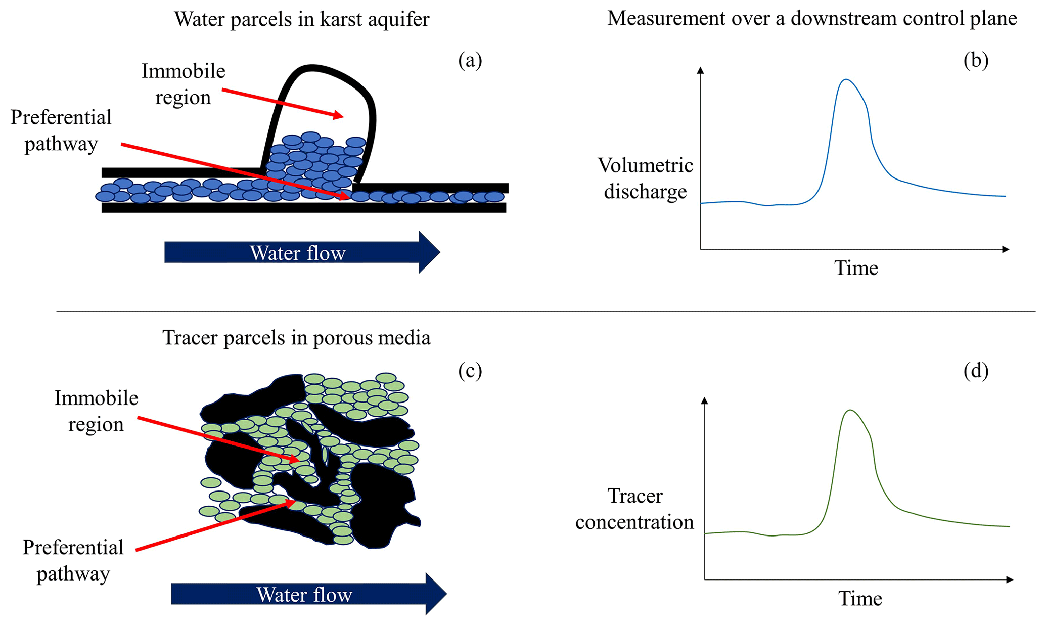
Figure 1 Schematic illustration of (a) water parcels (blue ovals) in a karst aquifer and (b) chemical tracer parcels (green ovals) in a porous medium (black grains) flowing through preferential pathways and accumulating in adjunct immobile regions. The resulting (schematic) measurements of the (c) temporal volumetric discharge and (d) tracer concentration that are measured at the spring outlet further downstream.

Characterizing the flow of water through an infinitesimal control volume can be formulated in terms of a mass balance equation that equates the net rate of fluid flow in the control volume to the time rate of change in fluid mass storage within it:

$$\begin{array}{}\text{(1)}& -{\displaystyle \frac{\partial \left(\mathit{\rho }{q}_x\right)}{\partial x}}-{\displaystyle \frac{\partial \left(\mathit{\rho }{q}_y\right)}{\partial y}}-{\displaystyle \frac{\partial \left(\mathit{\rho }{q}_z\right)}{\partial z}}={\displaystyle \frac{\partial \left(\mathit{\rho }n\right)}{\partial t}},\end{array}$$

where n is porosity; ρ is water density; and the three components of the specific discharge q are described as q_x, q_y and q_z. This equation describes the mass balance in a fully saturated domain, in which the void volume (V_v) is completely filled with water (V_w=V_v). The moisture content ($\mathit{\theta }=\frac{V_{\mathrm{w}}}{V_{\text{tot}}}$) in these cases is equal to the porosity, and the degree of saturation $({\mathit{\theta }}^{\prime }=\frac{\mathit{\theta }}{n}$) is equal to 1.

For partially saturated flow, the degree of saturation is less than 1 and the moisture content is smaller than n (as V_w < V_v). Adjusting the equation for partially saturated transient flow yields (allowing for water compressibility, to retain generality):

$$\begin{array}{}\text{(2)}& -{\displaystyle \frac{\partial \left(\mathit{\rho }{q}_x\right)}{\partial x}}-{\displaystyle \frac{\partial \left(\mathit{\rho }{q}_y\right)}{\partial y}}-{\displaystyle \frac{\partial \left(\mathit{\rho }{q}_z\right)}{\partial z}}={\displaystyle \frac{\partial \left(\mathit{\rho }{\mathit{\theta }}^{\prime }n\right)}{\partial t}}.\end{array}$$

Substituting $\mathit{\theta }={\mathit{\theta }}^{\prime }n$ then gives the following:

$$\begin{array}{}\text{(3)}& -{\displaystyle \frac{\partial \left(\mathit{\rho }{q}_x\right)}{\partial x}}-{\displaystyle \frac{\partial \left(\mathit{\rho }{q}_y\right)}{\partial y}}-{\displaystyle \frac{\partial \left(\mathit{\rho }{q}_z\right)}{\partial z}}={\displaystyle \frac{\partial \left(\mathit{\rho }\mathit{\theta }\right)}{\partial t}}.\end{array}$$

Deriving a description for the transport of a chemical tracer in a fully saturated porous medium within a similar control volume is achieved by a mass balance equation:

$$\begin{array}{}\text{(4)}& -{\displaystyle \frac{\partial F_x}{\partial x}}-{\displaystyle \frac{\partial F_y}{\partial y}}-{\displaystyle \frac{\partial F_z}{\partial z}}=n{\displaystyle \frac{\partial C}{\partial t}}.\end{array}$$

The chemical mass flux (in one direction) is defined by advection and diffusion terms:

$$\begin{array}{}\text{(5)}& F_{\mathrm{i}}=q_{\mathrm{i}}C-n{D}_{\mathrm{i}}{\displaystyle \frac{\partial C}{\partial i}}.\end{array}$$

Substituting Eq. (5) into Eq. (4) yields the following:

$$\begin{array}{}\text{(6)}& \begin{array}{rl}& {\displaystyle \frac{\partial }{\partial x}}\left(n{D}_x{\displaystyle \frac{\partial C}{\partial x}}\right)-{\displaystyle \frac{\partial }{\partial x}}\left(q_{x}C\right)+{\displaystyle \frac{\partial }{\partial y}}\left(n{D}_y{\displaystyle \frac{\partial C}{\partial y}}\right)\\ & -{\displaystyle \frac{\partial }{\partial y}}\left(q_{y}C\right)+{\displaystyle \frac{\partial }{\partial z}}\left(n{D}_z{\displaystyle \frac{\partial C}{\partial z}}\right)-{\displaystyle \frac{\partial }{\partial z}}\left(q_{z}C\right)=n{\displaystyle \frac{\partial C}{\partial t}}.\end{array}\end{array}$$

(Note that the appearance of the porosity variable, n, in the terms of Eqs. (4)–(6) is easily rearranged and that these equations can be simplified if n is assumed to be constant in space.)

By drawing the analogy in the ansatz between the dynamics of water parcels and chemical tracers and noting the similar forms of Eqs. (3) and (4), the description of the mass balance of water in a partially saturated domain is (at least) mathematically analogous to the description of the mass balance of a chemical tracer in a saturated domain. This results in the intrinsic connection of C ⇔ ρθ, both with units of mass per volume. Therefore, in a 1D direction, the analogy of the mass flux can be defined as follows: $\mathit{\rho }{q}_x\equiv n{D}_x\frac{\partial C}{\partial x}-q_{x}C$. This connection incorporates hydrodynamic dispersion, which is inherent in chemical transport resulting in observed long tails, into the description of the partially saturated water parcels moving within the conceptual karst domain. Thus, the analogy of chemical transport and water flow is expected to show long-tailed behavior in simple flow scenarios, and it has even been established for pure diffusion (Cortis and Knudby, 2006).

Thus, transport equations – either advection–dispersion equations (ADE; Eq. 7) for Fickian transport or a CTRW formulation for non-Fickian transport (see Sect. 3.1) – can be used, where the chemical tracer concentrations that these equations solve for C(x,t) are conceptually identical to the relative concentration of water parcels. The concentration at a specific point is analogous to the moisture content, and the classical C(t) breakthrough curve is analogous to the (volumetric) amount of water per unit time reaching the domain outlet (or measurement plane).

3 Methods

3.1 CTRW-PT simulations

In this study, a particle tracking (PT) implementation of the CTRW framework was employed to devise a model capable of simulating spring discharge using the rainfall data as input. The CTRW-PT model, characterized by stochastically defined particle transitions, is a Lagrangian approach to solving the partial differential equations defined in the CTRW mathematical framework. The movement of the particles, representing water parcels as described in the ansatz (see Sect. 2), is described by equations that define the probability of particles making transitions in both space and time (Elhanati et al., 2023). For 1D cases, the transport is governed by two probability density functions, p(s) and ψ(t), which define the particle movement in space and time, respectively. An exponential from for p(s) and a truncated power law (TPL) form for ψ(t) are used:

$$\begin{array}{}\text{(7)}& {\displaystyle }& {\displaystyle }p\left(s\right)={\mathit{\lambda }}_{\mathrm{s}}^{\mathrm{2}}\exp (-{\mathit{\lambda }}_{\mathrm{s}}s),\text{(8)}& {\displaystyle }& {\displaystyle }\mathit{\psi }\left(t\right)=C{\displaystyle \frac{\exp (-t/t_{\mathrm{2}})}{(\mathrm{1}+t/t_{\mathrm{1}}{)}^{\mathrm{1}+\mathit{\beta }}}}.\end{array}$$

Here, ${\mathit{\lambda }}_{\mathrm{s}}^{\mathrm{2}}$ and C serve as normalization factors for p(s) and ψ(t), respectively. The TPL is governed by β, the power law exponent (0 < β < 2), which is a measure of the non-Fickian nature of the transport; t₁, the characteristic transition time; and t₂, the cutoff time to initiate transition to Fickian transport. The particle velocity, v_ψ, and the generalized dispersion, D_ψ, are defined as the first and second spatial moments of the chemical species plume in the flow direction (Berkowitz et al., 2006) For a 1D system, this results in the following:

$$\begin{array}{}\text{(9)}& {\displaystyle }{v}_{\mathit{\psi }}={\displaystyle \frac{\stackrel{\mathrm{‾}}{s_x}}{\stackrel{\mathrm{‾}}{t}}}={\displaystyle \frac{{\int }_{\mathrm{0}}^{\mathrm{\infty }}p\left(s\right)s^{\mathrm{2}}\mathrm{d}s}{{\int }_{\mathrm{0}}^{\mathrm{\infty }}\mathit{\psi }\left(t\right)t\mathrm{d}t}},\text{(10)}& {\displaystyle }{D}_{\mathit{\psi }}={\displaystyle \frac{\mathrm{1}}{\mathrm{2}}}{\displaystyle \frac{\stackrel{\mathrm{‾}}{s_x^{\mathrm{2}}}}{\stackrel{\mathrm{‾}}{t}}}={\displaystyle \frac{\mathrm{1}}{\mathrm{2}}}{\displaystyle \frac{{\int }_{\mathrm{0}}^{\mathrm{\infty }}p\left(s\right)s^{\mathrm{3}}\mathrm{d}s}{{\int }_{\mathrm{0}}^{\mathrm{\infty }}\mathit{\psi }\left(t\right)t\mathrm{d}t}},\end{array}$$

where $\stackrel{\mathrm{‾}}{s_x}$ and $\stackrel{\mathrm{‾}}{t}$ are the mean step size and time, respectively.

Table 1 The investigated parameter space and optimized values found.

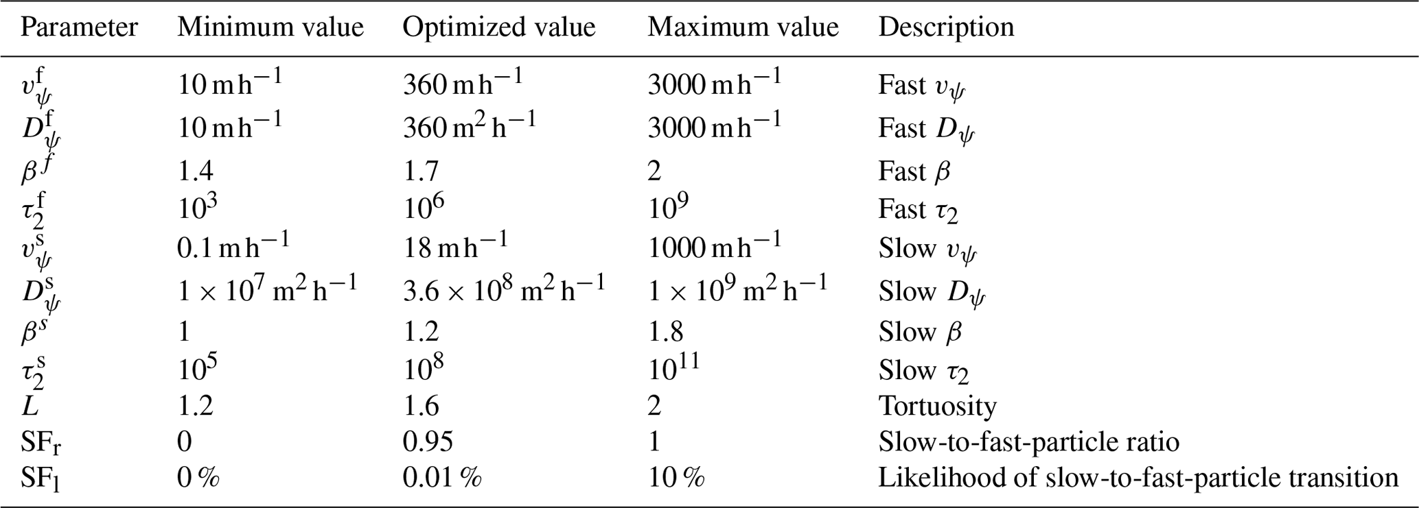
Inserting the probability density functions (Eqs. 7 and 8) into Eqs. (9) and (10) and defining ${\mathit{\tau }}_{\mathrm{2}}\equiv t_{\mathrm{2}}/t_{\mathrm{1}}$ yields a mathematical relation among v_ψ, D_ψ, β, τ₂, t₁, t₂, and λ_s (see Nissan et al., 2017, for a full mathematical development). By treating the first four variables (v_ψ, D_ψ, β, and τ₂) as fitting parameters, the other three (t₁, t₂, and λ_s) are immediately determined, allowing the optimization of the CTRW-PT model to a specific flow scenario (see Table 1).

The intricate 3D flow field of a karst system can be conceptualized in a model that considers the relationships between storage and discharge. These kinds of models, known as lumped models, have been extensively used in the simulation of karst systems (Hartmann et al., 2014). Herein, a similar approach is applied, i.e., conceptualizing the system as a series of specific physical transitions. However, in the context of the CTRW-PT model, an equivalent medium to the karst system is defined in the form of a 1D domain. Water is introduced into the domain along its entire extent and flows to the domain outlet.

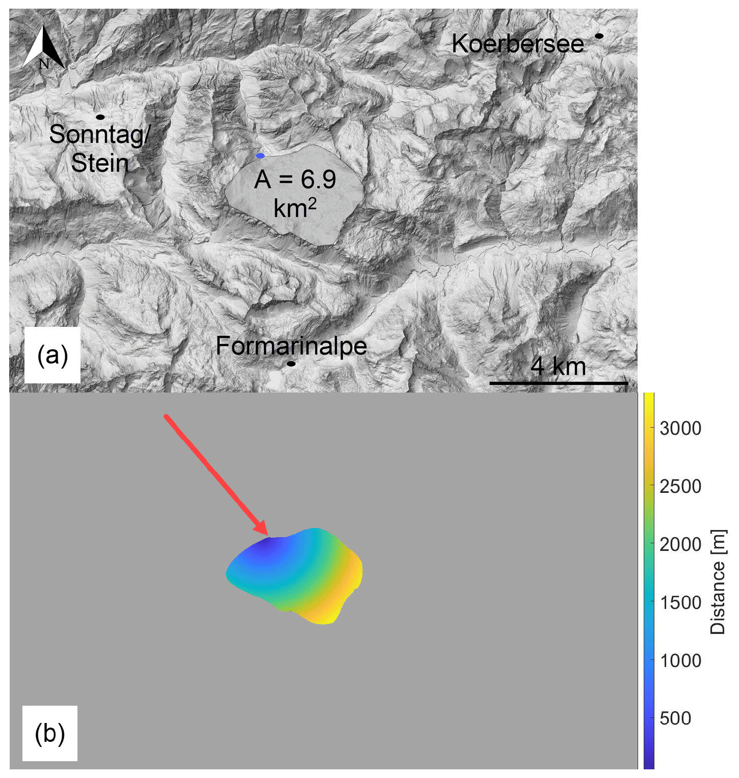
Figure 2 (a) Map of the Disnergschroef study area: the three weather stations at which rainfall was measured are marked with black dots; the measured spring outlet is marked with a blue dot (base map: Land Vorarlberg; data.vorarlberg.gv.at). (b) Distances from the catchment area to the spring outlet: the distances are marked using a color scale; the spring outlet is marked using a red arrow.

The 1D conceptualization is facilitated by the well-defined spatial characteristics of the system, namely the catchment area and spring outlet (Fig. 2a). The distance of each point on the surface of the catchment to the spring outlet is calculated (Fig. 2b), which yields a frequency histogram of distances (Fig. 3). The histogram shape is dependent upon the initial image resolution and the chosen bin size, and it yields discrete distances. To sample continuum particle entry locations without dependence on bin size, a distance distribution, fitted to the histogram using MATLAB, dictates how new particles are introduced into the system along the 1D domain (physically unrealistic, negative sampled values are set to zero). A normal distribution was chosen as a simplified representation of the distance distribution; preliminary simulation results were similar for different skewed distributions. The actual underground flow path between each point and the outlet spring is longer than the linear distance between the two points, as the water must travel through the tortuous path through the existing conduits and fissures. Therefore, the distances are multiplied by an empirical tortuosity factor (L), which serves as an optimization parameter (see Table 1).

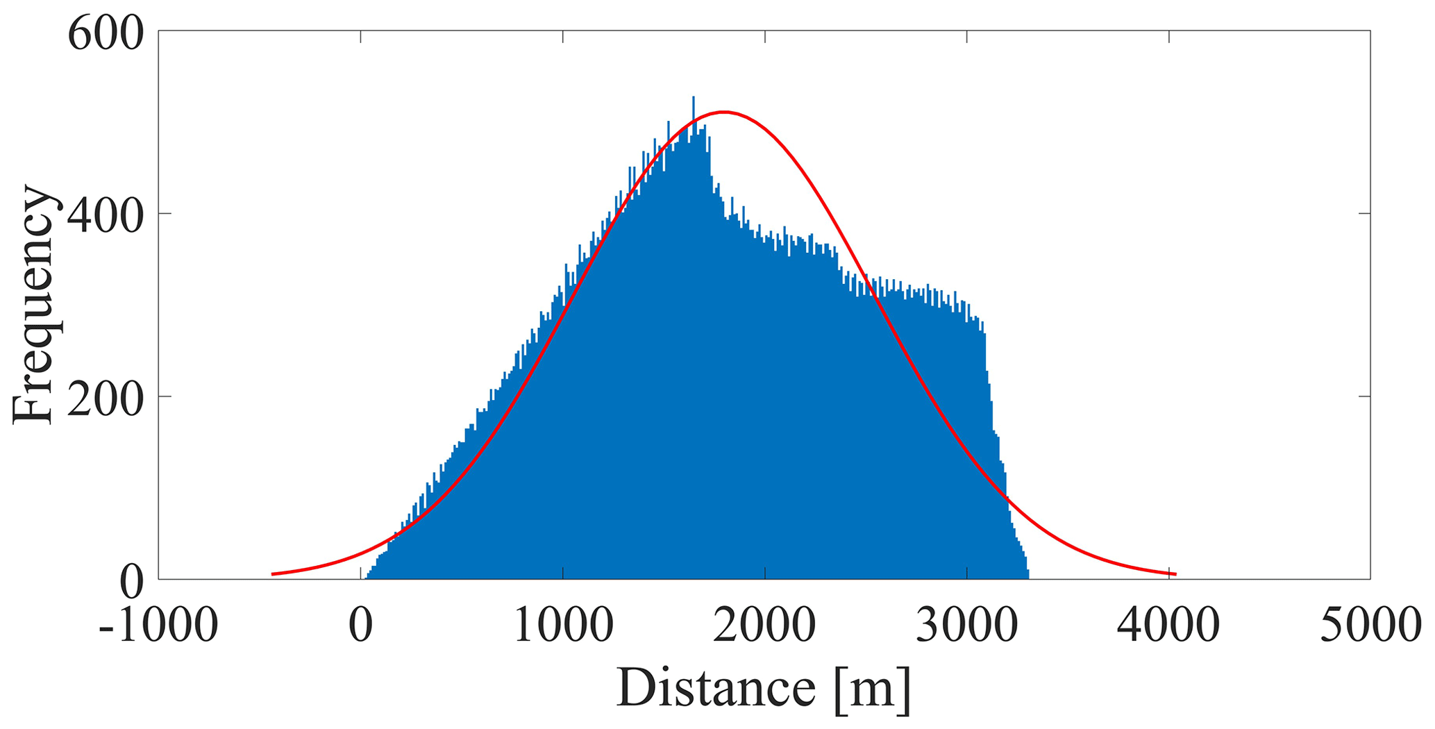
Figure 3 Distribution of distances from the catchment area to the spring outlet. The red line represents a fitted normal distribution (μ = 1.8 × 10³; σ = 747).

Discharge at the spring is sampled every 15 min (L s⁻¹). The minimum measured discharge represents the baseflow discharge. Raw rainfall data from three nearby weather stations (Fig. 2a) are measured in millimeters per 15 min. The data from the three stations are averaged, and the catchment area is used to convert the data into liters per second (Fig. 4). To achieve a higher temporal simulation resolution, linear interpolation was used to resample the time series to match a smaller simulation time step (100 s).

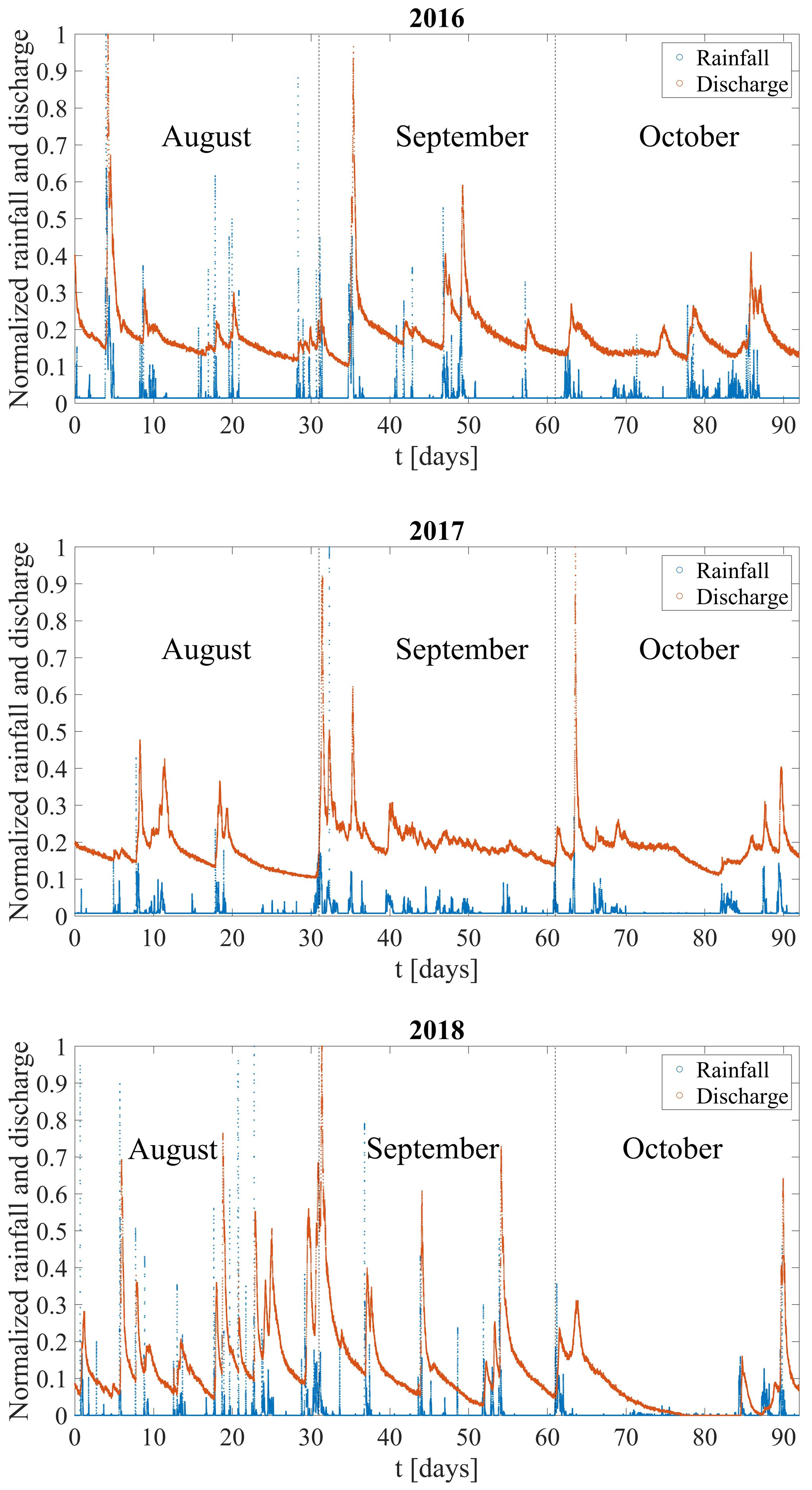
Figure 4 Rainfall and discharge curves for the 2016, 2017, and 2018 datasets. The data are normalized according to the respective maximum rainfall and discharge values for each of the 3 years.

For an ideal system, in which all incoming rainwater is discharged through the spring outlet, the ratio of total rainwater to total discharge is expected to be unity. However, considering the uncertainty in the contributions of hydraulic parameters to the catchment water budget, e.g., flow to deeper parts of the aquifer and/or other springs, and evapotranspiration, the rainfall function must be adjusted by a calculated observed recharge capacity to yield the recharge function:

$$\begin{array}{}\text{(11)}& \text{recharge}\left(t\right)=\text{rainfall}\left(t\right)\times {\displaystyle \frac{\sum \text{discharge}\left(t\right)-\text{baseflow}}{\sum \text{rainfall}\left(t\right)}},\end{array}$$

where rainfall(t) and discharge(t) are the respective measured rainfall and discharge time series. The ratio multiplying the rainfall function is defined here as the recharge capacity parameter. The baseflow was subtracted from the total discharge for the recharge capacity calculation, to account for the background discharge not related to the spring response to rainfall. While a constant recharge capacity factor is employed in this study, due to the negligible surface runoff, it is important to note that the rainfall-to-recharge ratio may be influenced by temporal variations, rainfall intensity, and spatial characteristics. Future research should consider the sensitivity of these variables for the specific scenarios considered. In cases where there is significant variability among them, other temporal and/or spatial ratios may be applied.

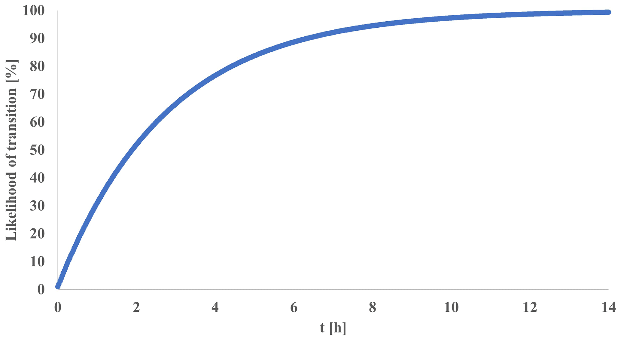
Figure 5 Likelihood of particle transition from a slow regime to a fast regime (SF_l) as a function time for SF_l = 0.01 %, representing a particle transition from slow matrix/fissure flow to fast conduit flow.

A common procedure in lumped karst models separates the flow into slow and fast components, representing the diffusive flow in the matrix and smaller fissures and the rapid flow in the conduits, respectively (Hartmann et al., 2014). The CTRW-PT, as opposed to lumped models, does not utilize water flow reservoirs; instead, it operates by tracking the motion of particles that represent water parcels. Therefore, the model was adapted to implement a similar approach: two different sets of CTRW parameters, which govern the probability density functions for particle movement (see Eqs. 7–10), are defined to represent the two flow regimes. Each particle in the simulation is defined as “slow” or “fast” and, therefore, obeys the corresponding set of CTRW parameters (see Table 1). Newly introduced particles are divided between fast and slow flow, according to a set ratio (SF_r), and they advance in space and time by their corresponding set of CTRW parameters. Furthermore, each slow particle has a likelihood to transition into a fast particle (SF_l) in each simulation iteration, by changing the set of CTRW parameters that the particle obeys. The transition from slow to fast flow illustrates the flow of water from the matrix/fissures to the conduits. While the transition of fast to slow flow is also possible in karst aquifers, i.e., when the pressure gradient allows water from the conduits to enter the matrix, the slow-to-fast transition is more prominent for this site. Thus, the likelihood of transition represents the net transition from slow to fast flow. When more particles transition back from fast to slow flow, the transition likelihood is lower. In this context, it is important to note that the CTRW-PT is a stochastic approach, in which the system parameters are represented by statistical properties. The results of CTRW-PT simulations are, therefore, representative of an ensemble average of many realizations. As depicted in Fig. 5, the likelihood of particle transition increases rapidly, with slow particles consistently transitioning into fast particles. For a transition likelihood of 0.01 % and a simulation time step of 100 s, the likelihood of a single particle making a transition surpasses 99 % after 458 steps, which amount to 45 800 s (∼ 12.7 h). In comparison, the data and simulations presented in this study span a duration of 7 951 400 s (∼ 92 d). These two parameters, governing the division of water between fast and slow flow and the transition of water from the matrix/fissures to the conduits, are pivotal in allowing the CTRW-PT model to simulate karst data.

3.2 Model optimization and comparison to field measurements

Each particle represents a volume of water. The volume per particle was calculated by dividing the total observed rainfall volume by the number of simulation particles. This enables a comparison between simulated and observed recharge by volume. Given the presence of multiple model parameters, optimization is achieved by applying a bound constraint version of the MATLAB fminsearch function (D'Errico, 2024) to minimize the root-mean-square error (RMSE) between observed and simulated discharge. A broad range of constrained parameters were investigated, as detailed in Table 1. The 2016 dataset was first used for model parameter estimation, while the 2017 and 2018 datasets served as targets for validation, by considering them for prediction using the optimized parameters from the 2016 dataset.

The Nash–Sutcliffe efficiency (NSE) and modified balance error (BE) were calculated for the optimized simulations, as a measure of the goodness of fit. The NSE and BE are the performance criteria utilized, for example, by the widely used KarstMod software (Frank et al., 2021). They are defined as the normalized variant of the mean-squared error and the relative bias of the simulated and observed flow durations, respectively:

$$\begin{array}{}\text{(12)}& {\displaystyle }& {\displaystyle }\text{NSE}=\mathrm{1}-{\displaystyle \frac{\sum \left(x_{\mathrm{s}}\right(t)-x_{\mathrm{o}}(t){)}^{\mathrm{2}}}{\sum \left(x_{\mathrm{o}}\right(t)-{\mathit{\mu }}_{\mathrm{o}}{)}^{\mathrm{2}}}},\text{(13)}& {\displaystyle }& {\displaystyle }\text{BE}=\mathrm{1}-\left|{\displaystyle \frac{\sum \left(x_{\mathrm{o}}\right(t)-x_{\mathrm{s}}(t\left)\right)}{\sum x_{\mathrm{o}}\left(t\right)}}\right|.\end{array}$$

Here, x_s is the simulated discharge, x_o is the observed discharge, and μ_o is the observed mean. The NSE performance criterion is widely used in hydrological studies and does not induce counterbalancing errors. However, it should be noted that the NSE has limitations when there is large variability in the data, and other performance criteria may be more relevant for different datasets in some cases (see Cinkus et al., 2023a, for a comparison of different performance criteria).

4 Results and discussion

4.1 Optimized simulations of measured discharge

The optimized simulation for the 2016 dataset yields a fit (Fig. 6) that captures both the rapid response of the spring discharge to rainfall events and the protracted relaxation times characterized by the long tails evident after rainfall events. The optimized model parameters for the slow diffusive and fast conduit flow components are detailed in Table 1.

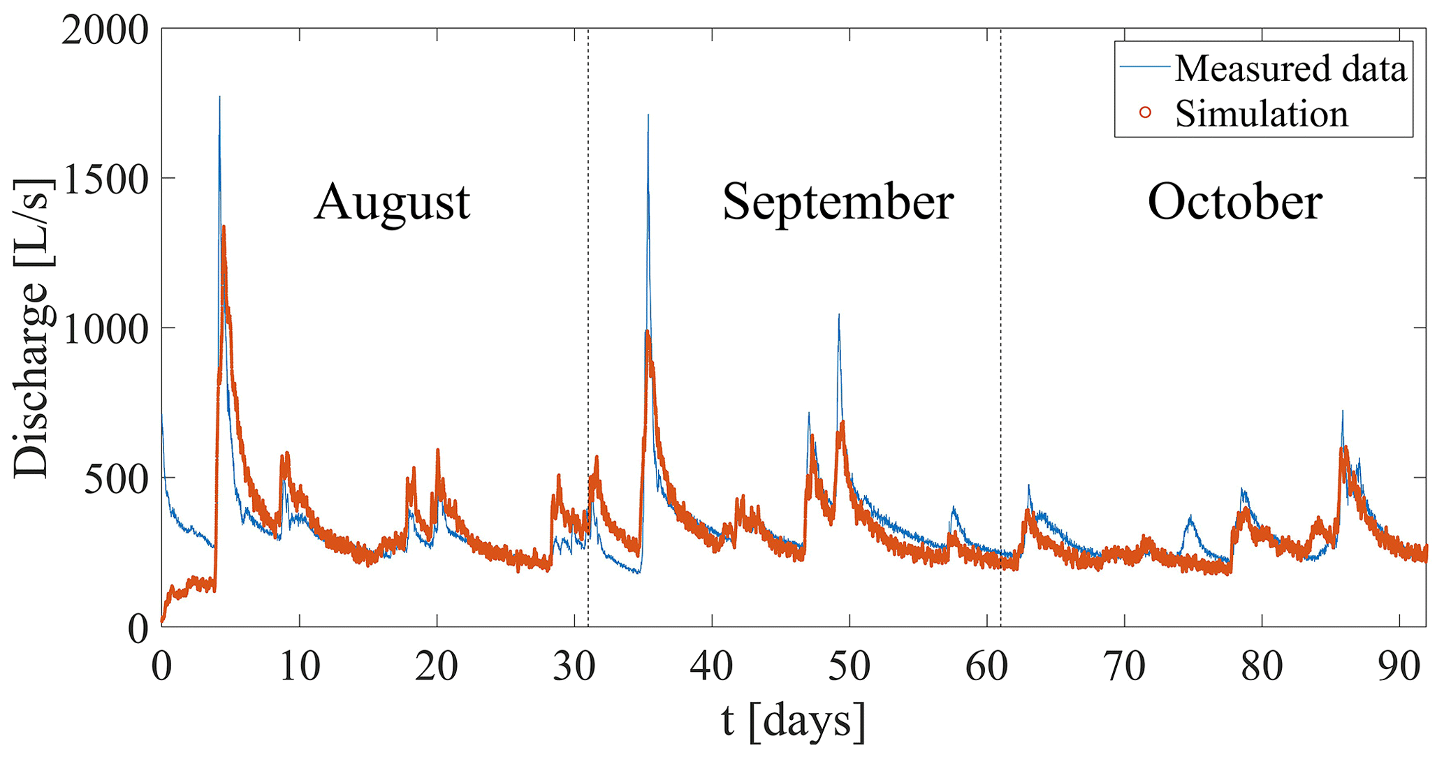
Figure 6 Measured and simulated spring discharge for the 2016 dataset (NSE = 0.5; BE = 0.98).

The differences between the fast- and slow-flow components, as illustrated by the respective optimized CTRW parameters, elucidate the contribution of each flow component to the volumetric discharge. The fast-flow velocity parameter ($v_{\mathit{\psi }}^{\mathrm{f}}$ = 360 m h⁻¹) is much larger than the slow-flow velocity parameter ($v_{\mathit{\psi }}^{\mathrm{s}}$ = 18 m h⁻¹), showing how incoming rain can rapidly flow to the spring outlet (when traveling through the large conduits). The slow diffusive flow, however, has a much longer travel time than the fast flow. Another clear difference between the two components, which is evident from the optimized values, is the degree of anomalous transport. The fast-flow β (1.7) and τ₂ (10⁶) parameters lead to a more symmetrical contribution to the resulting discharge around the peak following the recharge event, compared with the slow-flow parameters (β = 1.2, τ₂ = 10⁸), which create a long tail after the discharge peak. The slow flow is also much more dispersive ($D_{\mathit{\psi }}^{\mathrm{s}}$ = 3.6 × 10⁸ m² h⁻¹) compared with the fast flow ($D_{\mathit{\psi }}^{\mathrm{f}}$ = 36 m² h⁻¹), which contributes further to the long discharge tails. The optimized parameters show a strong prominence of the slow flow over the fast flow: 95 % of newly introduced particles are introduced as slow particles (SF_r), with a 0.01 % likelihood at each iteration of a slow particle transiting to a fast regime (SF_l). The optimized tortuosity factor of 1.6 found for the Disnergschroef system is somewhat higher than that found in some cases (∼ 1.2–1.4, e.g., Jouves et al., 2017; Collon et al., 2017), although well within the range (1.1–3.9) reported for karst systems (e.g., Assari and Mohammadi, 2017). The higher value can be attributed to the morphology of the specific system as well as to the fact that, while tortuosity is often calculated at the cave branch scale (e.g., Jouves et al., 2017; Collon et al., 2017), the CTRW-PT model uses a catchment-scale tortuosity factor. The variability in the tortuosity in different karst morphologies should, therefore, be recognized when considering different modeling scenarios.

The fit obtained for the 2016 dataset modeling is satisfactory considering the inherent uncertainty associated with the input data. The three weather stations used to measure the precipitation are not located inside the catchment area, and different precipitation data were measured at each station, which can be seen by examining the cross-correlation coefficients between the 2016 discharge and rainfall data: 0.20, 0.22, and 0.15 for Koerbersee, Formarinalpe, and Sonntag/Stein stations, respectively (Fig. 2a). While an average of the three stations provides an acceptable estimate of the recharge over the given time period, the variability in local rain events is overlooked, which may be common in the high mountainous topography.

The same set of CTRW parameters optimized for the 2016 data – without further adjustment – was employed to interpret the 2017 and 2018 datasets (Fig. 7). Both datasets show that the simulated discharge after rainfall events predicts the onset, length, and volume of the measured discharge. This is especially true for the many discharge peaks exhibited by the 2018 data.

Figure 7 Measured and simulated spring discharge for the (a) 2017 (NSE = 0.33; BE = 0.98) and (b) 2018 (NSE = 0.63; BE = 0.96) datasets. Note that the vertical scales in Figs. 6 and 7 have been adjusted due to the large differences in maximum discharge among the 3 years.

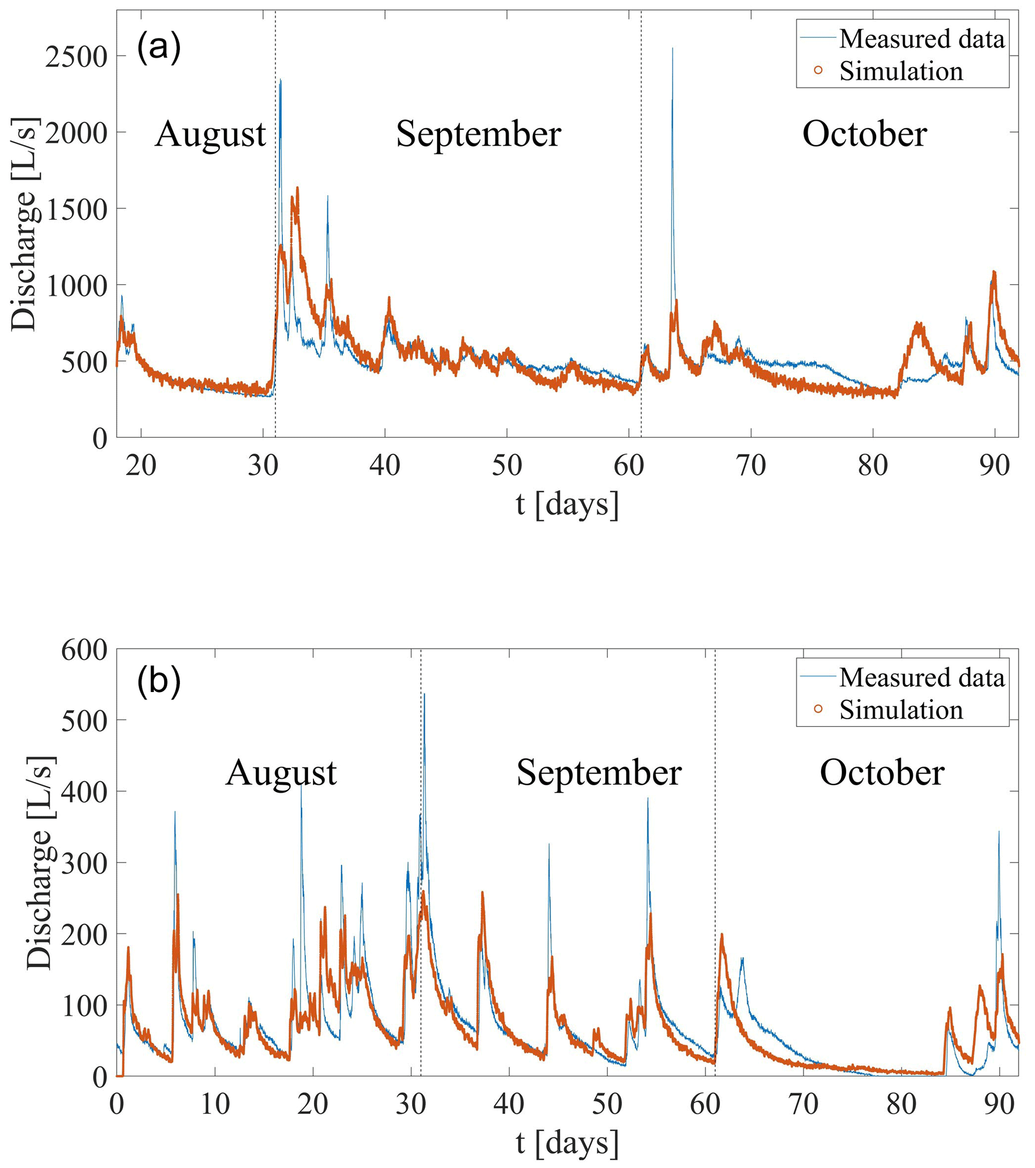
The recharge capacity parameter (applied to calculate the recharge function from the measured rainwater; see Eq. 11) was calculated as 0.43 and 0.45 for the 2016 and 2017 datasets, respectively. These values suggest that ∼ 40 % of the incoming rainfall reaches the outlet spring, with the remaining water reaching deeper parts of the aquifer that are less mobile. The drier 2018 dataset, however, displayed a much lower value of 0.19. The variability in the recharge capacity parameter during different time periods, as a function of the rainfall pattern and amount, highlights the importance of this parameter to the correct prediction of the system discharge response to rainfall.

4.2 Prominence of the slow-flow component in the Disnergschroef system

The prominence of the slow component in this karst system is evident from both the high SF_r and low SF_l. The consistency of this finding, across the three datasets (Figs. 6 and 7), agrees with the analysis of the recharge–discharge relationship by Frank et al. (2021). The aforementioned authors observed that, while the flow from epikarst to conduit and matrix is highly variable and rainfall-dependent, the matrix-to-conduit flow remains relatively constant up to a threshold. The coupling of the two flow processes produces a distinctive discharge pattern characterized by a sharp, rapid peak after a rainfall event, followed by a long tail during recession and a return to baseflow. The current analysis is similar and further emphasizes that the volumetric contribution of the slow flow is substantial, particularly influencing the extended tails. In contrast, the fast flow plays a more straightforward role, contributing predominantly to discharge peaks by quickly expelling introduced rainwater from the system.

Given the importance of karst systems for human consumption, monitoring and prediction of system discharge is especially important during high- and low-flow scenarios. These extreme events can have consequences on water quality, including overconsumption during dry periods and increases in turbidity and bacterial activity under high-flow conditions (Pronk et al., 2006). The frequency of both dry periods and heavy-rainfall events has been shown to rise due to climate change (Stoll et al., 2011), and this may well increase in the near future. In this context, the high peaks and long tails associated with these flow conditions have proven to be the most difficult to correctly predict, across different karst modeling approaches (Jeannin et al., 2021). Here, the results of the CTRW modeling exhibit the long tails associated with low water flow. The 2018 dataset, in particular, which represents a dry summer compared with the other two datasets, exemplifies the robustness of the model with respect to predicting low-flow conditions.

4.3 The contribution of the slow- and fast-flow components to simulated discharge

The results for all three datasets do not show agreement between the maximum simulated and observed discharge values that are found immediately after high-recharge events. The fast response of discharge to the incoming rain in karst systems after high-recharge events has been described in previous studies as a piston effect (Aquilina et al., 2006; Hartmann et al., 2014). Incoming rain creates a rise in discharge before the rainwater reaches the outlet, as the increase in hydraulic head pushes out water that was retained in the system before the rain. This effect was shown specifically in the Disnergschroef system by Frank et el. (2021), who measured a 2.5 h difference between the first response of spring discharge to a rainfall event and the arrival of the rainwater to the outlet. Here, the model does not explicitly take this effect into account, which creates the negative bias in modeling the high peaks. While outside the scope of this study, this feature might be addressed in the future by (1) adding a third flow component or (2) further refining the CTRW parameters of the particles present in the system prior to the rainfall event to represent the increase in flow velocity.

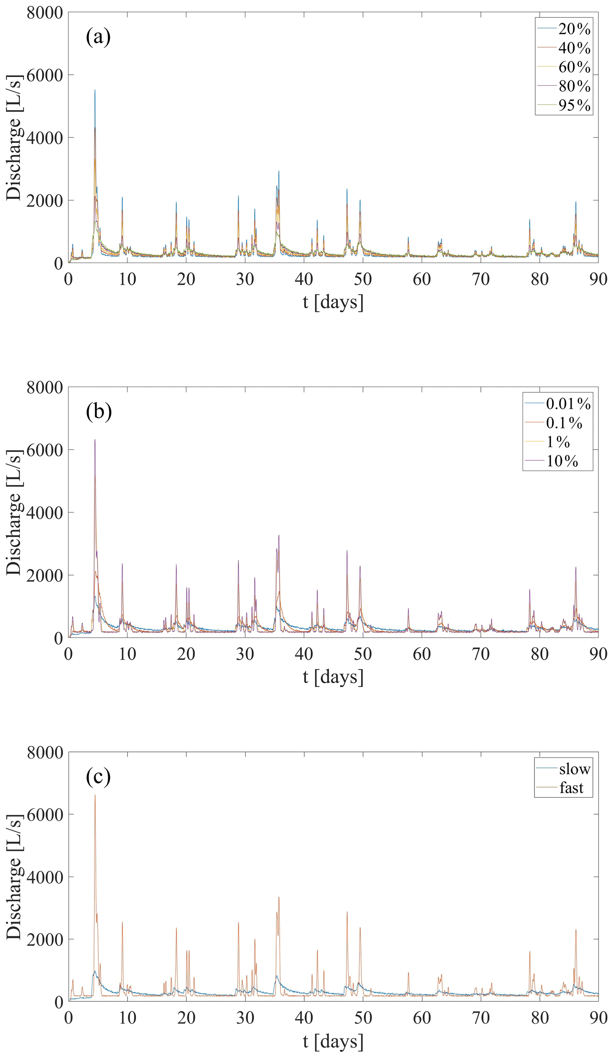
Figure 8 Simulation sensitivity to slow and fast particle contributions, based on the 2016 rainfall data. Simulations that compare (a) different SF_r values, (b) different SF_l values, and (c) only fast/slow particles demonstrate the importance of slow flow with respect to the observed long tails in the discharge data.

To further examine the effect of both the slow- and fast-flow components on the simulated discharge, simulations that examine the SF_l and SF_r parameters across a wider range were conducted (Fig. 8). Simulations that contained only fast or slow particles (Fig. 8a) clearly show that fast-flow discharge responds very quickly to rainfall and produces no observable tails. In contrast, slow flow produces very long tails. It is noteworthy that the first response of the slow flow is similar to the fast flow, as particles that are introduced to the system close to the outlet have a very short length to travel to reach the outlet. Mixing of both flow regimes, either by directly splitting the particles between the two regimes as they are introduced (Fig. 8b) or by changing the transition likelihood (Fig. 8c), produces an intermediate response: as more of the flow is slow, longer tails are found but peaks are smaller. Thus, SF_l and SF_r are important parameters, as they allow for the application of the CTRW-PT model to different karst systems. The Disnergschroef system, presented here as a case study, is characterized by a thick vadose zone and negligible surface runoff. Different karst systems are likely to show different SF_l and SF_r parameters.

5 Conclusions

An analogy between partially saturated water flow in karst aquifers and anomalous chemical transport is established, allowing for the adaptation of the CTRW-PT model to water flow in general as well as for karst discharge response to rainfall specifically. The model was calibrated on one summer season of measurements of spring outlet discharge response to incoming rain; it was then used to predict the long tails observed in discharge measurements following rainfall events in two subsequent summer seasons.

The investigation of the Disnergschroef karst system has shown that slow diffusive flow is a predominant contributor to the volumetric discharge response to recharge events, in comparison to fast conduit flow. This finding highlights the nuanced interplay between fast- and slow-flow components in karst systems as well as how they both evolve over time and as a function of the recharge intensity.

The theoretical and practical advancements presented here offer a potentially robust tool to further assess long-tailed rainfall–discharge responses in karst systems and other complex, catchment-scale systems. The specific application of the CTRW-PT model to the Disnergschroef system has shown that it is particularly advantageous with respect to predicting the long tails observed in discharge data, compared with other modeling approaches.