Power law between the apparent drainage density and the pruning area

Self-similar structures of river networks have been quantified as having diverse scaling laws. Among these, we investigated a power function relationship between the apparent drainage density ρ_a and the pruning area A_p, with an exponent η. We analytically derived the relationship between η and other known scaling exponents of fractal river networks. The analysis of 14 real river networks covering a diverse range of climate conditions and free-flow connectivity levels supports our derivation. We further linked η with non-integer fractal dimensions found for river networks. Synthesis of our findings through the lens of fractal dimensions provides an insight that the exponent η has fundamental roots in the fractal dimension of the whole river network organization.

1 Introduction

Since first being proposed by Horton (1945), the drainage density ρ has long been recognized as an important metric to describe the geomorphological and hydrological characteristics of a catchment. This is defined as $\mathit{\rho }=L_{\mathrm{T}}/A_{\mathrm{T}}$, where A_T is the total catchment area, and so ρ is a function of the total channel length L_T in a catchment. Alternatively, ρ is a function of the channel-forming area A_o (also called the source area or the critical contributing area) (Band, 1986; Montgomery and Dietrich, 1988; Tarboton et al., 1988), which is directly related to L_T. The spatial variation of ρ among catchments is associated with their climates (Melton, 1957; Madduma Bandara, 1974; Wang and Wu, 2013), which can be represented by measures such as the precipitation effectiveness (PE) index (Thornthwaite, 1931). Also, over time, A_o and, thus, ρ of a given catchment dynamically vary. A_o is reduced as the catchment becomes wetter, with water accumulating more readily in the soils of low-gradient areas and saturated areas expanding accordingly. This mechanism leads to the enlargement of the stream network (greater L_T). Conversely, when the catchment gets drier, A_o increases, which in turn results in the contraction of the stream network (Godsey and Kirchner, 2014; Hooshyar et al., 2015; Durighetto et al., 2020). Therefore, L_T and ρ are inversely related to A_o (Tarboton et al., 1991).

On another note, the “rate” at which L_T (and, thus, ρ) varies with A_o is likely to be determined by the shape of landscape or a given topography. The close relationship between the main channel length L and the drainage area A is well known as a power function with a positive exponent h (Hack, 1957); i.e.,

$$\begin{array}{}\text{(1)}& L\propto A^h,\end{array}$$

which provides a clue about the relationship between L_T and A_o. However, these differ in two senses: (1) L_T is the total length counting all tributaries, while L is the length of the main channel only, and (2) L is the length within the area A, while L_T is the length of channels excluded from A_o. L_T is reduced as A_o increases, while L grows with A (Eq. 1).

The usage of digital elevation models (DEMs) in the river network analysis introduced a constant called the pruning area A_p. In extracting a stream network from a DEM, cells of the upslope area A less than A_p are considered to be hillslopes and are excluded from the network. For the ideal delineation of a river network, A_p is expected to be A_o. However, A_p is an arbitrary value and differs from A_o by definition. If A_p=0, every DEM cell is considered to be a channel, while A_p can be as large as A_T for a completely dry landscape. As A_p increases, fewer channels are extracted, resulting in a smaller “apparent” drainage density ρ_a. We distinguish ρ_a from the real drainage density ρ, accommodating the difference between A_p and A_o. It was found that ρ_a decreases as A_p grows, following a power function (Moglen et al., 1998); i.e.,

$$\begin{array}{}\text{(2)}& {\mathit{\rho }}_{\mathrm{a}}\propto A_{\mathrm{p}}^{-\mathit{\eta }},\end{array}$$

where the scaling exponent η>0. While Eq. (2) should be distinguished from the relationship between ρ and A_o, it reflects the topographic characteristic, which is likely to be similar to the relationship between ρ and A_o.

The background described above naturally leads us to the basic question about the physical origin of the power law seen in Eq. (2) and its scaling exponent η. L_T has been expressed as a power function of the discharge at the catchment outlet Q (Godsey and Kirchner, 2014; Hooshyar et al., 2015; Jensen et al., 2017); i.e., L_T∝Q^β. Prancevic and Kirchner (2019) derived the exponent β as the combination of η and two other scaling exponents found in topographic attributes; i.e., $\mathit{\beta }=\mathit{\eta }/(\mathit{\theta }+\mathit{\gamma }+\mathrm{1})$, where θ is the power-law exponent relating local channel slope to drainage area (called the concavity) (Montgomery and Foufoula-Georgiou, 1993; McNamara et al., 2006), and γ is the exponent of a hypothetical power function between A and valley transmissivity T (the product of a subsurface cross-sectional area and conductivity, which in turn is expressed in units of cubic length per time) (Prancevic and Kirchner, 2019). Adopting this, we can reason that $\mathit{\eta }=\mathit{\beta }(\mathit{\theta }+\mathit{\gamma }+\mathrm{1})$. However, Prancevic and Kirchner (2019) acknowledged that the above expression of β is yet to be generalized across a range of sizes and landscapes. Equation (2) and the exponent η are awaiting deeper investigations.

Moglen et al. (1998) attempted direct DEM analyses to investigate the ρ_a–A_p relationships in real river networks. However, A_o and A_p were not distinguished, and little discussion about η was given. Furthermore, the topographic data they adopted were limited, and a greater-resolution DEM for catchments of known A_o and/or blue-line data are needed to properly approach the given subject with terrain analyses. It is worth realizing that the power-law relationship of Eq. (2) implies fractal network formation. A river network is fractal, and many regular power laws have been reported as being characteristic signatures of a naturally evolved river network (Dodds and Rothman, 2000). As the power-law relationship between ρ_a and A_p can also serve as a signature reflecting the self-similarity, it is plausible to make a claim regarding the linkage between the ρ_a–A_p relationship and other power laws known in natural river networks.

The exponent η brings further interesting questions. In Eq. (2), η=0.5 is anticipated to satisfy dimensional consistency (Tarboton et al., 1991). However, the rough analysis of Moglen et al. (1998) raises doubts as to whether η estimated from any real catchment meets this consistency. This issue is analogous to the question about the exponent h in Eq. (1), which should also be 0.5 to keep consistency in terms of dimension (Hjelmfelt, 1988). In fact, h values reported for natural rivers are mostly greater than 0.5, i.e., between 0.5 and 0.7 (Hack, 1957; Gray, 1961; Robert and Roy, 1990; Crave and Davy, 1997). This has brought about the introduction of the fractal dimension (Mandelbrot, 1977), whose values for river networks range between 1 and 2 (e.g., Feder, 1988) (further detailed explanations are provided in Sect. 4). Similarly, we can claim that the dimensional inconsistency in Eq. (2), if any, can be resolved by incorporating the fractal dimension. It is also an open question as to what controls η. While the relationship between ρ_a and A_p reflects the topography, if η is a fixed constant of 0.5 then, despite dimensional consistency, this implies a limited role of topographic variations in η. If η is variable, the underpinning mechanism that changes the local catchment topography and, thus, η is to be explored. In particular, we are curious about the roles of human intervention and ecosystem evolution in conjunction with climate forcing in the relationship between ρ_a and A_p. To understand this, we desire to investigate a range of catchments under different developmental stages and climate conditions.

Here, we aimed to corroborate the aforementioned claims and hypotheses about the ρ_a–A_p relationship and its exponent η. To this end, in Sect. 2, we review the known scaling relationships in a river network. Then, we present an analytical derivation of Eq. (2) and demonstrate how this is related to other power laws known for a river network. To support our argument, many real catchments under the wide range of climatic conditions and free-flow connectivity levels were analyzed with terrain analysis methods in a thorough manner using high-resolution DEMs and trustworthy blue-line data. These are described in Sect. 3. With these results, we explore the physical meanings embedded in the power-law relationship between ρ_a and A_p with the notion of a fractal dimension in Sect. 4. A summary and conclusions are given in Sect. 5.

2 Cross-relationships among scaling laws

2.1 Review of the scaling laws of a river network

The river network has been perceived to be an archetypal fractal network in nature (Mandelbrot, 1977; Rodríguez-Iturbe and Rinaldo, 2001), exhibiting scale-invariant organization. Systematic measures for characterizing structural hierarchy help to manifest the self-similarity. The Horton–Strahler ordering scheme (Horton, 1945; Strahler, 1957) has been popularly employed to investigate the structural characteristics of river networks. In this framework, the number, the mean length, and the mean drainage area of ω-order streams in a catchment – stated as N_ω, ${\stackrel{\mathrm{‾}}{L}}_{\mathit{\omega }}$, and ${\stackrel{\mathrm{‾}}{A}}_{\mathit{\omega }}$, respectively – are defined for an order ω ranging from 1 to Ω, where Ω is the highest order in the network. There is only one Ω-order stream in a river network (i.e., N_Ω=1). Then, the total channel length L_T used for the definition of the drainage density ρ is given as

$$\begin{array}{}\text{(3)}& L_{\mathrm{T}}=\sum _{\mathit{\omega }=\mathrm{1}}^{\mathrm{\Omega }}{N}_{\mathit{\omega }}{\stackrel{\mathrm{‾}}{L}}_{\mathit{\omega }}.\end{array}$$

Following its definition, the length of any lower-order stream is excluded in ${\stackrel{\mathrm{‾}}{L}}_{\mathit{\omega }}$. Therefore, ${\stackrel{\mathrm{‾}}{L}}_{\mathrm{\Omega }}$ is neither the upslope length L of a main channel nor L_T. In contrast, ${\stackrel{\mathrm{‾}}{A}}_{\mathit{\omega }}$ includes the drainage area of all upstream branches (of ω−1 and lower orders); e.g., ${\stackrel{\mathrm{‾}}{A}}_{\mathrm{\Omega }}$ is identical to A_T. To resolve the discrepant definitions of ${\stackrel{\mathrm{‾}}{L}}_{\mathit{\omega }}$ and ${\stackrel{\mathrm{‾}}{A}}_{\mathit{\omega }}$, the cumulative mean length Γ_ω was proposed to match the definition of area (Broscoe, 1959) as

$$\begin{array}{}\text{(4)}& {\mathrm{\Gamma }}_{\mathit{\omega }}=\sum _{k=\mathrm{1}}^{\mathit{\omega }}{\stackrel{\mathrm{‾}}{L}}_k,\end{array}$$

which is an order-discretized approximation of L. Alternatively, to match the definition of length, the eigenarea, also called the interbasin area (Strahler, 1964) or the contiguous area (Marani et al., 1991), was proposed as the area draining directly into the ω-order stream (Beer and Borgas, 1993). The mean eigenarea ${\stackrel{\mathrm{‾}}{E}}_{\mathit{\omega }}$ of ω-order streams is

$$\begin{array}{}\text{(5)}& {\stackrel{\mathrm{‾}}{E}}_{\mathit{\omega }}={\stackrel{\mathrm{‾}}{A}}_{\mathit{\omega }}-{\stackrel{\mathrm{‾}}{A}}_{\mathit{\omega }-\mathrm{1}}\left(N_{\mathit{\omega }-\mathrm{1}}/N_{\mathit{\omega }}\right).\end{array}$$

The self-similar structure of a river network has been captured through the linear scaling of the above quantities (N_ω, ${\stackrel{\mathrm{‾}}{L}}_{\mathit{\omega }}$ ${\stackrel{\mathrm{‾}}{A}}_{\mathit{\omega }}$, and ${\stackrel{\mathrm{‾}}{E}}_{\mathit{\omega }}$) with ω on a semi-log paper (Horton, 1945; Schumm, 1956; Yang and Paik, 2017):

$$\begin{array}{}\text{(6)}& \begin{array}{rl}{N}_{\mathit{\omega }}=& R_{\mathrm{B}}^{\mathrm{\Omega }-\mathit{\omega }},{\stackrel{\mathrm{‾}}{L}}_{\mathit{\omega }}={\stackrel{\mathrm{‾}}{L}}_{\mathrm{\Omega }}{R}_{\mathrm{L}}^{\mathit{\omega }-\mathrm{\Omega }},{\stackrel{\mathrm{‾}}{A}}_{\mathit{\omega }}={\stackrel{\mathrm{‾}}{A}}_{\mathrm{\Omega }}{R}_{\mathrm{A}}^{\mathit{\omega }-\mathrm{\Omega }},\\ & \mathrm{and}{\stackrel{\mathrm{‾}}{E}}_{\mathit{\omega }}={\stackrel{\mathrm{‾}}{E}}_{\mathrm{\Omega }}{R}_{\mathrm{E}}^{\mathit{\omega }-\mathrm{\Omega }},\end{array}\end{array}$$

where R_B, R_L, R_A, and R_E are the bifurcation, the length, the area, and the eigenarea ratios, respectively. These dimensionless ratios are often called the Horton ratios as a group. They are related to each other (Morisawa, 1962; Rosso, 1984; Tarboton et al., 1990; Yang and Paik, 2017) and typically show the ranges $\mathrm{3}<R_{\mathrm{B}}<\mathrm{5}$, $\mathrm{1.5}<R_{\mathrm{L}}\approx R_{\mathrm{E}}<\mathrm{3}$, $\mathrm{3}<R_{\mathrm{A}}<\mathrm{6}$ (Smart, 1972), and R_E≈R_L (Yang and Paik, 2017).

In addition to Eq. (6), power function relationships between geomorphologic variates have also been found and have served as evidence of the scale-invariant river network structures. Hack's law (Eq. 1) is a classical principle in this regard. Another interesting power-law relationship lies in the exceedance probability distributions of upstream areas. Using a theoretical aggregation model, Takayasu et al. (1988) showed that the exceedance probability distribution of injected mass in a tree network always follows a power law. In fact, their model is equivalent to the random-walk model of Scheidegger (1967), devised to mimic a river network (Takayasu and Nishikawa, 1986). Replacing the mass (flow) in the aforementioned study with the drainage area (which is rational if rainfall is spatially uniform) leads to the power-law exceedance probability distribution of drainage area. From all DEM cells composing a catchment, one can calculate the probability distribution of the upslope area A of a cell, i.e., P(A), which is minimal for A=A_T (as only one cell at the outlet meets this case). It is found that the probability for a randomly designated point having A exceeding a reference value δ ($\mathrm{0}\le \mathit{\delta }\le A_{\mathrm{T}}$) decreases with δ (Rodríguez-Iturbe et al., 1992a), following a power law as follows:

$$\begin{array}{}\text{(7)}& P(A\ge \mathit{\delta })\propto {\mathit{\delta }}^{-\mathit{\epsilon }},\end{array}$$

where the exponent ε is reported as being between 0.40 and 0.46 for most river networks (Rodríguez-Iturbe et al., 1992a; Crave and Davy, 1997). The two power laws, in Eqs. (1) and (7), are related with $h+\mathit{\epsilon }=\mathrm{1}$ (Maritan et al., 1996), which suggests a trade-off between the two exponents by balancing each other with their respective ranges to form the catchment boundary within a confined space.

The two classes of scaling relationships reviewed above, i.e., Horton's laws (Eq. 6) and power-law relationships, are linked as shown by La Barbera and Roth (1994); i.e.,

$$\begin{array}{}\text{(8)}& \mathit{\epsilon }=\mathrm{1}-h={\displaystyle \frac{\ln \left(R_{\mathrm{B}}/R_{\mathrm{L}}\right)}{\ln R_{\mathrm{A}}}}.\end{array}$$

Two other expressions, comparable to Eq. (8), appear in the literature; de Vries et al. (1994) derived $\mathit{\epsilon }=\mathrm{1}-\ln R_{\mathrm{L}}/\ln R_{\mathrm{B}}$, which is a special case of Eq. (8) where R_B=R_A. Empirical studies support that R_B is indeed close to R_A (Smart, 1972). For a “topological” Hortonian tree where no constraint on stream length in a finite area is given, Veitzer et al. (2003) and Paik and Kumar (2007) showed that $\mathit{\epsilon }=\ln R_{\mathrm{B}}/\ln R_{\mathrm{A}}-\mathrm{1}$. This is another special case of Eq. (8) where R_L=R_A, the assumption used in the analysis of topological self-similar trees where only connections among nodes matter with no spatial constraint (Paik and Kumar, 2007).

2.2 Linkage to ρ_a–A_p relationship

The inverse relationship between the pruning area A_p and the resulting apparent drainage density ρ_a can be found in the DEM analysis (Fig. 1). Below, we analytically derived their plausible relationship (Eq. 2) using the scaling relationships reviewed above. Through this investigation, we importantly revealed that η=ε; i.e., the scaling exponents in Eqs. (2) and (7) are identical. We arrived at the same conclusion using two different approaches, as described below.

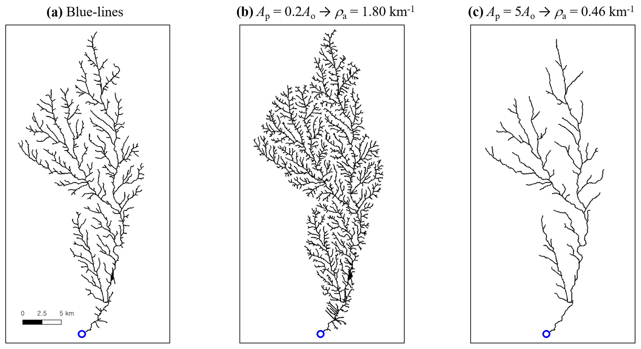
Figure 1 Stream network (black line) of the Brushy catchment, USA, extracted with varying pruning area. A blue circle indicates the outlet. For this catchment, the channel-forming area A_o and the corresponding drainage density ρ are available from the National Hydrography Dataset Plus Version 2 (NHDPlusV2) (McKay et al., 2012) (see Sect. 3 for details). (a) Blue lines of the Brushy River network as given in the NHDPlusV2, with A_o=0.14 km² and ρ_a=0.97 km⁻¹. (b, c) Extension and contraction of the river network with a pruning area A_p that is 5 times smaller and greater than A_o, respectively. The apparent drainage density ρ_a accordingly varies.

2.2.1 Derivation 1

For the Hortonian tree, A_p can vary in a discrete manner (order by order) as we set $A_{\mathrm{p}}={\stackrel{\mathrm{‾}}{A}}_{\mathit{\omega }}$. Given that up to ω-order streams are pruned in a river network, the total length after pruning is $\sum _{k=\mathit{\omega }+\mathrm{1}}^{\mathrm{\Omega }}{N}_k{\stackrel{\mathrm{‾}}{L}}_k$, revising Eq. (3). Replacing N_k and ${\stackrel{\mathrm{‾}}{L}}_k$ in this equation with the elements in Eq. (6) leads to the expression of ρ_a as

$$\begin{array}{}\text{(9)}& {\mathit{\rho }}_{\mathrm{a}}={\displaystyle \frac{{\stackrel{\mathrm{‾}}{L}}_{\mathrm{\Omega }}}{{\stackrel{\mathrm{‾}}{A}}_{\mathrm{\Omega }}}}\sum _{k=\mathit{\omega }+\mathrm{1}}^{\mathrm{\Omega }}{R}_{\mathrm{B}}^{\mathrm{\Omega }-k}{R}_{\mathrm{L}}^{k-\mathrm{\Omega }}.\end{array}$$

The sum of the above geometric series is

$$\begin{array}{}\text{(10)}& {\mathit{\rho }}_{\mathrm{a}}={\displaystyle \frac{{\stackrel{\mathrm{‾}}{L}}_{\mathrm{\Omega }}}{{\stackrel{\mathrm{‾}}{A}}_{\mathrm{\Omega }}\left(R_{\mathrm{B}}/R_{\mathrm{L}}-\mathrm{1}\right)}}\left[{\left({\displaystyle \frac{R_{\mathrm{B}}}{R_{\mathrm{L}}}}\right)}^{\mathrm{\Omega }-\mathit{\omega }}-\mathrm{1}\right].\end{array}$$

The logarithm of the term $(R_{\mathrm{B}}/R_{\mathrm{L}}{)}^{\mathrm{\Omega }-\mathit{\omega }}$ in Eq. (10) can be written, using Eq. (6), as

$$\begin{array}{}\text{(11)}& \begin{array}{rl}\ln {\left({\displaystyle \frac{R_{\mathrm{B}}}{R_{\mathrm{L}}}}\right)}^{\mathrm{\Omega }-\mathit{\omega }}& =(\mathrm{\Omega }-\mathit{\omega })\ln {\displaystyle \frac{R_{\mathrm{B}}}{R_{\mathrm{L}}}}={\displaystyle \frac{\ln \left({\stackrel{\mathrm{‾}}{A}}_{\mathrm{\Omega }}/{\stackrel{\mathrm{‾}}{A}}_{\mathit{\omega }}\right)}{\ln R_{\mathrm{A}}}}\ln {\displaystyle \frac{R_{\mathrm{B}}}{R_{\mathrm{L}}}}\\ & ={\displaystyle \frac{\ln \left(R_{\mathrm{B}}/R_{\mathrm{L}}\right)}{\ln R_{\mathrm{A}}}}\ln {\displaystyle \frac{{\stackrel{\mathrm{‾}}{A}}_{\mathrm{\Omega }}}{{\stackrel{\mathrm{‾}}{A}}_{\mathit{\omega }}}}.\end{array}\end{array}$$

Given that ${\stackrel{\mathrm{‾}}{A}}_{\mathit{\omega }}=A_{\mathrm{p}}$ from Eq. (11), we can state

$$\begin{array}{}\text{(12)}& {\left(R_{\mathrm{B}}/R_{\mathrm{L}}\right)}^{\mathrm{\Omega }-\mathit{\omega }}={\left({\stackrel{\mathrm{‾}}{A}}_{\mathrm{\Omega }}/A_{\mathrm{p}}\right)}^{\frac{\ln \left(R_{\mathrm{B}}/R_{\mathrm{L}}\right)}{\ln R_{\mathrm{A}}}}.\end{array}$$

Substituting this into Eq. (10) yields an approximate power law; i.e.,

$$\begin{array}{}\text{(13)}& \begin{array}{rl}{\mathit{\rho }}_{\mathrm{a}}& ={\displaystyle \frac{{\stackrel{\mathrm{‾}}{L}}_{\mathrm{\Omega }}}{{\stackrel{\mathrm{‾}}{A}}_{\mathrm{\Omega }}\left(R_{\mathrm{B}}/R_{\mathrm{L}}-\mathrm{1}\right)}}\left[{\left({\displaystyle \frac{A_{\mathrm{p}}}{{\stackrel{\mathrm{‾}}{A}}_{\mathrm{\Omega }}}}\right)}^{-\frac{\ln \left(R_{\mathrm{B}}/R_{\mathrm{L}}\right)}{\ln R_{\mathrm{A}}}}-\mathrm{1}\right]\\ & \propto A_{\mathrm{p}}^{-\frac{\ln \left(R_{\mathrm{B}}/R_{\mathrm{L}}\right)}{\ln R_{\mathrm{A}}}}.\end{array}\end{array}$$

Given that $R_{\mathrm{B}}\approx R_{\mathrm{A}}>R_{\mathrm{L}}$ (Smart, 1972) for a typical river network, $-\mathrm{1}<-\ln (R_{\mathrm{B}}/R_{\mathrm{L}})/\ln R_{\mathrm{A}}<\mathrm{0}$. With this range and for $A_{\mathrm{p}}\ll {\stackrel{\mathrm{‾}}{A}}_{\mathrm{\Omega }}$, $(A_{\mathrm{p}}/{\stackrel{\mathrm{‾}}{A}}_{\mathrm{\Omega }}{)}^{-\ln (R_{\mathrm{B}}/R_{\mathrm{L}})/\ln R_{\mathrm{A}}}=({\stackrel{\mathrm{‾}}{A}}_{\mathrm{\Omega }}/A_{\mathrm{p}}{)}^{\ln (R_{\mathrm{B}}/R_{\mathrm{L}})/\ln R_{\mathrm{A}}}\gg \mathrm{1}$. This allows the approximation $\left[\right({\stackrel{\mathrm{‾}}{A}}_{\mathrm{\Omega }}/A_{\mathrm{p}}{)}^{\ln (R_{\mathrm{B}}/R_{\mathrm{L}})/\ln R_{\mathrm{A}}}-\mathrm{1}]\approx ({\stackrel{\mathrm{‾}}{A}}_{\mathrm{\Omega }}/A_{\mathrm{p}}{)}^{\ln (R_{\mathrm{B}}/R_{\mathrm{L}})}/\ln R_{\mathrm{A}}$. Empirical studies suggested $A_{\mathrm{o}}<\mathrm{0.1}{\stackrel{\mathrm{‾}}{A}}_{\mathrm{\Omega }}$ to characterize fluvial channel networks (Montgomery and Foufoula-Georgiou, 1993; McNamara et al., 2006), implying the scope of this derivation, i.e., $A_{\mathrm{p}}\ll {\stackrel{\mathrm{‾}}{A}}_{\mathrm{\Omega }}$, to be of a practical range. Comparing Eqs. (2) and (13), we can explicitly express

$$\begin{array}{}\text{(14)}& \mathit{\eta }={\displaystyle \frac{\ln \left(R_{\mathrm{B}}/R_{\mathrm{L}}\right)}{\ln R_{\mathrm{A}}}}.\end{array}$$

This expression is identical to Eq. (8), which implies η=ε.

2.2.2 Derivation 2

The conclusion of η=ε can also be derived by employing the eigenarea (Yang, 2016). Approximating an ω-order sub-catchment as a rectangle, ${\stackrel{\mathrm{‾}}{E}}_{\mathit{\omega }}$ can be rewritten as ${\stackrel{\mathrm{‾}}{E}}_{\mathit{\omega }}=W{\stackrel{\mathrm{‾}}{L}}_{\mathit{\omega }}$, where the mean overland flow length is $W/\mathrm{2}$. As W is regarded to be almost a constant (Hack, 1957; Yang and Paik, 2017), the apparent drainage density for the pruning area $A_{\mathrm{p}}={\stackrel{\mathrm{‾}}{A}}_{\mathit{\omega }}$ becomes

$$\begin{array}{}\text{(15)}& {\mathit{\rho }}_{\mathrm{a}}={\displaystyle \frac{\mathrm{1}}{{\stackrel{\mathrm{‾}}{A}}_{\mathrm{\Omega }}}}\sum _{k=\mathit{\omega }+\mathrm{1}}^{\mathrm{\Omega }}{N}_k{\stackrel{\mathrm{‾}}{L}}_k={\displaystyle \frac{\mathrm{1}}{{\stackrel{\mathrm{‾}}{A}}_{\mathrm{\Omega }}W}}\sum _{k=\mathit{\omega }+\mathrm{1}}^{\mathrm{\Omega }}{N}_k{\stackrel{\mathrm{‾}}{E}}_k.\end{array}$$

On the other hand, P(A≥A_p) is defined from geometry as

$$\begin{array}{}\text{(16)}& P\left(A\ge A_{\mathrm{p}}\right)={\displaystyle \frac{\mathrm{1}}{{\stackrel{\mathrm{‾}}{A}}_{\mathrm{\Omega }}}}\sum _{k=\mathit{\omega }+\mathrm{1}}^{\mathrm{\Omega }}{N}_k{\stackrel{\mathrm{‾}}{E}}_k,\end{array}$$

which is equal to Wρ_a from Eq. (15). As $P(A\ge A_{\mathrm{p}})\propto A_{\mathrm{p}}^{-\mathit{\epsilon }}$ (Eq. 7), we realize that ${\mathit{\rho }}_{\mathrm{a}}\propto A_{\mathrm{p}}^{-\mathit{\epsilon }}$, and, thereby, η=ε. While Eq. (13) was derived for $A_{\mathrm{p}}\ll {\stackrel{\mathrm{‾}}{A}}_{\mathrm{\Omega }}$, this alternative derivation shows the power law regardless of the range in A_p. Earlier, we discussed the reciprocal nature of two relationships, one between L_T and A_o and the other between L and A. Combining the above conclusions of η=ε and $h+\mathit{\epsilon }=\mathrm{1}$, we realize that $\mathit{\eta }=\mathrm{1}-h$, which, indeed, implies the compensating function between them.

3 Analyses of real river networks

3.1 Data and methods

We evaluate the power law shown in Eq. (2) with the derivation of η=ε for real river networks in the contiguous United States. We have chosen 14 study networks (Fig. 2) from the pool investigated in the previous studies of Tarboton et al. (1991), Rodríguez-Iturbe et al. (1992a), Botter et al. (2007), Hosen et al. (2021), and Carraro and Altermatt (2022). These were carefully selected to cover distinct hydro-climatic regions and a range of free-flowing capacities (Table 1). The climate feature is described by the Köppen–Geiger climate classification (Beck et al., 2018). The free-flow characteristic is referred to using an integrated connectivity status index (CSI) created at a global scale by Grill et al. (2019) for the first time. The CSI comprehensively and quantitatively describes the capacity of individual river reaches to freely flow based on the synthesis of observed and modeled datasets. The reported CSI values, ranging from 0 % to 100 %, are the weighted average of five estimated pressure indicators – river fragmentation, flow regulation, sediment trapping, water consumption, and infrastructure development in riparian areas and floodplains – which represent natural and human inferences within longitudinal, lateral, vertical, and temporal dimensions. If a river reach loses connectivity due to any of the aforementioned pressures, its CSI value decreases. We calculated a catchment unit CSI by weighting the length of individual reaches in a given catchment. The CSI of our 14 catchments ranges from 58 % to 100 %, which is irrelevant to the catchment size.

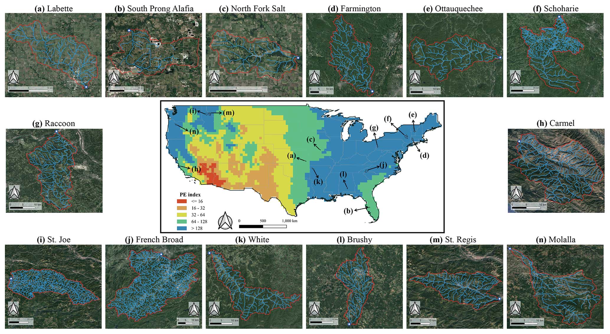
Figure 2 Structure and location of 14 river networks investigated in this study. The central map displays their geographic locations in the contiguous US, overlaid with the spatial PE index distribution. Layouts of individual river networks surround the map, labeled from (a)–(n), corresponding to the order in Table 1. A circular mark in each figure represents the catchment outlet. The river network layouts (light-blue lines) originate from the NHDPlusV2. Satellite images in the background of the study areas were obtained from © Google Earth 2023.

Table 1 Topographic characteristics of the 14 river networks analyzed in this study.

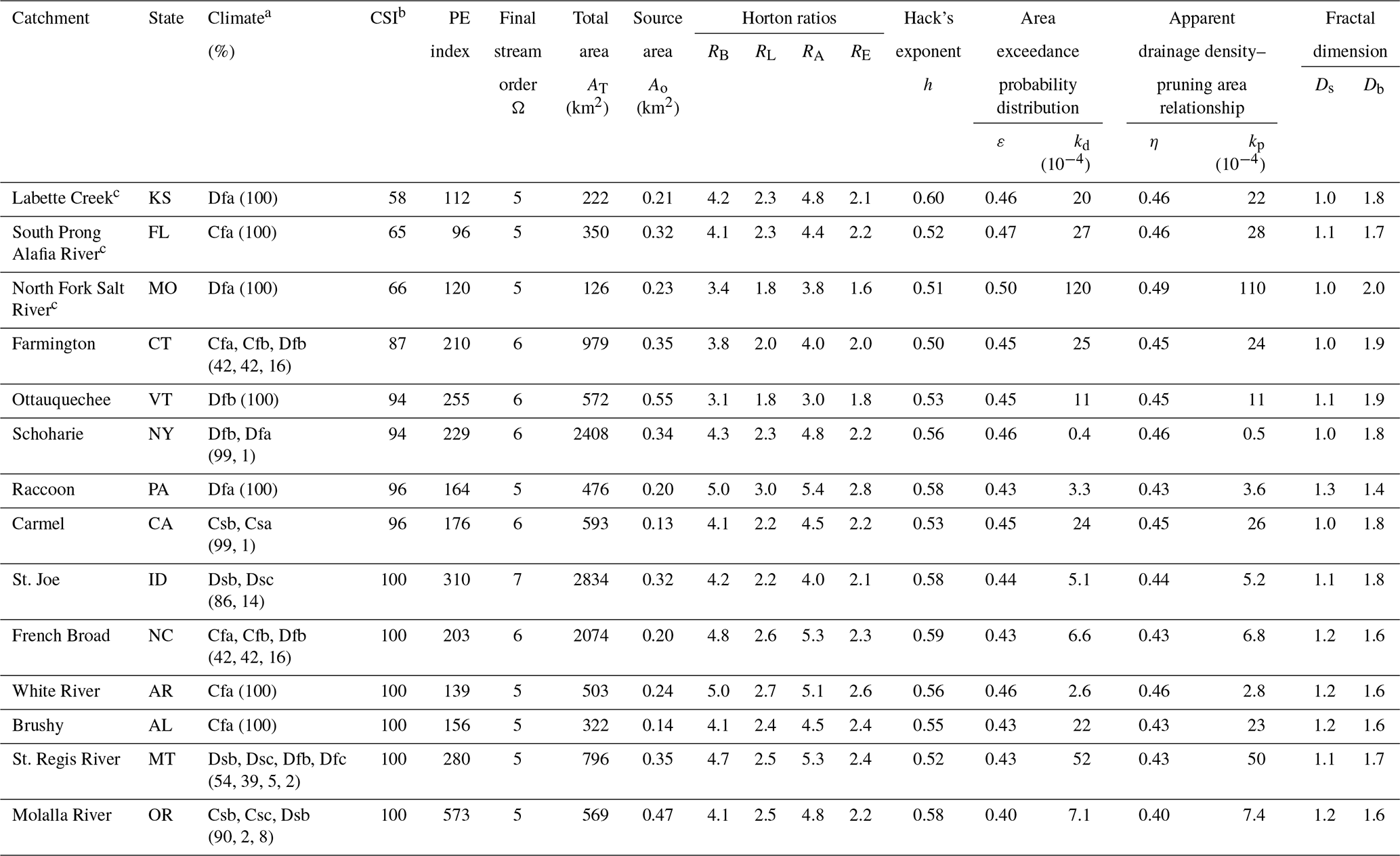
^a Climate zone was based on the Köppen climate classification scheme. ^b The reported connectivity status index (CSI) was weighted by stream length for a given CSI. ^c Catchment name was taken from Open Street Map to be a creek or stream name at the outlet.

To shape the structure of each river network in the grid domain, we used the 1 arcsec raster data of flow direction and upslope area provided in the National Hydrography Dataset Plus Version 2 (NHDPlusV2) (McKay et al., 2012). In the NHDPlusV2, the Deterministic 8 method (O'Callaghan and Mark, 1984) is used for flow direction assignment. The flow direction extraction algorithm is underpinned by the principles of maximizing energy dissipation in surface water flow and minimizing power in groundwater flow (Schiavo et al., 2022). The DEM was processed to discard depression or sink cells. Accordingly, upslope area was calculated for each cell. For detailed calculation steps and processes, readers may refer to the user guide of NHDPlusV2. To extract river networks most resembling individual blue lines, we referred to the source areas recorded in the NHDPlusV2. In the NHDPlusV2, a channel-forming area $A_{\mathrm{o}}^{*}$ is given for stream channels at the most upstream points of individual flow paths in each river network. This is very detailed information, while A_o, as we refer to it, is a single value which represents the entire network. We draw the probability distribution of $A_{\mathrm{o}}^{*}$ for each catchment (Fig. S1 in the Supplement), and A_o was determined as the median (Table 1). The Horton–Strahler ordering was assigned for the pruned river networks.

To investigate any impact of climatic forcing on Eq. (2), we analyzed the PE index (Thornthwaite, 1931), which is defined as the sum of the ratio of mean monthly precipitation to mean monthly potential evaporation (Wang and Wu, 2013). Note that a higher PE index indicates more moisture being available for plant growth. We utilized precipitation and potential evapotranspiration data from the Climatic Research Unit time series (CRU TS) on high-resolution 0.5°-by-0.5° grids at the global scale (CRU TS v. 4.06 in Harris et al., 2022) for the 50-year period from 1970 to 2019. The CRU dataset is compiled from a comprehensive collection of observations made at weather stations.

Drawing the exceedance probability distribution of the upstream area, i.e., P(A≥δ), for a real catchment in log–log scale, three segments are often characterized: curved head, straight trunk, and truncated tail. The power law (Eq. 7) holds for the straight trunk, which indicates channels. The head reflects hillslope (Moglen and Bras, 1995; Maritan et al., 1996). As A approaches A_T, the probability rapidly drops because the size of a network is finite (Rodríguez-Iturbe et al., 1992a; Moglen et al., 1998; Perera and Willgoose, 1998). To combine the channel part and the truncated tail in the distribution function, the exponentially tempered power function was adopted (Aban et al., 2006; Rinaldo et al., 2014):

$$\begin{array}{}\text{(17)}& P(A\ge \mathit{\delta })=c_{\mathrm{d}}{\mathit{\delta }}^{-\mathit{\epsilon }}\exp \left(-k_{\mathrm{d}}\mathit{\delta }\right)\mathrm{for}\mathit{\delta }>A_{\mathrm{o}},\end{array}$$

where c_d is a constant, and k_d is the tempering parameter. As k_d approaches zero, the function represents abrupt truncation. Similarly, we proposed an exponentially truncated power function for ρ_a, using a general form of Eq. (2), as follows:

$$\begin{array}{}\text{(18)}& {\mathit{\rho }}_{\mathrm{a}}=c_{\mathrm{p}}{A}_{\mathrm{p}}^{-\mathit{\eta }}\exp \left(-k_{\mathrm{p}}{A}_{\mathrm{p}}\right)\mathrm{for}{A}_{\mathrm{p}}>A_{\mathrm{o}},\end{array}$$

where c_p is a constant, and k_p is the tempering parameter. To estimate the best-fitting parameters, we employed MATLAB's nlinfit function, which is designed for nonlinear regression for a given dataset. The objective of the function is to minimize the sum of the squares of the residuals for a defined nonlinear model. The estimated range for a parameter was calculated with 95 % confidence intervals.

3.2 Results and discussion

All studied networks follow well Hack's law, shown in Eq. (1) (Fig. S2). The range of the estimated Hack's exponent h is 0.55±0.03 (mean ± standard deviation), with R²>0.95 (Table 1), which is within the typical range shown in earlier studies (Hack, 1957). The laws of stream number, length, drainage area, and eigenarea (Eq. 6) are satisfied for all study networks, with R²>0.85 (Figs. S3 and S4). The resultant Horton ratios show ranges of $R_{\mathrm{B}}=\mathrm{4.2}\pm \mathrm{0.5}$, $R_{\mathrm{L}}=\mathrm{2.3}\pm \mathrm{0.3}$, and $R_{\mathrm{A}}=\mathrm{4.6}\pm \mathrm{0.7}$ (Table 1), which are within typical ranges (Horton, 1945; Schumm, 1956; Smart, 1972). Further, $R_{\mathrm{E}}=\mathrm{2.2}\pm \mathrm{0.3}$, supporting the argument that R_E≈R_L (Yang and Paik, 2017). These imply that our study networks hold statistically robust self-similar features.

In the exceedance probability distributions of upstream area, three segments of curved head, straight trunk, and truncated tail are clearly characterized for all study catchments (Fig. S5). The visual interpretation is well demonstrated by the results of parameters fitted through Eq. (17) (mean-squared error values < $\mathrm{2}\times {\mathrm{10}}^{-\mathrm{8}}$). The tempering parameter k_d values are very small for all river networks, indicating an abrupt truncation in the tail part (Table 1 and Fig. S5b). The power-law exponent ε shows a range of 0.45±0.02 (Table 1), which agrees with the range reported in earlier studies (e.g., Rodríguez-Iturbe et al., 1992a). The ε values estimated in our study networks satisfy the coupled relation with Hack's exponent h, resulting in $\mathit{\epsilon }+h=\mathrm{1.00}\pm \mathrm{0.03}$.

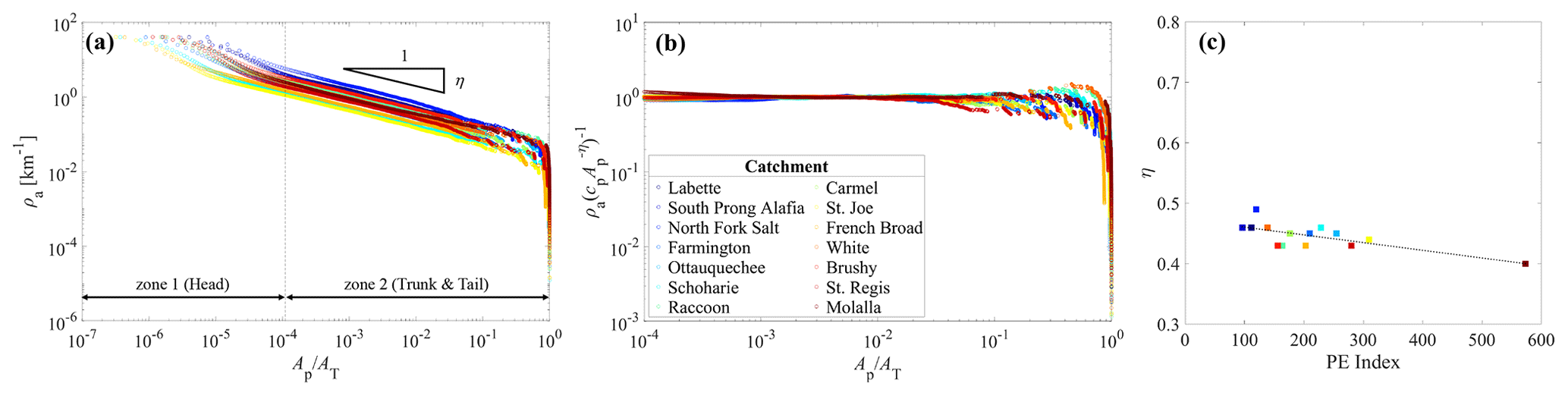
Figure 3 Analyses between the apparent drainage density ρ_a and the pruning area A_p for 14 studied catchments. Color codes for each catchment are maintained consistently across all three panels presented herein. (a) Variation in ρ_a with A_p normalized by A_T in a log–log scale. The dashed line differentiates zone 1, which corresponds to the curved-head part, from zone 2, which encompasses both the straight-trunk and the truncated-tail segments. This line was visually extracted to ensure an efficient presentation, serving as a representative for all catchments. (b) Normalized A_p–ρ_a distribution by individual power-law η exponents, drawn for the range of x corresponding to zone 2 in Fig. 3a. (c) Relationship between the scaling exponent η and the PE index. The dotted line represents the linear regression fitted as $\mathit{\eta }=\mathrm{0.47}-\mathrm{1.28}\times {\mathrm{10}}^{-\mathrm{4}}$ PE index, which is statistically significant (p<0.05, R²>0.6).

The ρ_a–A_p relationship is plotted over all possible values of A_p from the area of a single DEM cell (∼900 m²) to A_T. The plot closely resembles the P(A≥δ) distribution, exhibiting the curved head, straight trunk, and truncated tail (Fig. 3a). It is noteworthy that A_o, defined as the median of a given $A_{\mathrm{o}}^{*}$ distribution, aligns with the straight-trunk section for all studied rivers (refer to Table 1 for specific A_o values). Notably, the three sections can be visually distinguished as two zones, i.e., zone 1, illustrating the hillslope extent, and zone 2, indicating the other two parts. Note that each catchment has its unique threshold for distinguishing between zone 1 and zone 2. The separation line drawn in Fig. 3a merely serves as a visual aid, ensuring efficiency in representing all studied catchments. Interestingly, the visually extracted A_p value for the separation line closely approximates the minimum of all channel-forming areas provided in NHDPlusV2.

In zone 2, Eq. (18) satisfies the quantitative description of the ρ_a–A_p relationship for all study rivers (mean-squared error values < 10⁻³) (Fig. 3b). The fitted tempering parameter k_p is nearly zero, corroborating the extremely sharp cut-off in the tail of a distribution (Fig. 3b and Table 1). The power-law exponent η shows a range of 0.45±0.04 (Table 1), which is close to but slightly smaller than the range of 0.48±0.04 reported in Moglen et al. (1998) for 7 catchments with a median size of 30 km² and the range of 0.47±0.12 in Prancevic and Kirchner (2019) for 17 small mountainous catchments with a median size of 1.1 km². Integrating these earlier empirical outcomes and the results from this study, we can conclude that η<0.5, mostly. Further exploration linked to this dimensional inconsistency and fractal dimensions is given in the next section. We also investigated the functional distribution corresponding to hillslope, i.e., zone 1. In our attempts, the power-law function formatted according to Eq. (2) seems applicable (Fig. S6). This is aligned with the findings of previous studies (Raff et al., 2004; Gangodagamage et al., 2011; Seybold et al., 2018). While hillslope area is outside of the scope of this study, this topic is worthy of further investigation in subsequent research.

For every study network, the fitted η value is very close to its ε value (difference in $\mathit{\%}=\mathrm{0.47}\pm \mathrm{0.30}$), which supports our theoretical derivation of ε=η in Sect. 2.2. This means that the scaling exponent η also has an intimate relation with h in order to be $\mathit{\eta }+h\sim \mathrm{1}$. In addition, the entirety of the shapes of the two distributions are almost identical given ε≈η, as well as k_d≈k_p. The findings suggest that the known physical meaning of ε can provide insights into what η physically stands for. By investigating the full range of binary trees from totally random to completely deterministic, Paik and Kumar (2007) highlighted that ε represents how compact the hierarchy of a given binary network is. Since they deal with tree topology, ε can be more explicitly expressed as “compactness of topological hierarchy”. In the consistent context, “compactness of geometric hierarchy” can be symbolized by η, which is dependent on the concrete term of stream length.

Interestingly, the scaling exponent η tends to be negatively related to the PE index (Fig. 3c and Table 1). In the mathematical aspect of the ρ_a–A_p relationship, the decreasing linear regression model indicates that the total length of a river network (L_T) formed in a catchment with a higher PE index changes less sensitively when varying the pruning area (A_p). From the physical perspective, this finding suggests that a river network with a lower degree of compactness of geometric hierarchy is likely to form in a landscape with a greater availability of moisture for vegetation. The phenomenon is also hydrologically reasonable because surface waterbodies, such as river networks, are naturally more pronounced in areas with an ample soil moisture or groundwater, which constitutes the dominant fraction of water resources used for vegetation survival (Mutzner et al., 2016; Zimmer and McGlynn, 2017; Durighetto et al., 2022). Despite the plausible reasoning, we acknowledge the need for thorough follow-up research to explicitly demonstrate the joint contributions of climate and topography to η.

In contrast, our results reveal no significant distinction in η values across the examined range of CSI. This suggests that, within the scope of this study, the relationship between ρ_a and A_p is not proportionally influenced by natural and anthropogenic pressures on the capacity of river reaches to flow freely. Future research covering a wider range of CSI than this study is expected to provide a deeper understanding of how such forcing on free-flowing river connectivity affects η.

4 Interpretation of dimensional inconsistency in η

It is worthwhile to investigate η from a dimensional perspective. Although η=0.5 is anticipated for dimensional consistency (Tarboton et al., 1991), observed values are smaller than this in every network (see Table 1). As stated earlier, an analogous issue resides in Eq. (1): h is expected to be 0.5, but observed values are mostly greater. This inconsistency was relaxed by introducing the fractal dimension of a stream as D_s=2 h (Mandelbrot, 1977), which was based on the assumption that the shapes of catchments are self-similar in a downstream direction (Feder, 1988; Rigon et al., 1996). For a stream reach, the fractal nature stems from stream sinuosity. Considering the typical range of h, D_s is greater than unity, i.e., exceeding the dimension of a line, and mostly between 1 and 1.4 (Rosso et al., 1991). Motivated by this, we hypothesized that the deviation of the observed η values from 0.5 implies the presence of a non-integer fractal dimension of the topography.

We sought the expression of η as a function of fractal dimension, such as $h=D_{\mathrm{s}}/\mathrm{2}$. As $\mathit{\eta }=\mathit{\epsilon }=\mathrm{1}-h$, from $h=D_{\mathrm{s}}/\mathrm{2}$, it is clear that

$$\begin{array}{}\text{(19)}& \mathit{\eta }=\mathrm{1}-D_{\mathrm{s}}/\mathrm{2}.\end{array}$$

We found that η values estimated from Eq. (19) agree well with observed values. However, the above relationship becomes deceptive as Eq. (19) is identical to $\mathit{\epsilon }+h=\mathrm{1}$ if D_s=2 h is applied. To resolve this issue, an independent relationship for D_s should be introduced. We can employ the expression of D_s from Horton ratios (Rosso et al., 1991) as follows:

$$\begin{array}{}\text{(20)}& D_{\mathrm{s}}=\max \left(\mathrm{1},\mathrm{2}\ln R_{\mathrm{L}}/\ln R_{\mathrm{A}}\right).\end{array}$$

Two extreme values of D_s, i.e., 1 (a line with no sinuosity) and 2 (full sinuosity of streams filling a plane), correspond to cases of $R_{\mathrm{A}}=R_{\mathrm{L}}^{\mathrm{2}}$ and R_A=R_L, respectively. Our 14 study networks show the D_s range of 1.10±0.10 (Table 1). Substituting Eq. (20) into Eq. (19) gives

$$\begin{array}{}\text{(21)}& \mathit{\eta }=\mathrm{1}-\ln R_{\mathrm{L}}/\ln R_{\mathrm{A}}.\end{array}$$

While D_s represents the fractal dimension that originated from the sinuous fractal stream (single corridor), there is another fractal nature stemming from the network organization of stream branches. Denoting the fractal dimension covering the latter feature as D_b, La Barbera and Roth (1994) derived an expression of ε as a function of two fractal dimensions D_s and D_b. As η=ε, we can use their derivation as follows:

$$\begin{array}{}\text{(22)}& \mathit{\eta }=\mathit{\epsilon }=D_{\mathrm{s}}\left(D_{\mathrm{b}}-\mathrm{1}\right)/\mathrm{2}.\end{array}$$

For D_b, we refer to the equation of La Barbera and Rosso (1989):

$$\begin{array}{}\text{(23)}& D_{\mathrm{b}}=\min \left(\mathrm{2},\ln R_{\mathrm{B}}/\ln R_{\mathrm{L}}\right).\end{array}$$

According to Eq. (23), the lower and upper limits in D_b (1 and 2) correspond to the cases of R_B=R_L and $R_{\mathrm{B}}=R_{\mathrm{L}}^{\mathrm{2}}$, respectively. Considering the typical ranges of R_B and R_L found in river networks, D_b is mostly between 1.5 and 2 (La Barbera and Rosso, 1989; Rosso et al., 1991), and our study networks present D_b with a range of 1.73±0.16 (Table 1). Substituting Eqs. (20) and (23) into Eq. (22) yields

$$\begin{array}{}\text{(24)}& \mathit{\eta }=\ln \left(R_{\mathrm{B}}/R_{\mathrm{L}}\right)/\ln R_{\mathrm{A}}.\end{array}$$

Because both D_s and D_b are considered, Eq. (24) is regarded to be more comprehensive than Eq. (21). Indeed, Eq. (21) can be considered to be a special form of Eq. (24) when R_B=R_A. As stated, empirical findings suggest R_B≈R_A, but calculated η can be sensitive to the difference between R_B and R_A. For R_B<R_A, which is found in most of our study networks (Table 1), Eq. (24) gives a smaller value for η than Eq. (21).

Besides Eq. (24), we can suggest another relationship, which is from a very different perspective. Examining analyzed results, we found η=αD_b, the linear tendency. Furthermore, the coefficient is fairly invariant as $\mathit{\alpha }=\mathrm{0.26}\pm \mathrm{0.01}$ for our 14 networks, which is very close to $\mathrm{1}/\mathrm{4}$. Interestingly, this is similar to the quarter-power scaling laws widely found in self-similar biological systems, such as Kleiber's law (Kleiber, 1932; Ballesteros et al., 2018). Motivated by this finding and inspired by the simple expression of $h=D_{\mathrm{s}}/\mathrm{2}$, we suggest

$$\begin{array}{}\text{(25)}& \mathit{\eta }=D_{\mathrm{b}}/\mathrm{4}=\left(\ln R_{\mathrm{B}}/\ln R_{\mathrm{L}}\right)/\mathrm{4}.\end{array}$$

For all studied river networks, η values estimated from Eqs. (24) and (25) have a high correlation coefficient of 0.95. Nonetheless, the two mathematical expressions for η yield a contrasting result when compared with observed η values from the ρ_a–A_p relationship (Fig. 4). Equation (24) yields greater deviations from observations and mostly underestimates η values. It is interesting that the simple Eq. (25) is well supported by analysis results, with the estimated η mean of 0.44 showing a difference under merely ∼6 % compared to the observed η, which is around half of that calculated for Eq. (24). The inter-network variability of the estimated η for each equation is fairly similar to that of the observed values (standard deviation = 0.06 and 0.04 for Eqs. 24 and 25, respectively).

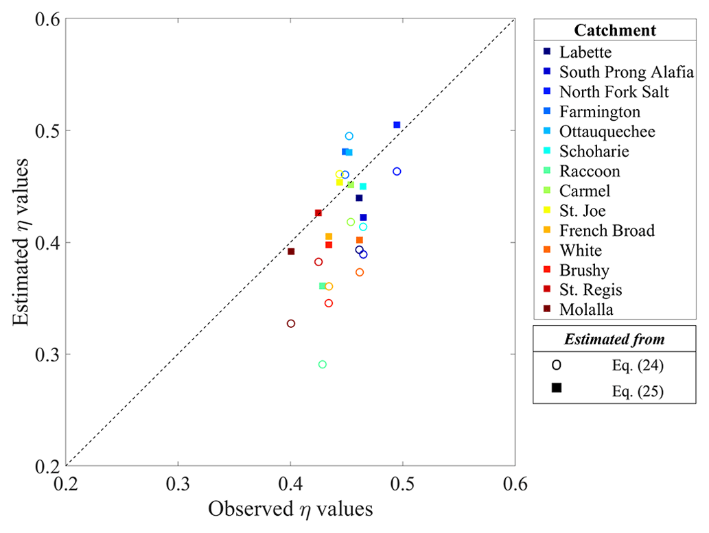
Figure 4 Comparison of η values observed from the ρ_a–A_p relationship (Eq. 18), with η values estimated as the functions of the fractal dimensions expressed as the Horton ratios. Results of Eqs. (24) and (25) are presented as hollow-circle and filled-square markers, respectively. Color codes for our studied river networks are the same as those indicated in Fig. 3.

We perceive the relatively poor performance of Eq. (24) to be the consequence of weak assumptions which form the basis of the theoretical derivations of Eqs. (20) and (23); i.e., Horton's laws hold precisely at all scales of a unit length for measurement (La Barbera and Rosso, 1989; Rosso et al., 1991). Indeed, this assumption is too ideal to be satisfied in real river networks, as corroborated in the non-perfect straight fits when estimating Horton's ratios of our studied networks (Figs. S3 and S4). For D_s, the stream sinuosity cannot be directly analyzed with our DEM analysis due to limited resolution, and so large uncertainty is embedded. As a result, D_s values estimated from Eq. (20) (shown in Table 1) differ from D_s=2 h, with h as seen in Table 1 (Mandelbrot, 1977). With regard to D_b, Phillips (1993), who studied very small catchments in the southern Appalachians in the USA, also demonstrates that satisfying the assumption is necessary to employ Eq. (23).

As shown in Fig. 4, estimated and observed η values are less than 0.5. This can be understood from three perspectives. First, using Eq. (25), 0.5 becomes the upper limit of η, given the physical range of $\mathrm{1}\le D_{\mathrm{b}}\le \mathrm{2}$. Second, the finding of η<0.5 can also be understood from earlier studies on ε, given η=ε. In earlier studies of Eq. (7), ε<0.5 is reported for most river networks (Rodríguez-Iturbe et al., 1992a; Crave and Davy, 1997). Although no attention has been given to the dimensional consistency in Eq. (7), in theory, random critical trees should follow ε≈0.5 (Harris, 1963). Paik and Kumar (2007) investigated trees, ranging from purely deterministic to completely random, and, according to observed ε values, river network organization is based on self-repetitive trees with some randomness in connectivity structure. In their follow-up study, Paik and Kumar (2011) dealt with more scaling laws of river networks to investigate the roles of the connectivity structures in tree organizations. Particularly for Hack's law analysis, they corroborated that partially random trees grounded on deterministic self-repetitive trees only exhibited Hack's exponent h within the range found from river networks.

Lastly, η<0.5 can be explored from the perspective of plausible optimality in the network formation. To explain physical mechanisms resulting in the connectivity pattern of treelike river structures, various optimality hypotheses have been proposed, such as minimizing total energy expenditure (Rodríguez-Iturbe et al., 1992b; Rinaldo et al., 2006), total stream power (Chang, 1979), and total energy dissipation rate (Yang and Song, 1979), as summarized in Paik and Kumar (2010). Although the physical mechanisms are debatable (Paik, 2012), the typical hypotheses share the underlying principle: direct connectivity from individual elements to a common outlet is maximized, while the total length of flow paths is minimized; in turn, there is efficient flow connection in a given space. It is noteworthy that optimal channel networks, which were created in order to achieve the minimum total energy expenditure, showed the satisfaction of Hack's law with h∼0.6 (Ijjasz-Vasquez et al., 1993) and of the area exceedance probability distribution with ε∼0.44 (Bizzi et al., 2018; Carraro et al., 2020). The results suggest that the minimization of total energy expenditure needs to be considered not as a necessary condition but as a sufficient condition. The notion of optimality resides in the quarter-power scaling laws which are linked to Eq. (25). West et al. (1997) suggested “an idealized zeroth-order theory” to explain the emergence of the quarter-power scaling laws in biological systems based on three essential and generic properties of networks in organisms: (1) space filling to serve sufficient resources to everywhere in a system, (2) invariant sizes and characteristics of terminal units, and (3) optimized designs to minimize energy loss. According to their theory (West et al., 1999; West, 2017), the ubiquitous number “4” in the scaling exponent indicates the total number of domains that all metabolic mechanisms operate under through optimized space-filling branching networks, thereby as a sum of the normal three domains representing three-dimensional appearance and the additional one domain revealing fractal dimension feature. Indeed, it is broadly recognized that a river network is an excellent analogue of biological networks in living organisms (Banavar et al., 1999). This implies that the interpretation of the number 4 in the quarter-power scaling laws in biology may help to obtain a mechanism-based insight into the role of the denominator 4 in Eq. (25) for the fractal structures of river networks which have been explained by optimality hypotheses.

5 Summary and conclusions

Thorough investigations of the power-law relationship between the apparent drainage density ρ_a and the pruning area A_p with the exponent of η were conducted. We unraveled the meanings of η with dimensional inconsistencies in diverse aspects. We analytically demonstrated that η is equivalent to the fractal scaling exponent ε in the area exceedance probability distribution based on a hypothetical network following the Hortonian tree framework. This pinpointed the coupled relationship between η and Hack's exponent h that also deviates from the dimensional consistency; i.e., $(\mathit{\eta }=\mathit{\epsilon })+h=\mathrm{1}$.

Our arguments are well supported by evidence from many real river networks, covering wide ranges of climate conditions and free-flowing connectivity levels over the contiguous United States, analyzed with the NHDPlusV2 dataset. The ρ_a–A_p relationships for all studied catchments clearly exhibit curved-head, straight-trunk, and truncated-tail parts, which are identical in shape to the area exceedance probability distributions. Our findings highlighted that the empirical analysis results are in good agreement with the analytically found ones. It suggested that two scaling exponents, η and ε, are fundamentally identical but conceptually distinguishable since geometric and topological attributes are inherent in the calculation procedure for η and ε, respectively. With an analogy of ϵ indicating the compactness of topological hierarchy (Paik and Kumar, 2007), we were able to define the physical meaning of η as the compactness of geometric hierarchy.

Given the scaling-exponent η values for the studied catchments, we identified that these were negatively related to climate conditions represented using the precipitation effectiveness index while not being related to free-flow connectivity levels. The former finding was supported not only by the physical aspect of the hierarchy of river network structures but also by the hydrological mechanisms of the interaction between vegetation and the availability of surface water and groundwater. The latter finding implied that the exponent η might not be linearly controlled by pressures on the capacity of river reaches to flow freely. Both findings provide compelling topics for follow-up research to deeply understand how climate and topography jointly contribute to η and how forcing on free-flow connectivity affects η.

We further examined the physical implications of η based on non-integer fractal dimensions. Such an effort was elaborated upon by expressing η as the functions of fractal dimensions in a single stream and the entire river organization, including the quarter-power scaling relationship. Despite the presence of inevitable uncertainty in quantifying fractal dimensions, the estimated η values were likely to be aligned with the observed ones for all studied rivers. Given that, this study contributed to a deeper understanding of the ρ_a–A_p relationship. Furthermore, our findings lay the foundation for future studies on the interlinkage between fractal dimensions and indicators characterizing self-similar structures of river networks.

Overall, our study sites followed representative scaling laws of river networks despite the differences in climate conditions and connectivity levels. In particular, our findings suggested that the interplay between ε and h for rivers is insensitive to these external conditions. This leads to the natural question of whether the imposed range of external conditions was narrow or whether critical anthropogenic stressors required to uncover exceptional real river networks exhibiting the deviation from the well-known scaling properties were missing. A follow-up study may be needed to resolve such a question, with extended study sites at a global scale and additional descriptors for anthropogenic effects on river network structures and functions.