the Creative Commons Attribution 4.0 License.
the Creative Commons Attribution 4.0 License.
 | 04 Jul 2024
Impacts of climate and land surface change on catchment evapotranspiration and runoff from 1951 to 2020 in Saxony, Germany
Corina Hauffe
This paper addresses the question of how catchment-scale water and energy balances have responded to climatic and land surface changes over the last 70 years in the federal state of Saxony in eastern Germany. Therefore, observational data of hydrological and meteorological monitoring sites from 1951 to 2020 across 71 catchments are examined in a relative water- and energy-partitioning framework to put the recent drought-induced changes into a historical perspective. A comprehensive visualization method is used to analyze the observed time series. The study focuses on changes on a decadal timescale and finds the largest decline in observed runoff in the last decade (2011–2020). The observed decline can be explained by the significant increase in aridity, caused by the reduction in annual mean rainfall and a simultaneous increase in potential evaporation. In a few mainly forested headwater catchments, the observed decline in runoff was even stronger than predicted by climate conditions alone. These catchments are still recovering from past widespread forest damages sustained in the 1970s to 1980s, resulting in a continuous increase in actual evapotranspiration due to forest regrowth. On the contrary, runoff stayed almost constant in other catchments despite an increase in aridity.
These results highlight that water budgets in Saxony are in an unstable, non-stationary regime due to significant climatic changes and the regional impacts of land surface changes such as forest health. The recent decreases in the mean annual runoff are substantial and must be taken into account by the authorities for freshwater management.
- Article
(12654 KB) - Full-text XML
- BibTeX
- EndNote


Annual mean runoff is an important variable in water management as it determines the available freshwater of a catchment. Runoff is governed by climatic conditions which describe the available water based on precipitation; the atmospheric demand for water; and catchment properties such as topography, land cover, soils, and geology (Gentine et al., 2012).
Anthropogenic warming and increasing human pressure on ecosystem services are expected to impact water balance components (Gudmundsson et al., 2021). Recent hydroclimatic trend analysis across Europe shows continental-scale diverging trends for annual mean precipitation, with increases in northern Europe and declines in the Mediterranean region (Masseroni et al., 2021). The signal follows the trend pattern of the wet getting wetter and the dry getting drier, which is driven by global warming (Held and Soden, 2006). Although streamflow trends tend to follow the changes in precipitation, there are regions with diverse trends, with some even opposing the meteorological pattern (Masseroni et al., 2021). Reasons for the diverging patterns in streamflow trends could be manifold: different climatic sensitivities, changes in land surface conditions (Teuling et al., 2019), seasonal changes with earlier snowmelt (Renner and Bernhofer, 2011; Berghuijs et al., 2014), compensating effects, and decadal variability influencing trend analysis (Hannaford et al., 2013). There are also methodological reasons, such as different time windows of available observations.
The eastern part of Germany is such a region where trends in streamflow did not follow trends in climate and where previous research for the federal state of Saxony found large decadal variations, including catchments where major land cover changes occurred that influenced catchment evapotranspiration and runoff (Renner et al., 2014).
Saxony has a long history of hydrological and meteorological observations, which allows hydroclimatic analysis, such as the famous work by Schreiber (1904), who established the first type of Budyko curve, also with data from Saxony. Also, Saxony has a wide range of different topographic characteristics, from the forested Ore Mountains in the south to the flat and arable regions in the northern part. The climate is shaped by the transition of the maritime climate in the west towards a more continental climate in the east. Over the last 70 years, mean annual air temperature rose significantly by about 1.5 K (Franke and Rühle, 2022) due to global warming as a result of anthropogenic greenhouse gas emissions. While greenhouse gas emissions are still increasing, the emissions of sulfur dioxide have been successfully reduced since their peak in the 1980s (Maas and Grennfelt, 2016). Sulfur dioxide has strong environmental impacts. High atmospheric concentrations affect the transmission of visible solar radiation, leading to a reduction in surface solar radiation towards the 1990s and a trend reversal since then (Wild et al., 2005). Air pollution was also the main cause of the tree dieback in the regions of the Ore and Izer mountains (Mazurski, 1986; Šrámek et al., 2008; Maas and Grennfelt, 2016). The forested higher regions were hit more severely since the needleleaf trees comb out fog quite effectively. The fog, which was enriched by sulfuric acid, was intercepted by needleleaf trees and then infiltrated into soils, leading to soil acidification. Over the years, the acidic conditions strongly reduced tree growth and caused widespread tree damages (Pitelka and Raynal, 1989; Maas and Grennfelt, 2016). With the reduction in emissions in the 1990s and reforestation activities, the forests started to regrow (SMUL, 2006; Šrámek et al., 2008). In recent years, forests were also hit by a series of large storms, the 2018–2020 droughts, and a bark beetle bloom. Here especially, monoculture spruce tree forest plantations were hit severely, leading to yet another forest disturbance (Otto et al., 2022).
Renner et al. (2014) analyzed decadal variations in water and energy balance components from 1950 to 2009 and separated the climatic impacts from the land-cover-related impacts on evapotranspiration. They found significant impacts on catchment evapotranspiration as a result of forest disturbance and consistent but not significant impacts as a result of climatic variations. After 2009, climate change continued, and a record-breaking drought occurred in Europe (Rakovec et al., 2022; Büntgen et al., 2021). It becomes natural to ask how runoff responded to this drought and to consider this change in relation to the earlier changes.
This study extends and updates the work of Renner et al. (2014). Therefore, the time series for 71 catchments in the federal state of Saxony are updated and extended to cover the period from 1951 to 2020. The Methods section introduces the coupling of the water and energy balances and explains how this coupling can be used to separate climatic impacts from land cover impacts. Then the dataset is introduced, and in the Results section, the last 70 years are analyzed. The study focuses on the changes from the 2001–2010 decade to the 2011–2020 decade, which actually showed the largest climatic shift observed in this region. The paper closes with a discussion of the impacts of the drought and land cover changes on runoff, as well as potential limitations of the study.
2.1 Catchment water and energy balance
The catchment water balance describes how precipitation P received over the catchment area is partitioned into actual evapotranspiration ET, runoff R at the catchment outlet, and changes in water storage ΔSw:
Precipitation, evapotranspiration, and water storage in soils and groundwater vary spatially, and river discharge integrates runoff processes over the catchment towards the outlet. With the simple water balance equation in Eq. (1), we assume that (i) precipitation which is spatially averaged over the catchment area is the only water input into the catchment and that (ii) runoff observed at the outlet comprises all outflow components. The latter two assumptions require that there are no water fluxes, e.g., by groundwater or water management, across the catchment area (Fan, 2019). When integrating over time, the change in water storage in catchments ΔSw should converge to zero (Dyck and Peschke, 1995), and one can estimate catchment evapotranspiration by . However, having 5–10 years of data is recommended to reduce water storage effects (Zhang et al., 2001).
Evapotranspiration ET is also part of the surface energy balance, here normalized by the latent heat of vaporization L=2.5 MJ kg−1 K−1:
with net radiation Rn, sensible heat H, and an energy storage change term ΔSe. Since available energy, usually expressed as , is not well observed, we assume that it can be described by potential or reference evapotranspiration, denoted as E0 (Choudhury, 1999; Arora, 2002).
ET couples the water and energy balances. As a first consequence of the coupling, we can state that ET is limited by both precipitation and available energy at the same time (Budyko, 1948). Thereby, P and E0 become the two main predictors of the water and energy balance, which is well documented by the Budyko curve (Budyko, 1948). The Budyko curve describes the relative water balance, here , as a function of the aridity index . The semi-empirical functions of Schreiber (1904), Ol'Dekop (1911), Budyko (1948), Pike (1964), and others show good agreement with catchment water budget data from humid to arid climates. The relative water balances of most catchments are close to the physical limits. However, variation in regional catchment properties may affect the partitioning. For example, steep orography or seasonality of precipitation may decrease ET, while the density and type of vegetation, as well as the plant-accessible soil water, tend to increase ET under the same meteorological forcing. These effects were summarized in a catchment parameter from which parametric Budyko curves were developed (Turc, 1961; Mezentsev, 1955; Fu, 1981).
The well-known way to visualize the water and energy coupling is the Budyko plot. The aridity index is plotted on the x axis, and the relative water partitioning is plotted on the y axis. The latter ratio should range between 0 and 1. Low values indicate that most of the rainfall is converted into runoff, and the upper limit of 1 would indicate that all of the received precipitation evaporates.
2.2 Decomposition of climatic and land surface impacts
The second consequence of the complementarity of water and energy balances is that changes in the aridity of a catchment will change not only the relative water balance but also the relative energy balance , only in the opposite direction. This is illustrated in Fig. 1, which plots the relative water balance on the x axis and the relative energy partitioning on the y axis. Any point in the range between 0 and 1 is a reasonable state of the relative water and energy partitioning. The diagonal represents the condition when the aridity index , with humid conditions above and arid conditions below the diagonal line.
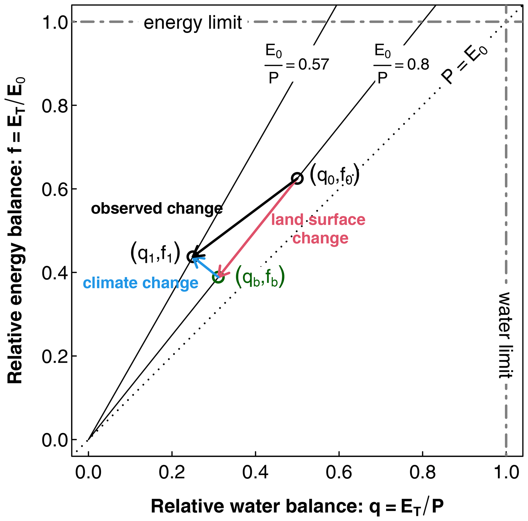
Figure 1Illustration of the separation of climate and land surface changes using a diagram of relative energy to relative water balance. The example shows two hydroclimatic states before (q0, f0) and after (q1, f1) transition. The position of point qb, fb is determined by using the described geometric approach (Eq. 3). The bold arrows depict the climatic and the land surface components of this transition. For illustration, we used case conditions as a reference – P0=1000 mm yr−1, mm yr−1, mm yr−1 – and a state after hypothetical climatic and land surface changes – P1=1400 mm yr−1, mm yr−1, mm yr−1. Thereby, ET decreased by 30 %. The figure is taken from Renner et al. (2014).
The complementarity becomes apparent under a change in aridity. For example, more precipitation will decrease but will increase if the catchment follows a Budyko type of curve. In contrast, if there is solely a change in the catchment attributes without variation in the aridity index, there will be a parallel shift to the line of constant aridity through the origin. An observed change in ET (from point q0, f0 to point q1, f1) can be decomposed into a land surface change part (from point qb, fb to q0, f0 – red arrow in Fig. 1) and a climate change part (from point q1, f1 to qb, fb – blue arrow). Renner et al. (2014) assumed that climatic changes lead to a shift in q and f perpendicularly to the line of constant aridity. With this assumption, the amount of evapotranspiration ET,b without any climatic changes can be computed from data before (index 0) and after the change (index 1):
Then the climate-induced change in evapotranspiration can be calculated by , and the remaining part can be denoted as the land-surface-induced change ; see Renner et al. (2014) and Sect. B1 for a detailed derivation.
By applying the water budget equation to the changes, i.e., , we can also compute the amount of runoff change attributed to climatic changes:
where R1 is the mean annual runoff in the second period, and P0 is the mean annual precipitation of the first period. The land-surface-induced changes in runoff are derived by
where R0 is the mean annual runoff of the first period. Note that changes in runoff are mainly driven by changes in precipitation (Dooge, 1992) and secondly by changes in evaporative demand and land surface conditions.
Other approaches to decompose climate and land surface impacts on runoff were proposed by Wang and Hejazi (2011), Jaramillo et al. (2013), and Jaramillo and Destouni (2015). These methods use Budyko functions to estimate the climatic change part. However, the uncertainties in quantifying catchment precipitation, runoff, and energy demand are more relevant than the methodological differences.
2.3 Comprehensive visualization method
The decadal changes in catchment evapotranspiration are related to precipitation and potential evapotranspiration and are plotted together in the joint water energy balance diagram. This allows a visual interpretation of separate climatic and land surface impacts on catchment evapotranspiration, as illustrated in Fig. 1. Therefore, decadal averages of the relative water () and energy () partitioning for each of the 71 catchments are calculated. Subsequently, the decadal averages of both ratios for a given decade and each catchment are plotted in the joint water energy balance diagram. The position of a catchment within the plot is depicted as a pie chart. This holds information about the land use types (see Sect. 3.3) of each catchment.
The change in the relative water () and energy () partitioning towards the following decade is integrated as an arrow. The direction of the arrow reveals if only climatic or land surface changes occurred or if both types of changes were present. The arrow length refers to the magnitude of the change. In order to assess if a change is statistically significant, a two-sample Hotelling's T2 test (Todorov and Filzmoser, 2009) is performed by sampling the annual data of each decade. Bold black arrows highlight if the magnitude of a change in the decadal mean between 2 decades is larger than the year-to-year variability using a significance level of α=0.1. Thin gray arrows visualize the direction of an insignificant change.
Furthermore, a map is added with the outline of the analyzed Saxonian catchments to illustrate where the changes occurred. The arrows are also included in the map and start at the river gauge location. This is combined with spatial information of forest damage data (see Sect. 3.3).
If several of these comprehensive visualization diagrams are plotted as a sequence over a number of decades, this provides information about temporal, as well as spatial, changes in the catchment water balance. It allows the identification of general behavior within a large catchment sample and may also reveal differences for certain catchment groups. At the same time, the analysis of probable causes is possible.
In this section, details about the used datasets for the hydroclimatological analysis are provided. Note that this study updates the analysis presented by Renner et al. (2014) by adding data from 2010 to 2020. Thereby, the same catchments and methods are used as in Renner et al. (2014). However, the hydrological and meteorological input data were updated, containing data corrections and additional meteorological data due to digitization efforts.
3.1 Hydrological data
The study covers data of 71 river gauging stations with long-term, high-quality data records. The sites where chosen according to continuity, homogeneity, and/or small direct impacts by water management due to dam operations or large mining activities such as in the Lausitz region in the east of Saxony. The sampling of the catchments thus slightly over-represents the higher regions of Saxony. It is also important to note that the sample includes nested catchments, which share parts of the catchment area and are thus not independent. All catchment attribute data such as river names and catchment polygons were taken from Renner et al. (2014). The map in Fig. 2 provides an overview. All time series data were updated. The key data provider is the Saxon State Department for Environment, Agriculture and Geology (Landesamt für Umwelt, Landwirtschaft und Geologie, LfULG), which provided daily runoff time series data via the web portal (https://www.umwelt.sachsen.de/umwelt/infosysteme/ida/index.xhtml, last access: 12 March 2023) and by email. The river gauge Greiz/Weiße Elster is operated by the Thuringian State Department of Environment, Mining and Nature Conservation (TLUBN), and time series data were obtained directly from the authority. All data were checked graphically for correctness. Data screening for homogeneity and dominant influences like water management was performed in Renner et al. (2014), and such catchments were removed from the dataset. This was necessary because we employ the simple water balance equation (Eq. 1) to estimate ET.
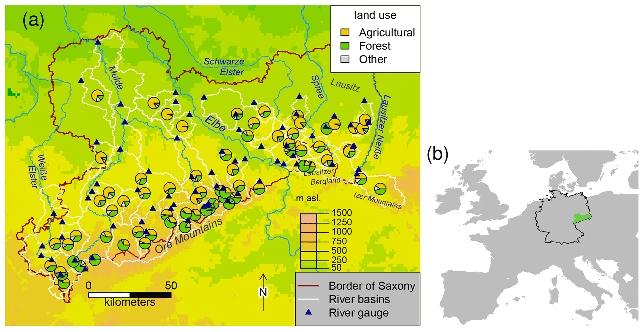
Figure 2(a) Map of the federal state of Saxony and its topography, catchment boundaries, and river discharge measurement stations analyzed in this study. The land use fraction depicted as a pie chart of each catchment is derived from CORINE land cover data from the year 2000. Panel (b) shows the location of Saxony, with Germany and Europe for orientation, using polygon data from NUTS 2021 (https://commission.europa.eu/index_de, last access: 1 September 2023). The figure is adapted from Renner et al. (2014).
At first, daily discharge data were aggregated to monthly averages with at least 20 non-missing values per month. Then annual averages were computed using the hydrological year from November to October. Finally, decadal averages and statistics were derived when at least 6 years of complete data per decade were available. Runoff yield (mm yr−1) was calculated from average discharge records (m3 s−1) by multiplying with the number of seconds per year and dividing by the catchment area.
The study period covers 1951–2020. For computing the long-term average runoff, all available annual data per site were used. Note that not all runoff time series cover the whole period. In a few catchments, river gauge relocation occurred, leading to a change in the station ID. At the following sites, the time series of the prior gauge and the current station were merged for this study: Buschmühle/Kirnitzsch, Piskowitz 2/Ketzerbach, and Annaberg/Sehma. Table A1 provides an overview of the river gauges and the time series availability.
3.2 Meteorological data
Precipitation and potential evaporation were derived from meteorological station data and were interpolated on a spatial grid, from which catchment averages were extracted. Precipitation is well observed in the study area, with 845 sites used in the regionalization and 366 sites with more than 40 years of data, shown as circles in Fig. 3a. The size of the circles reflects the available observation years. Key operators are the German weather service, the Landestalsperrenverwaltung Sachsen (river dam authority of the federal state of Saxony), and the Czech and Polish hydrometeorological institutes. All meteorological station data were acquired at daily resolution from the REKIS (http://rekis.org, last access: 9 February 2022) data service, which is a platform for regional meteorological data services covering the federal states of Saxony, Thuringia, and Saxony-Anhalt.
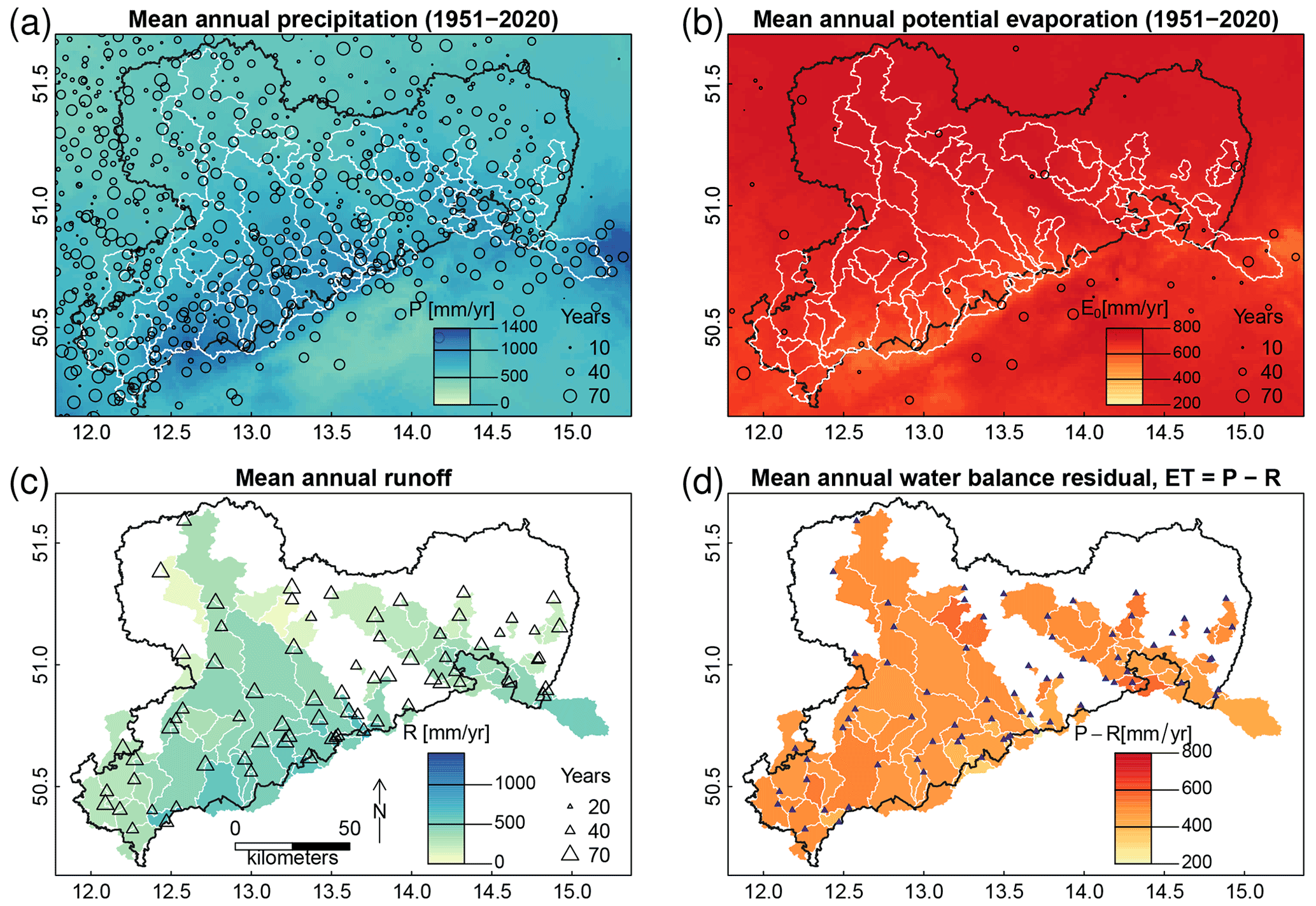
Figure 3Maps of long-term (1951–2020) annual mean (a) precipitation, (b) annual potential evapotranspiration (FAO-56 grass reference evapotranspiration; Allen et al., 1994), (c) annual runoff, and (d) residual water budgets (). Observation stations which have been used to derive spatial fields of P and E0 are depicted as circles with diameters corresponding to the number of years of available data. The maps of mean annual precipitation P and the FAO reference potential evapotranspiration E0 have been derived by averaging the individual annual raster maps used to calculate the basin averages. Note that panels (a) and (c) and panels (b) and (d) use the same color scale, respectively.
The original daily precipitation data were added up to annual totals using the hydrological year from November to October. The annual station data were then interpolated on a 1.5 km grid using an automatic universal Kriging procedure provided with R package automap (Hiemstra et al., 2009). Thereby, station altitude is used as the dependent variable. The procedure was validated by Renner and Bernhofer (2011) and Renner et al. (2014).
To model potential evaporation (E0), we use the FAO-56 method for grass reference evapotranspiration (Allen et al., 1994). This is a simplification of the Penman–Monteith equation, and Allen et al. (1994) provide methods to substitute net radiation data and ground heat flux, which are not commonly available. Here, the daily station data were first aggregated to monthly averages to compute E0 from temperature (daily mean, minimum, maximum), sunshine duration, relative humidity, and wind speed data. The locations of the 115 climate stations (40 sites have more than 40 years of data) are shown as circles in Fig. 3b. Similarly to precipitation, spatial interpolation was performed on available annual (hydrological year) station data and interpolated onto a 1.5 km grid using the universal Kriging procedure with altitude as the dependent variable.
3.3 Land use and forest damage data
The remote-sensing-based CORINE land cover dataset (© European Union, Copernicus Land Monitoring Service, European Environment Agency – EEA) was used for land use classification of the catchments and as a proxy for forest damage. Snapshots for different years are available.
From the CORINE snapshot of the year 2000, we classified the land use types of forested and near-natural vegetation as “forest”; merged all agricultural and grass lands into the class “agricultural”; and grouped the remaining types, mainly built-up areas, as “others”. The first CORINE snapshot from the year 1990 was used to estimate the relative area of forest damage per catchment, following Renner et al. (2014). The CORINE land cover class transitional scrub forest (324) includes areas of damaged forests (Bossard et al., 2000). This snapshot of 1990 captures the period of maximal forest damage extent in central Europe. Based on these data, Renner et al. (2014) calculated the relative affected area for each catchment and classified the catchments into groups with different magnitudes of forest damage. The class of major forest damages, with a threshold of >20 % of catchment area, was selected following Bosch and Hewlett (1982), who reported significant streamflow increases in paired catchment studies after clear-cuts when more than 20 % of the catchment area was affected. The threshold category of 2 %–20 % was applied to select catchments where a measurable area was affected. Renner et al. (2014) found that 38 % of the catchments have no forest damage (<0.01 %), 21 % have minorly affected areas (0.01 %–2 %), 31 % have considerably damaged areas (2 %–20 %), and 10 % of the catchments have damaged areas larger than 20 %. These catchments are shown in the map in Fig. 4.
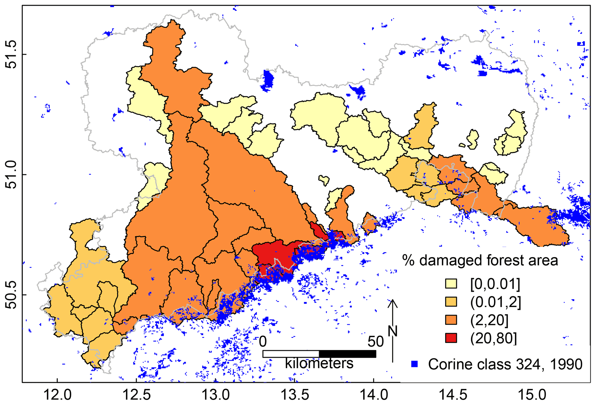
Figure 4Map of forest damage using CORINE 1990 class 324 (transitional scrub forest). Catchments are grouped by the relative area of forest damage.
In order to get an idea of the forest damage over time, we also used the CORINE snapshots of the years 2000 and 2012. For the pre-satellite era, maps of canopy damage data available for the years 1960, 1970, 1980, and 1990 were used. Canopy damage was assessed by needle and leaf losses in the canopy (SMUL, 2006) and follows a measurement protocol defined in the former German Democratic Republic (Forstprojektierung, 1970).
4.1 Long-term hydroclimatology of Saxony
In this section, the long-term average (1951–2020) hydroclimatology of Saxony is illustrated based on the established dataset; see also Table A1.
Annual average precipitation is 830 mm yr−1 across the 71 catchments and ranges between 607 and 1151 mm yr−1. For the whole of Saxony, an average of 712 mm yr−1 is estimated. The difference is due to the sampling of the catchments, which over-represents higher regions of Saxony. Precipitation shows a distinct north-to-south increasing gradient which is linked to altitude. Another, although weaker, gradient is induced by the transition of maritime to continental climate, which results in decreased precipitation from west to east (Figs. 3a and 5a).
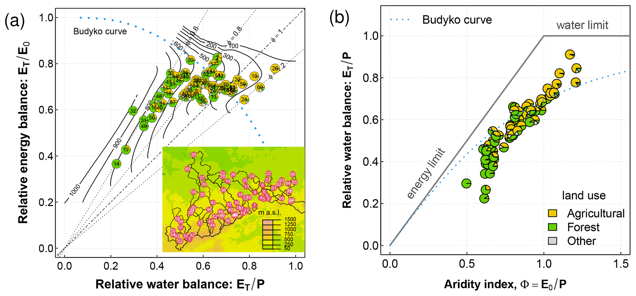
Figure 5Long-term catchment water and energy partitioning of the catchments. Panel (a) plots the relative energy vs. water balance. The average basin elevation is used to predict the contour lines using local polynomial (LOESS) regression. This demonstrates the general height dependency of the catchments' climate and land use (CORINE dataset of 2000), as well as the transition from wet basins with high runoff ratios to lower values. The inset in panel (a) shows a map of the catchments, as well as their gauge ID numbers and altitudes as background rasters. Panel (b) visualizes the same data but in the classic Budyko diagram with relative water balance vs. aridity index. The catchments are depicted as pie charts which show the areal percentage of land use of each catchment.
The FAO grass reference potential evapotranspiration E0 across the study catchments ranges between 572 and 738 mm yr−1 and is on average 669 mm yr−1. E0 is negatively correlated with elevation (see Fig. 3b).
The spatial pattern of runoff is dominated by topography and precipitation, with most catchments receiving a large amount of their water from the headwater catchments in the Ore Mountains, the Lausitzer Bergland, and the Izer Mountains; see Fig. 3c. The lowest annual runoff values are found in the lowland catchments in the north (minimum 59 mm yr−1), and the highest values are found in the headwater catchments in the south (maximum 799 mm yr−1). On average, runoff is 372 mm yr−1 across the 71 catchments.
The difference of P−R is used to estimate actual catchment evapotranspiration ET (Fig. 3d). ET is, on average, 461 mm yr−1 for all catchments and is 572 mm yr−1 at its maximum. The lowest values of annual ET are found in the high headwater basins (minimum 219 mm yr−1). In general, ET has a smaller spatial variation than runoff. All long-term average data are summarized in detail in Table A1.
The average water and energy partitionings of the catchments in Saxony are illustrated in Fig. 5a and b, which show the relative water–energy partitioning diagram and the Budyko plot, respectively. Each catchment is depicted as a pie chart, representing the relative portion of forested and agricultural area. Furthermore, contour lines are included in Fig. 5a, derived from the mean catchment altitude.
The relative water partitioning is placed on the x axis in Fig. 5a and on the y axis in Fig. 5b. The long-term averages of vary between 0.22 and 0.91 and are on average 0.57.
On the y axis of Fig. 5a, the relative energy partitioning is plotted, also ranging between 0 and 1. This ratio varies between 0.37 and 0.83, with most catchments clustering around the average value of . Plotting both ratios together combines the two key meteorological forcing variables P and E0. Four general examples for the aridity index are included in Fig. 5a as lines through the origin. When precipitation equals potential evaporation P=E0, this would fall on the diagonal. More humid conditions would be above the diagonal of ϕ=1, while more arid conditions fall below this diagonal. All together, catchments at higher altitudes (see altitude contour lines in Fig. 5a) are more humid, with , and have a larger portion of forested area. Catchments with are generally found at lower altitudes and are dominated by agricultural land use.
The aridity index ϕ is also visualized on the x axis in the Budyko plot (see Fig. 5b) and ranges between 0.50 at the highest catchment and 1.21 at the lowest catchment. On average, we find a value of . The Budyko function (Budyko, 1948) is plotted as a reference, allowing the prediction of catchment ET from the aridity index. The distribution of the data generally agrees with the Budyko function. However, there is an overestimation of in the more humid catchments and an underestimation in the drier catchments.
4.2 Annual and decadal dynamics in joint water and energy balance
4.2.1 Variability of meteorological forcing
The variability of the meteorological forcings P and E0 will be analyzed using the annual mean values, as well as the decadal means (see Fig. 6). Generally, there is a larger variability in precipitation P, both across catchments and from year to year, than in E0. The decadal mean precipitation over all basins was always higher than E0. However, the last decade (2011–2020) shows a remarkable increase in E0, being the highest decadal average so far (710 mm yr−1) and getting closer to P (814 mm yr−1). At an annual timescale, about 17 % of the years had a negative climatic water balance, where the catchment annual average E0 was larger than P: 1951, 1953, 1959, 1963, 1964, 1976, 1982, 1990, 1991, 2003, 2015, and 2018. The occurrence of these negative values does not have a clear trend but indicates that there have already been dry conditions in the 1950s and 1960s.
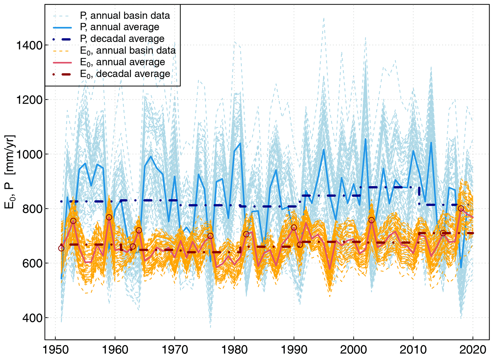
Figure 6Time series of annual P and E0 for all basins (thin dashed lines), cross-basin annual average time series (full lines), and all basin decadal averages (dot-dashed lines).
4.2.2 Variability of catchment evapotranspiration
The water budget residual P−R is analyzed as proxy for basin-scale ET, which may include the unknown influence of past water storage changes ΔSw. To reduce the effect of storage changes, decadal averages of ET are derived, as presented in Fig. 7. In the figure, catchments are grouped by the percentage of areal forest damage extent, as shown in Fig. 4.
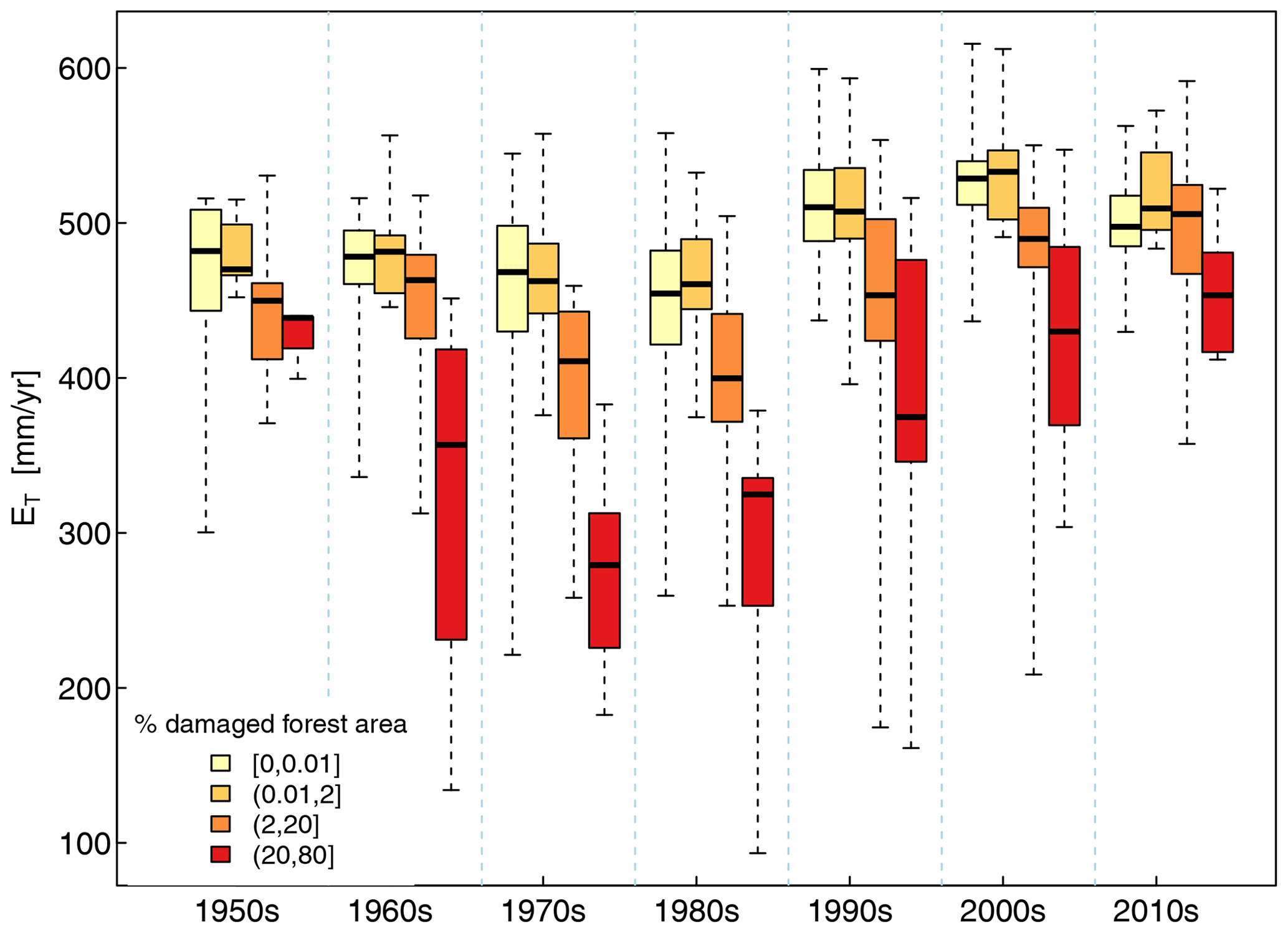
Figure 7Boxplots of decadal averages of ET for four groups of catchments with different ranges of damaged forest area per catchment area using the CORINE 1990 class 324 (transitional scrub forest).
The boxplots in Fig. 7 depict variations in the decadal average of ET for all catchments in each group. During the first decade, 1951–1960, there is no large difference between these four groups. Between 1961–1980, the heavily damaged group experienced a large decline in ET, while the two groups with low damage effects show little variation. The catchments with moderately damaged forest are in between and show a minor decrease in ET during the decades from 1971 to 1990. From 1991 to 2010, the effect is reversed for all catchments with moderately and heavily damaged forest, and this is reflected in a pronounced increase in ET (see Fig. 7). Additionally, while the positive trend in ET continues for the group with considerable forest damages, the lowly damaged catchments show a small but consistent decline during the last decade.
4.3 Decomposition of climate and land surface effects
The changes in runoff are decomposed in climate and land surface change components, which together sum up to the observed change. The decomposition method by Renner et al. (2014), introduced in the Methods section, quantifies the contributions of climatic changes in P and E0, as well as land surface changes in ET, in retrospect. Figure 8 presents the results of the decomposition for catchment runoff. The gray boxplots depict the changes in the observed runoff from one decade to the next for all the catchments. There is not much variation in the median of the changes from 1951 to 2010 and no clear tendency for the direction of change. The observed changes in runoff varied between −50 and 50 mm yr−1 across the Saxonian catchments. In the last decade, observed runoff decreased the most across the majority of catchments, with a median decline of −70 mm yr−1, which is 8 % of the mean annual precipitation.
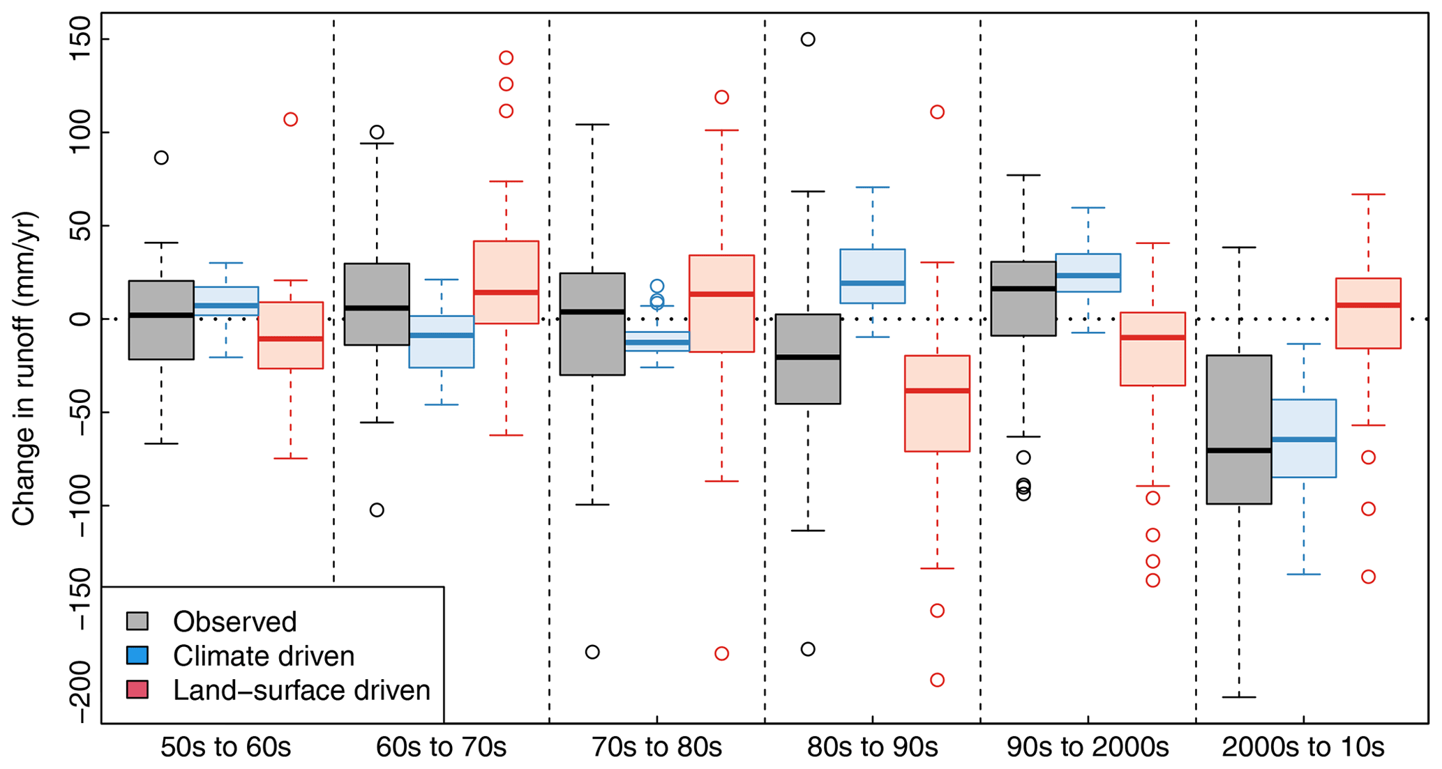
Figure 8Decadal changes in annual mean catchment runoff across all catchments. Box whisker plots are shown for observed (gray), climate (blue), and land surface attributed runoff changes using the decomposition method introduced in the Methods section. The boxes show the interquartile range (IQR), with the bold horizontal line being the median of the distribution. The whiskers show the outer ranges, with points marking outliers outside a 1.5 IQR range.
The decomposition quantifies the contributions of climatic changes in P and E0 to runoff, visualized as blue boxplots in Fig. 8. Thereby, the climatically driven runoff changes were relatively small in the first five transitions, with median changes between −13 mm yr−1 towards the 1980s and +23 mm yr−1 towards the 2000s. The climate-driven changes became the dominant cause in the last transition, with a median change of −65 mm yr−1, explaining the observed decline in runoff in most catchments in Saxony. However, note that the transitions from the 1980s to the 1990s and from the 1990s to the 2000s showed two consecutive increases in the climatic runoff change component due to increases in precipitation.
The red boxplots in Fig. 8 represent the land surface change component. The outliers show that, in a few catchments, it dominated the change in runoff during the past decades. There have been two consecutive but small increases of 14 mm yr−1 in runoff due to land surface conditions towards the 1970s and 1980s. They were followed by a strong and more widespread decline in the 1990s, with a median decrease of −38 mm yr−1 in the land surface component.
4.4 Decadal dynamics of water–energy partitioning from 1951 to 2000
The decadal changes within the 70-year period are depicted by six panels in Fig. 9. In each panel, the changes in the water- and energy-partitioning ratios from one decade to the next are visualized by the direction and length of the arrows. The displayed pie charts always refer to the same land use types derived from the CORINE dataset of the year 2000. The number of catchments taken into account varies due to the different availability of data.
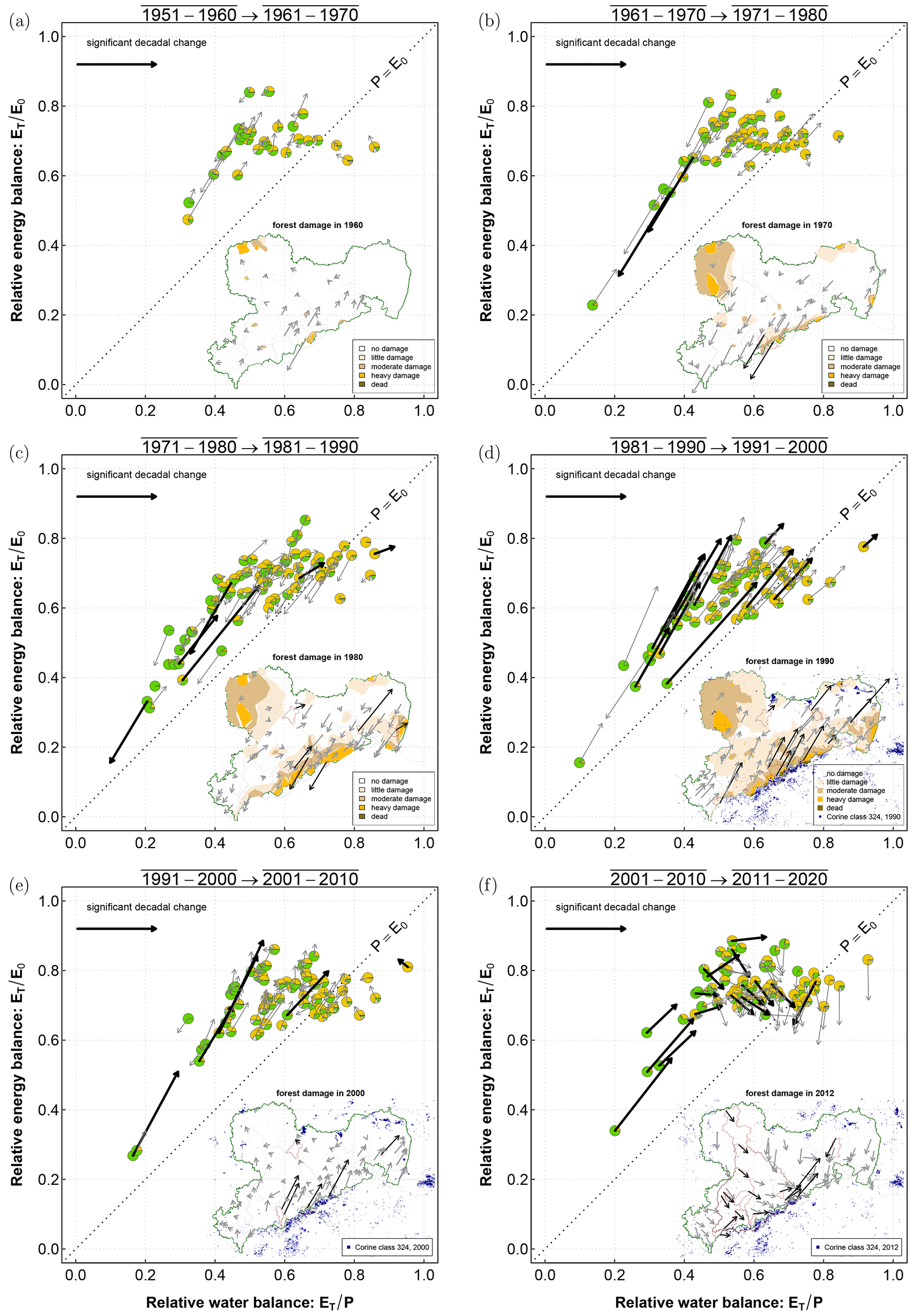
Figure 9Annual averages per decade of the water- and energy-partitioning ratios for each basin analyzed. The arrows denote the change from one decade into the following decade. There is one panel for each decadal change, starting in the 1950s in panel (a) and moving to the 2000s and the 2010s in panel (f). Significant changes are marked with bold arrows and a red border of the respective catchment in the map inset. The inlay maps show the location of the river gauges and the spatial extent of forest damages, and from 1990, blue pixels show the CORINE transitional forest class.
Figure 9a shows a set of 28 catchments in the decade 1951–1960 with a transition into the next decade. No significant changes in and are apparent. In Fig. 9b, the transition from the 1960s to the 1970s is visualized. The number of available catchments increases to 45. The changes within the catchments are pointing either towards the origin of the diagram or in the opposite direction, but these are not significant for most of the catchments. Only two neighboring headwater catchments in the upper Ore Mountains (Rothenthal/Natschung and Zöblitz/Schwarze Pockau) have significant decreases in both ratios, indicating an impact of land surface changes on ET. Also, other neighboring catchments show decreases, which hints at a similar cause. These declines in ET are mostly in the more humid headwater catchments and are part of the group with dominant forest damage, as presented in Fig. 7.
The extent and severity of forest damages increased in the 1980s; see the inlay maps of forest damage in Fig. 9c). The transition from the 1970s to the 1980s was analyzed for 69 catchments and can be seen in Fig. 9c). The development of the two ratios appears to be dominated by this ongoing spread of forest damages, with many of the arrows showing the directions of land surface changes. For two catchments in the upper Ore Mountains (Rehefeld/Wilde Weisseritz and Wolfsgrund/Chemnitzbach), the declines in and are significant, while four catchments experience a significant increase in the two ratios.
In contrast to the prior transitions, the changes are almost consistent for all of the catchments in the transition from the 1980s to the 1990s depicted in Fig. 9d. The transition from the 1980s to the 1990s reveals the most drastic and coherent shifts observed in the whole period, with dominant and significant increases in both ratios in 11 out of 69 catchments. For some of the catchments, this even means a reversed direction of the changes for and compared to earlier periods. In 1990, forest damage reached its largest extent in Saxony. In addition, increases in precipitation and potential evaporation led to a further increase in catchment evapotranspiration; see Fig. 6. The following decadal change from 1991–2000 to 2001–2010 is visualized in Fig. 9e. Now there are two groups with a different development in terms of the water and energy partitioning. While the mountainous catchments, which were highly effected by the vast forest damages, still have a continuing increase in and , the lower-lying regions generally show fewer changes with no clear direction. Figure 9e also reveals five mountainous catchments with significant recoveries of both ratios. On the contrary, the lowland catchment Seerhausen/Jahna has a significant decrease in its aridity index due to higher precipitation.
In general, the land-surface-attributed impacts were dominant in the development of the two ratios and for the time period between 1951 and 2010. This analysis was part of the previous work of Renner et al. (2014). The picture changes when it comes to the transition from 2001–2010 to the last fully observed decade of 2011–2020, which is presented in the next section.
4.5 Decadal dynamics of water–energy partitioning from the 2000s to the 2010s
The last decadal transition is dominated by the meteorological conditions of 2011–2020, which have been much drier than the 2 decades before. This results in the highest number of significant changes (16 out of 64, 25 %) in catchment water and energy partitioning, as presented in Fig. 9f. The direction of change is now mainly orthogonal to the prior transitions, meaning that climate-attributed impacts affect the ratios of and the most.
Two more figures are included to illustrate the noticeable changing conditions from 2001–2010 to 2011–2020 in Saxony. Figure 10 visualizes the decadal changes as bar plots for all analyzed water balance components and all 71 catchments. The reduction in precipitation (blue bars in Fig. 10), on the one hand, and the uptake in the potential evaporation (red bars in Fig. 10), on the other hand, are apparent. The widespread and large decline in annual precipitation resulted in a median decrease of −59 mm yr−1. It was rather pronounced in the Ore Mountains, reaching up to −143 mm yr−1, and the Izer Mountains, which feed the upper Lausitzer Neiße River; see Fig. 11a. The maps in Fig. 11a combine precipitation changes (filled polygons of the catchment area) with changes in observed runoff (filled triangles at the river gauge locations). The same color scale is used to highlight how much the regional precipitation decreases affected runoff. This combination shows that catchment runoff broadly followed precipitation. In 56 out of 64 catchments, the observed runoff decreased, with a median decline of −73 mm yr−1.
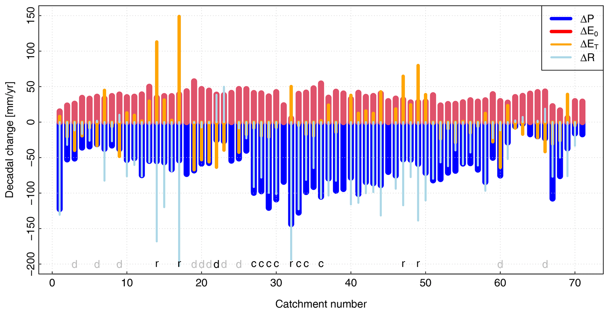
Figure 10Change in decadal water balance components from the decade 2001–2010 to the decade 2011–2020 (in mm yr−1) for each catchment.
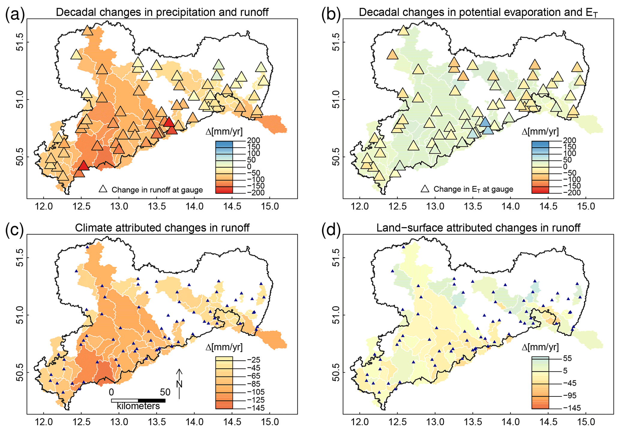
Figure 11Maps of decadal changes (2001–2010 to 2011–2020) in (a) precipitation and runoff, (b) potential evaporation (FAO-56 grass reference evapotranspiration; Allen et al., 1994) and catchment evapotranspiration (), (c) climate-attributed changes in runoff, and (d) land-surface-attributed changes in runoff. While panels (a) and (b) visualize the changes on the catchment level and at the gauging stations (triangles), panels (c) and (d) use only the catchment area to present changes.
Focusing on the significant changes, three different types can be observed: (i) five catchments in the Ore Mountains show continuing recovery effects, with significant increases in both ratios, as marked by the letter “r” in Fig. 10. These catchments have had large areal extents of forest damages, the recovery from which led to catchment evapotranspiration rates now being even higher than during the 1951–1960 decade, as can be seen in Fig. 7. Type (ii) constitutes catchments, especially in the Mulde River basin, which experienced notably significant decreases in annual mean precipitation. Nine of the catchments show significant movements in the climatic-change direction, marked by the letter “c” in Fig. 10. These catchments follow the Budyko curve and retain high evapotranspiration, leading to increases in the relative water balance. Type (iii) constitutes the lowland catchments in northern and eastern Saxony, recognizable by the downward-pointing arrows in Fig. 9f and marked by the letter “d” in Fig. 10. These represent a decrease in the relative energy partitioning without a change in the relative water balance. Only one catchment (Zescha/Hoyerswerdaer Schwarzwasser) experienced a significant change. Here, the increase in potential evaporation did not lead to an increase in catchment evapotranspiration. This highlights that both climate changes (i.e., higher aridity) and land surface changes co-occurred in this transition period. A similar behavior was also found by Pluntke et al. (2023) for a small, forested research catchment in the south of Dresden, Saxony.
The map in Fig. 11a also highlights notable exceptions: (i) there are a few catchments in the upper Ore Mountains with larger decreases in runoff than in precipitation, and (ii) four catchments located in the east of Saxony have notable increases in runoff despite increasing aridity.
In addition to lower precipitation amounts, there was a substantial increase in FAO reference potential evaporation across all regions, with a median increase of 36 mm yr−1; see the red bars in Fig. 10. The map in Fig. 11b presents a rather uniform spatial distribution of the change in potential evapotranspiration, with slightly larger increases in lower parts of Saxony. In this map, the changes in actual catchment evapotranspiration ET (derived from P−R) are added with the same color scale. The response of actual evapotranspiration is rather mixed. A total of 27 out of 64 catchments depict a reduced ET, with −10 to −67 mm yr−1; see also the orange bars in Fig. 10. These catchments are found in the lower regions of Saxony. In particular, the smaller tributaries to the Elbe River and the catchments in the Lausitz show these reductions (triangles in Fig. 11b). Furthermore, 16 catchments experienced increases in ET larger than 10 mm yr−1. In five of these catchments in the upper mountain regions, the increase even exceeded 50 mm yr−1. The remaining 21 catchments have only smaller changes in ET.
The already-discussed decomposition method was applied to quantify the climatic and the land surface impact on runoff changes. The climatic impact of the observed changes in precipitation and potential evaporation on runoff is visualized in the map in Fig. 11c. The catchments in the Mulde River basin show the largest decreases in the middle of Saxony, and there are also larger effects seen in the upper Lausitzer Neiße River basin. Note that these catchments have a more humid climate and higher runoff ratios, which generally lead to a higher sensitivity of absolute runoff amount to changes in precipitation (Dooge, 1992; Renner et al., 2012). In the decade of 2011–2020, the increasing dryness had the strongest climate impact on runoff in Saxony in the whole period analyzed here (see Fig. 8).
Figure 11d shows the spatial distribution of the land surface impacts on runoff. Many catchments reveal only minor effects of land surface changes. However, there are interesting exceptions. The group of catchments with the large increases in ET and corresponding pronounced declines in runoff is the one with the most land surface impacts. The catchments are all located in forested regions, where the recovery of past forest damages is still ongoing (Ore Mountains, the Lausitzer Bergland), as presented in Fig. 11d. There are also catchments with increasing runoff attributed to land surface impacts, as shown in Fig. 11d. These are predominantly lowland catchments with higher aridity indices and no decrease in runoff, as expected from the climatic conditions, resulting in downward arrows in Fig. 9f. The discussion of the potential causes is left for the next section.
In this study, we identified and estimated the impacts of climate and land surface conditions on catchment water balance in the federal state of Saxony. First, we discuss the attributed climatic and land cover impacts on catchment water balance, and then we close with an explanation of the potential limitations of the study.
5.1 Climate change becomes a significant driver of water balance
The drought from 2018 to 2020 in Europe was exceptional in terms of spatial extent, duration, and intensity (Rakovec et al., 2022; Büntgen et al., 2021). Compared to previous drought events, it was exceptionally warm (Rakovec et al., 2022) and was probably caused by anthropogenic warming (Büntgen et al., 2021). The drought assessment of Rakovec et al. (2022) used a modeled soil moisture index based on meteorological data reconstructions from 1766 to 2020 for Europe. According to Rakovec et al. (2022), northern Saxony and the Lausitz region exhibit a soil moisture drought of 24 months. Low-flow statistics showed long durations of hydrological drought conditions, which were also exceptionally low in Saxony. The Saxon State Department of Environment, Agriculture and Geology reported that, during the summertime of 2018–2019 and 2020, 40 % to 70 % of 146 runoff gauges in Saxony showed values below the mean annual low flow (Franke and Rühle, 2022). Due to the long duration, mean annual flows of 2018–2020 were also lower than the long-term mean (Franke and Rühle, 2022).
The widespread runoff decline in Saxony represents the largest and most coherent decadal shift in runoff, and the decomposition methods highlight that this reduction is caused by climatic changes – that is, the reduction in rainfall and the increase in atmospheric demand for water (see Figs. 6 to 8). For the majority of catchments, the reduction in runoff can thus be predicted by knowing the changes in annual mean precipitation and potential evaporation. However, there were notable exceptions in certain regions, which are discussed next.
5.2 Land surface impacts on water and energy partitioning
Any change in runoff which cannot be predicted with the climatic signal is attributed to land surface changes. In the last decade, with the shift towards more arid conditions, we observed two different reactions in catchment runoff, which were attributed to land surface impacts. While some catchments showed stable or even increasing runoff, others experienced very strong declines in runoff which could not be explained by the dryness; see Sect. 4.5.
5.2.1 Hydrological response to forest recovery under dry conditions
Large-scale forest dieback due to the effects of air pollution occurred in central Europe with the industrial use of lignite coal burning, with significant regional impacts starting in the 1960s (Mazurski, 1986; Maas and Grennfelt, 2016). Renner et al. (2014) documented, on the one hand, that these forest damages led to strong reductions in catchment actual evapotranspiration lasting over 2 to 3 decades and, on the other hand, that an increase in ET correlates with the recovery of forests. This link between forest damage and substantial declines in catchment evapotranspiration is updated in this study and is clearly revealed by decadal averages of ET (see Fig. 7). The effect becomes apparent when the catchments are grouped by the percentage of forest damage.
Since 1990, the recovery of these areas led to increases in catchment evapotranspiration and reduced the gap between disturbed and undisturbed catchments in Saxony. Nevertheless, the analysis of climatic and land-surface-attributed changes in relation to runoff, visualized in Figs. 9f and 11d, points out that, in a few mountainous catchments, the recovery of ET is still ongoing. The largest increases were seen in the eastern Ore Mountains at the neighboring catchments Baerenfels/Pöbelbach and Rehefeld/Wilde Weißeritz, followed by the middle Ore Mountains (Rauschenbach/Rauschenfluß and Deutschgeorgenthal/Rauschenbach) and a headwater catchment in the western Ore Mountains (Sachsengrund/Große Pyra). At these catchments, the strong increases in ET correlate to exceptional decreases in annual mean runoff. Hereby, it is noticeable that the change in runoff is larger than the observed decrease in precipitation. Furthermore, the increase in ET is higher than in E0 (see Fig. 10). This strongly hints at the recovery of transpiration and evaporation from interception due to vegetation regrowth. The long-term time series of catchment evapotranspiration presented in Fig. 7 shows that the recovery in terms of ET in these catchments is almost completed. On the one hand, the magnitude of ET is now at the same level or is even higher than prior to the period of large-scale forest damages. On the other hand, ET is now in a similar range compared to catchments without severe forest damages.
5.2.2 Potential causes of constant or increasing runoff
At first sight, it seems contradictory that runoff remained stable or increased even though precipitation decreased and potential evaporation increased. A potential hypothesis explaining this behavior may be the reduced transpiration and evaporation from interception due to reduced growth or plant damage. This hypothesis is supported by forest inventory data from Saxony (Otto et al., 2022) showing that, by far, the largest amount of damaged wood due to bark beetle infestations occurred in 2018–2020 within more than 70 years of observations. The combination of warm and dry conditions reduced the fitness of needleleaf trees, which then led to an outbreak of bark beetles in 2018 that continued until 2020 throughout Saxony. Thereby, the forests in eastern Saxony were most affected, which is in line with regions where we observed stable or increasing runoff conditions and thus decreases in catchment actual evapotranspiration (see Fig. 11).
Apart from forests, there is evidence of reduced crop yields during the drought year 2018 (Statistisches Landesamt Freistaat Sachsen, 2022). This year showed the highest aridity index in the analyzed period. The reduction in yields corresponds to the depletion of soil moisture during the long and severe drought, especially in northern and eastern Saxony (Rakovec et al., 2022). Water limitation causes reduced plant growth, as well as reduced transpiration via stomata closure (Teuling et al., 2010). However, more research is required to quantify the contribution of reduced transpiration of short vegetation such as grass and crops to reduced catchment evapotranspiration. In either case, a future recovery of vegetation, especially of forests, will likely increase ET and thus lead to less runoff from such catchments if precipitation remains low.
An alternative hypothesis for the stable runoff under increasing aridity could be the contribution of groundwater release as baseflow. This would be a change in the water storage term in Eq. (1), which we tried to avoid by using the decadal averaging. This alternative hypothesis is supported by the fact that the catchments with nearly constant runoff are all located in regions with highly conductive aquifers; see the map in Fig. A1. Studies of groundwater levels also found a record-breaking groundwater drought in the last decade, beginning in 2013 (Müller et al., 2023). Here, we recommend further research to analyze runoff components and the integration of groundwater levels into the analysis to actually test this hypothesis.
5.3 Limitations
5.3.1 Catchment selection and influences of water management
The selection of catchments aimed to capture a large part of Saxony while excluding catchments with direct hydrological impacts such as reservoirs with storage volumes large enough to influence the annual water balance. Also, catchments which are impacted by large water extractions and inputs have been excluded. These exclusions were done using metadata, as well as homogeneity tests, as explained in Renner et al. (2014). Nevertheless, there may still be artifacts in single catchments due to these issues. For example, the catchments Rehefeld/Wilde Weisseritz, Baerenfels/Pöbelbach, and Geising/Rotes Wasser are adjacent to the catchment of the drinking-water reservoir Altenberg, which was established in the 1980s. Thus, the operation of trenches could directly influence the water budget of these catchments. Since the reservoir is not directly part of these three catchments, we left them in the dataset but excluded downstream river gauges whose catchments are dominated by reservoirs, such as the Rote Weisseritz River. For a full treatment of catchments which are affected by water management, there is the need to collect and share data on reservoir operations and water abstractions and transitions.
5.3.2 Catchment integration and groundwater transfers
Closing the water balance is a key assumption to estimate catchment evapotranspiration. Water fluxes across catchment boundaries, for example, by groundwater flows contributing to downstream parts of the river basin (Fan, 2019), were not considered in this study. Both natural and anthropogenic cross-boundary fluxes are often difficult to quantify and thus lead to biases in , and, in particular, absolute values must be taken with care. However, a reasonable assumption is that unmeasured water fluxes across catchment boundaries may not change over time. Thus, the decadal change signals in runoff and catchment evapotranspiration are likely to be unaffected by this type of uncertainty. Nevertheless, we recommend addressing this issue in further studies which explicitly include groundwater fluxes and water transfers across surface catchment boundaries.
5.3.3 Runoff estimation
Runoff was computed from daily discharge time series data obtained from the monitoring authorities. Discharge is usually estimated from continuous water level records and a water level–discharge relationship. This is established by point measurements usually done every 1 or 2 months. These relationships can change over time due to changes in the profile, such as weed growth and weed control, but also as a result of flood deposits or ice conditions. Hence, runoff estimates can be quite uncertain under low-flow conditions, as well as under flood conditions, when the river leaves its profile (Coxon et al., 2015). By averaging the impact of these uncertainties, they can be reduced but not completely removed. Again, the large sample of catchments analyzed here shows that there are consistent changes across catchments. This highlights that this uncertainty is not a major issue in the interpretation of the results.
5.3.4 Temporal resolution
The analysis is based on annual averages and thus neglects any subseasonal changes such as hydrometeorological shifts in spring season (Bernhofer et al., 2008; Renner and Bernhofer, 2011; Berghuijs et al., 2014; Ionita et al., 2020). These seasonal shifts are out of the scope of this study and should be investigated in further studies. Further decadal averages are used for the decomposition of climate and land surface impacts to reduce the potential impact of interannual storage changes, which can be large in groundwater-dominated catchments. Changes in storage, if present at the interdecadal timescale, would certainly influence the climate and land surface decomposition since a storage change would be mistaken for a change in evapotranspiration (see Eq. 1). This potential misinterpretation must be kept in mind when applying the decomposition framework. However, the results of this study, providing spatially and temporally consistent trajectories in the relative water and energy balances, indicate that storage influences are a minor issue.
5.4 Comparison of decomposition methods
Last but not least, the decomposition method itself is discussed. For validation of this method, the results are compared with the algorithm presented by Wang and Hejazi (2011). They employ a parametric Budyko function, here in the form of Mezentsev (1955), to estimate the climatic part and the land surface change part. First, they estimate the catchment parameter n using the data of the first period. Then the parametric Budyko function is used to derive ET based on the precipitation and potential evaporation of the second period. The difference in relation to the observed change in ET is the land-surface-induced change in ET. The input data for both methods is the same. One key difference is that the method of this study uses a linear approximation, whereas Wang and Hejazi (2011) employ a non-linear Budyko function, which addresses problems in this non-linear space, for example, when approaching the physical water and energy limits. A second, probably more relevant difference is the order of the decomposition parts. While Wang and Hejazi (2011) first compute the climatic part, this study derives the land surface part first, as depicted in Fig. 1. The differences between the two methods are illustrated in Fig. B1 (see Sect. B2). In most cases, the differences are minor, with a high correlation (R2>0.93) and no obvious bias in terms of the attributed changes in runoff and ET. Hence, uncertainties in the input data are arguably more relevant than methodological issues.
Here, we employed a coupled water and energy balance framework to analyze changes in the hydroclimatology of the federal state of Saxony in Germany. The large set of catchments with long-term hydrological monitoring data in combination with a dense network of meteorological stations allowed a comprehensive study of how climate and land surface changes impacted runoff. During the last decade, from 2011 to 2020, a long and extreme drought event led to significant changes in catchment runoff, which were quantified using a decomposition method. The decomposition highlighted the impacts of land surface changes in a number of catchments, revealing two main and spatially distinct patterns. First, recovery from past forest disturbance leads to a reduced runoff and intensifies the already-existing negative trend due to a lack of precipitation. Second, impacts of the drought on vegetation health are severe and affect the water balance decisively. This is especially relevant for forested regions which have experienced huge amounts of damaged wood due to bark beetle infestations, reducing catchment ET.
We conclude that the hydroclimatology of Saxony has become rather non-stationary, leading to methodological and practical challenges for water resource management. Saxony is located in a region where climate models predict no clear trend. It is in the transition of the “dry getting drier and the wet getting wetter” paradigm. The past years show that this does not mean there are no changes. Instead, we may prepare for more variation, with extended phases of dry and hot conditions and an increasing number of intense rainfall events, which will affect water redistribution and thereby the average freshwater availability.
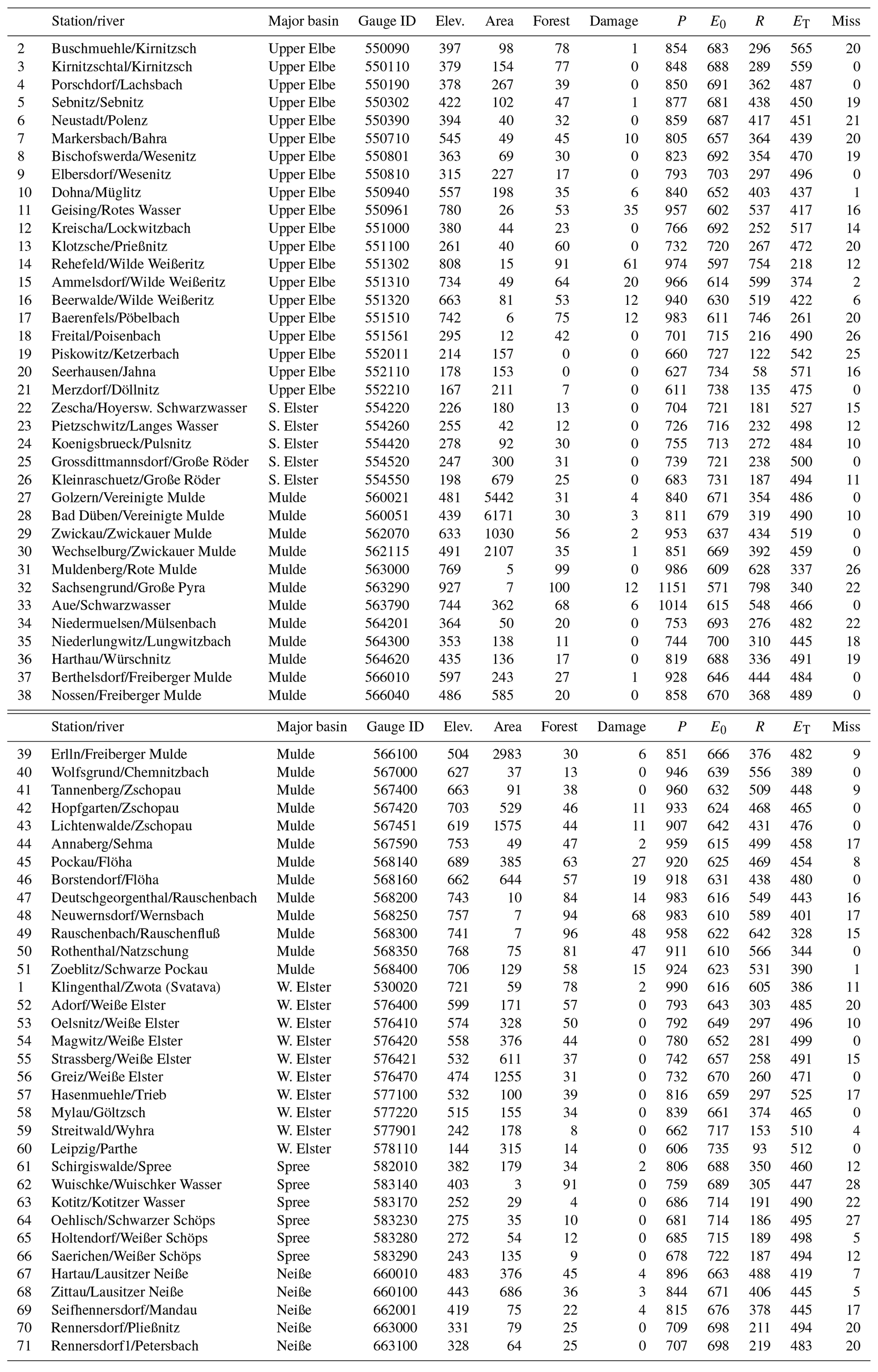
Table A1River stations analyzed over the period 1951–2020. The column “Elev.” denotes the mean catchment elevation in meters above sea level, “Area” denotes catchment area (in km2), and “Forest” gives the relative coverage of forest land use (%) based on CORINE 1990 data. Forest damage (in %) is given in the “Damage” column using the CORINE class 324. The columns P, E0, R, and ET denote average annual water balance components for the basins (in mm yr−1). The column “Miss” gives the number of missing years.
Groundwater aquifers in Saxony
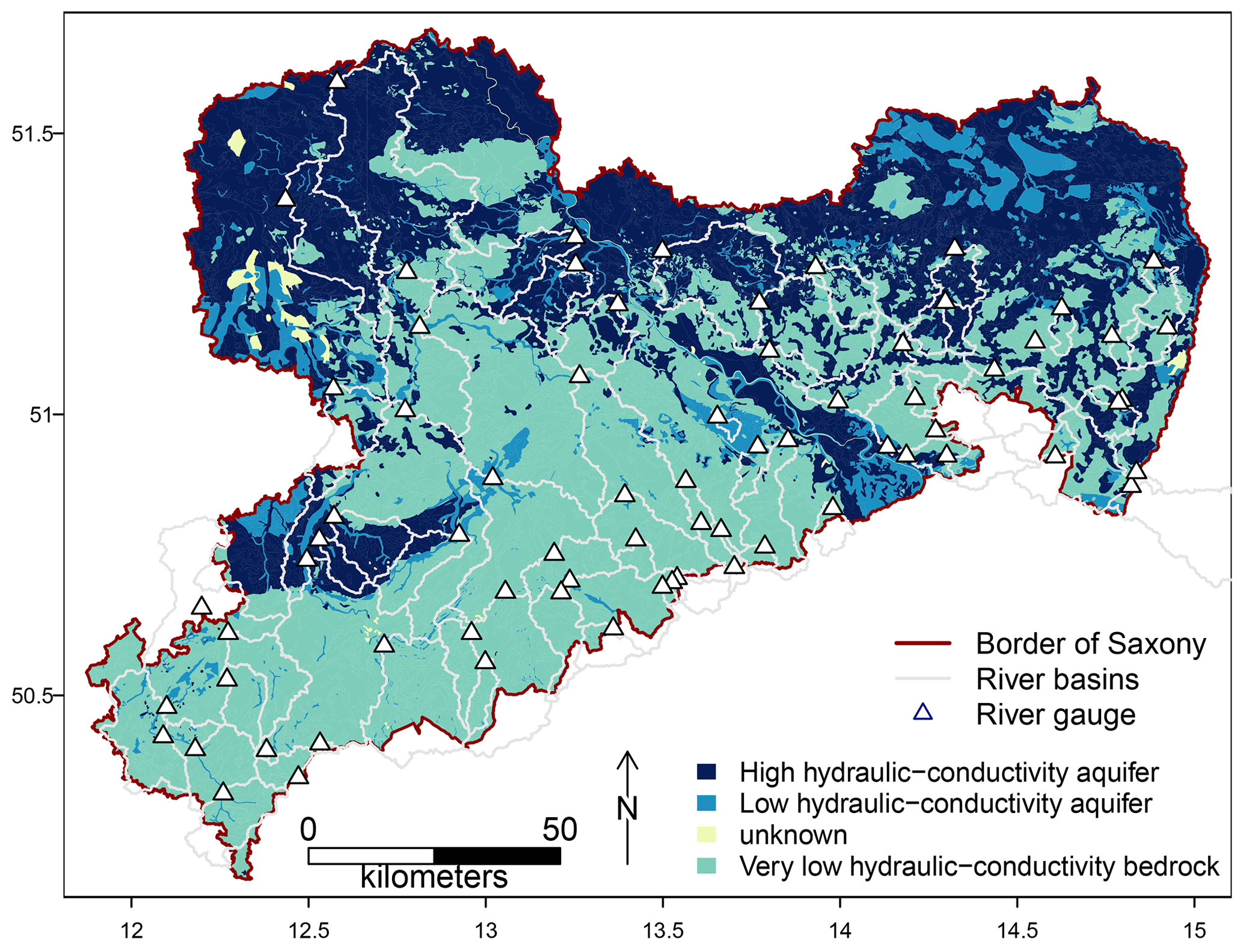
Figure A1Map of the Saxon hydrogeology categorized into highly conductive aquifers as strong indicators of large groundwater influences, lowly conductive aquifers for minor groundwater influence, and lowly conductive bedrock for regions without groundwater influences. Data source is the LfULG portal (https://www.umwelt.sachsen.de/umwelt/infosysteme/ida/index.xhtml, last access: 16 February 2024). On top, the river gauge locations and the catchment borders are plotted.
B1 Derivation of the decomposition for runoff
To get to Eq. (4), we start with the climate-induced change in evapotranspiration:
Next, we apply the water budget equation , which yields the climate part:
Then we can substitute ΔET,C to yield
You can rewrite and and insert both:
This yields Eq. (4):
To get to Eq. (5), we start with the land-cover-induced change in evapotranspiration, as noted in Sect. 2.2:
and we also apply the water balance equation to get to the runoff changes.
Then we can substitute ΔET,L to yield
By replacing ET,0 and ΔP, we get to the following equation:
We simplify this to achieve Eq. (5):
B2 Comparison of decomposition methods
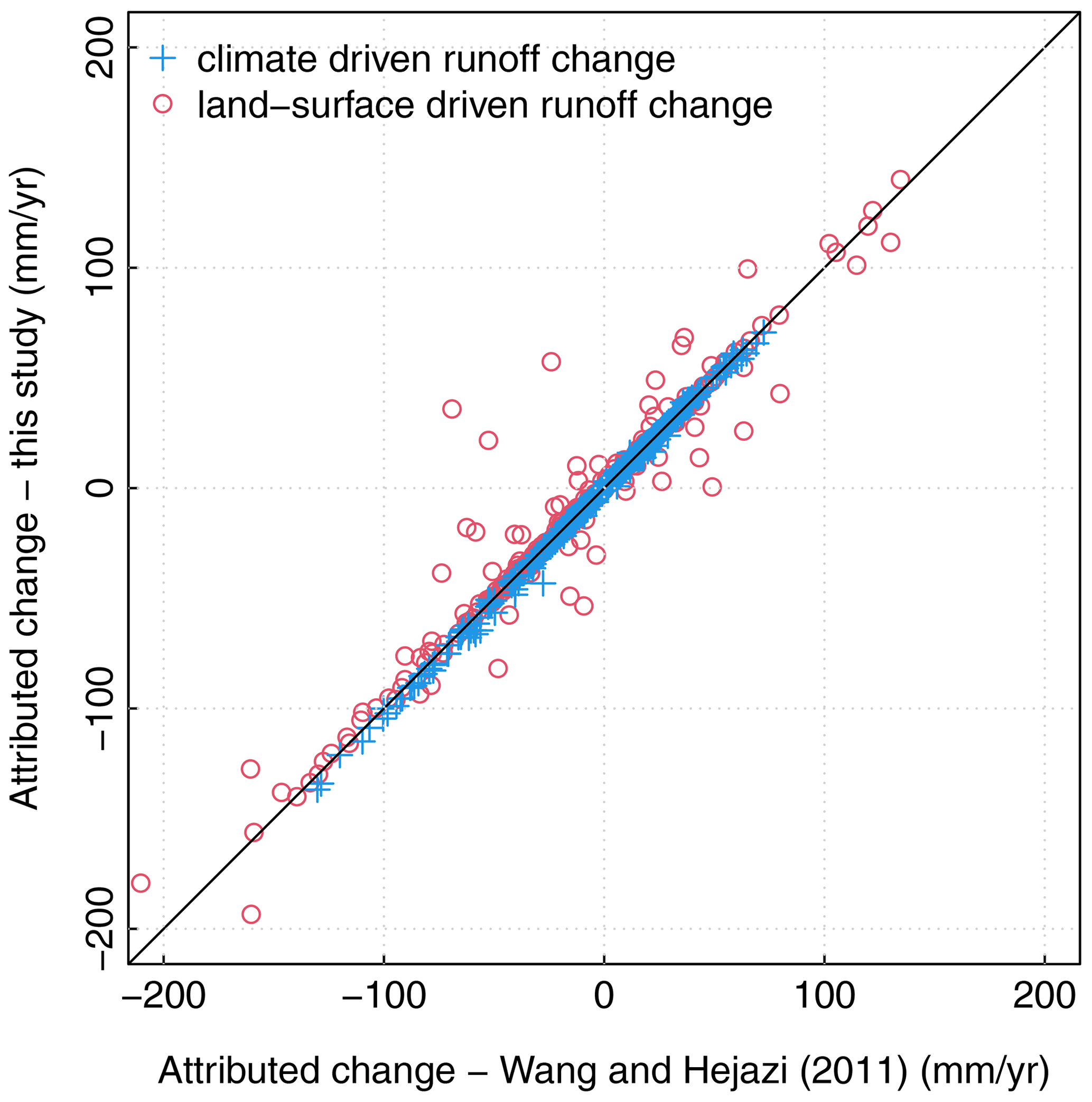
Figure B1Comparison of the decomposition method of this study with the method of Wang and Hejazi (2011) using the Mezentsev (1955) parametric Budyko function to separate climate- and land-surface-induced changes in runoff. Here, all decadal transitions of all catchments with sufficient data are used for the comparison.
Aggregated data and code to perform the analyses and to create the diagrams can be acquired from the first author.
MR conceived the study, acquired the data, and performed the analysis. MR and CH discussed the results and drafted the outline of the paper. CH provided information on the anthropogenic influences on catchment water budgets and hydrogeology. MR wrote the first draft of the paper, which was reviewed and edited by CH.
The contact author has declared that neither of the authors has any competing interests.
Publisher's note: Copernicus Publications remains neutral with regard to jurisdictional claims made in the text, published maps, institutional affiliations, or any other geographical representation in this paper. While Copernicus Publications makes every effort to include appropriate place names, the final responsibility lies with the authors.
We thank all the data providers for sharing their data. In particular, we thank the REKIS.org initiative, which collects meteorological data from different services for Saxony and bordering countries. Maik Renner is grateful to Rico Kronenberg (TU Dresden) for providing the daily data and Philipp Körner (IAMK GmbH, Dresden) for the discussion on reference evapotranspiration. For the hydrological data, we thank the Landesamt für Umwelt, Landwirtschaft und Geologie (LfULG) for providing most of their discharge data on the website, as well as Heike Mitzschke (Landeshochwasserzentrum, LfULG) for sending additional data and explanations on river gauge location data. Further, we thank Ralf Haupt (Hochwassernachrichtenzentrale, Thüringer Landesamt für Umwelt, Bergbau und Naturschutz) for providing the data of gauge Greiz/Weiße Elster. Finally, Maik Renner thanks Christian Bernhofer and Thomas Plunkte (TU Dresden) for the discussions on the ongoing changes related to the Wernersbach research catchment, which raised the motivation to extend the previous study from 2014.
This paper was edited by Elham R. Freund and reviewed by Tadd Bindas, Thiago Nascimento, and one anonymous referee.
Allen, R., Smith, M., Pereira, L., and Perrier, A.: An update for the calculation of reference evapotranspiration, ICID Bull., 43, 35–92, 1994. a, b, c, d
Arora, V.: The use of the aridity index to assess climate change effect on annual runoff, J. Hydrol., 265, 164–177, 2002. a
Berghuijs, W. R., Woods, R. A., and Hrachowitz, M.: A precipitation shift from snow towards rain leads to a decrease in streamflow, Nat. Clim. Change, 4, 583–586, https://doi.org/10.1038/nclimate2246, 2014. a, b
Bernhofer, C., Goldberg, V., Franke, J., Häntzschel, J., Harmansa, S., Pluntke, T., Geidel, K., Surke, M., Prasse, H., Freydank, E., Hänsel, S., Mellentin, U., and Küchler, W.: Klimamonographie für Sachsen (KLIMOSA) – Untersuchung und Visualisierung der Raum- und Zeitstruktur diagnostischer Zeitreihen der Klimaelemente unter besonderer Berücksichtigung der Witterungsextreme und der Wetterlagen, Sachsen im Klimawandel, Eine Analyse, Sächsisches Staats-Ministerium für Umwelt und Landwirtschaft, 211 pp., https://publikationen.sachsen.de/bdb/artikel/12173 (last access: 13 June 2024), 2008. a
Bosch, J. M. and Hewlett, J. D.: A review of catchment experiments to determine the effect of vegetation changes on water yield and evapotranspiration, J. Hydrol., 55, 3–23, https://doi.org/10.1016/0022-1694(82)90117-2, 1982. a
Bossard, M., Feranec, J., and Otahel, J.: CORINE land cover technical guide: Addendum 2000, European Environment Agency, Copenhagen, https://www.eea.europa.eu/publications/tech40add/download (last access: 13 June 2024), 2000. a
Budyko, M.: Evaporation under natural conditions, Gidrometeorizdat, Leningrad, English translation by IPST, Jerusalem, https://books.google.de/books/about/Evaporation_Under_Natural_Conditions.html?id=mS1RAAAAMAAJ (last access: 13 June 2024), 1948. a, b, c, d
Büntgen, U., Urban, O., Krusic, P. J., Rybníček, M., Kolář, T., Kyncl, T., Ač, A., Koňasová, E., Čáslavský, J., Esper, J., Wagner, S., Saurer, M., Tegel, W., Dobrovolný, P., Cherubini, P., Reinig, F., and Trnka, M.: Recent European drought extremes beyond Common Era background variability, Nat. Geosci., 14, 190–196, https://doi.org/10.1038/s41561-021-00698-0, 2021. a, b, c
Choudhury, B.: Evaluation of an empirical equation for annual evaporation using field observations and results from a biophysical model, J. Hydrol., 216, 99–110, 1999. a
Coxon, G., Freer, J., Westerberg, I. K., Wagener, T., Woods, R., and Smith, P. J.: A novel framework for discharge uncertainty quantification applied to 500 UK gauging stations, Water Resour. Res., 51, 5531–5546, https://doi.org/10.1002/2014WR016532, 2015. a
Dooge, J.: Sensitivity of runoff to climate change: A Hortonian approach, B. Am. Meteorol. Soc., 73, 2013–2024, 1992. a, b
Dyck, S. and Peschke, G.: Grundlagen der Hydrologie, Verlag für Bauwesen, Berlin, ISBN 978-3-345-00586-2, 1995. a
Fan, Y.: Are catchments leaky?, WIREs Water, 6, e1386, https://doi.org/10.1002/wat2.1386, 2019. a, b
Forstprojektierung: Aufnahme von Schadstufen bei Rauchschäden Betriebsregelungsanweisung – BRA IV/320, VEB Forstprojektierung, 1970. a
Franke, J. and Rühle, K.: Wetter trifft auf Klima, Jahresrückblick 2021, Tech. rep., Landesamt für Umwelt, Landwirtschaft und Geologie, Freistaat Sachsen, https://www.klima.sachsen.de/download/Jahresrueckblick2021_Fachbeitrag_final.pdf (last access: 13 June 2024), 2022. a, b, c
Fu, B.: On the calculation of the evaporation from land surface, Scient. Atmos. Sin., 5, 23–31, 1981. a
Gentine, P., D'Odorico, P., Lintner, B. R., Sivandran, G., and Salvucci, G.: Interdependence of climate, soil, and vegetation as constrained by the Budyko curve, Geophys. Res. Lett., 39, L19404, https://doi.org/10.1029/2012GL053492, 2012. a
Gudmundsson, L., Boulange, J., Do, H. X., Gosling, S. N., Grillakis, M. G., Koutroulis, A. G., Leonard, M., Liu, J., Müller Schmied, H., Papadimitriou, L., Pokhrel, Y., Seneviratne, S. I., Satoh, Y., Thiery, W., Westra, S., Zhang, X., and Zhao, F.: Globally observed trends in mean and extreme river flow attributed to climate change, Science, 371, 1159–1162, https://doi.org/10.1126/science.aba3996, 2021. a
Hannaford, J., Buys, G., Stahl, K., and Tallaksen, L. M.: The influence of decadal-scale variability on trends in long European streamflow records, Hydrol. Earth Syst. Sci., 17, 2717–2733, https://doi.org/10.5194/hess-17-2717-2013, 2013. a
Held, I. M. and Soden, B. J.: Robust responses of the hydrological cycle to global warming, J. Climate, 19, 5686–5699, https://doi.org/10.1175/JCLI3990.1, 2006. a
Hiemstra, P., Pebesma, E., Twenhöfel, C., and Heuvelink, G.: Real-time automatic interpolation of ambient gamma dose rates from the dutch radioactivity monitoring network, Comput. Geosci., 35, 1711–1721, 2009. a
Ionita, M., Nagavciuc, V., Kumar, R., and Rakovec, O.: On the curious case of the recent decade, mid-spring precipitation deficit in central Europe, npj Clim. Atmos. Sci., 3, 1–10, https://doi.org/10.1038/s41612-020-00153-8, 2020. a
Jaramillo, F. and Destouni, G.: Local flow regulation and irrigation raise global human water consumption and footprint, Science, 350, 1248–1251, https://doi.org/10.1126/science.aad1010, 2015. a
Jaramillo, F., Prieto, C., Lyon, S. W., and Destouni, G.: Multimethod assessment of evapotranspiration shifts due to non-irrigated agricultural development in Sweden, J. Hydrol., 484, 55–62, https://doi.org/10.1016/j.jhydrol.2013.01.010, 2013. a
Maas, R. and Grennfelt, P. (Eds.): Towards Cleaner Air. Scientific Assessment Report 2016, EMEP Steering Body and Working Group on Effects of the Convention on Long-Range Transboundary Air Pollution, Oslo, xx+50 pp., https://www.amap.no/documents/doc/towards-cleaner-air.-scientific-assessment-report-2016/1632 (last access: 14 June 2024), 2016. a, b, c, d
Masseroni, D., Camici, S., Cislaghi, A., Vacchiano, G., Massari, C., and Brocca, L.: The 63-year changes in annual streamflow volumes across Europe with a focus on the Mediterranean basin, Hydrol. Earth Syst. Sci., 25, 5589–5601, https://doi.org/10.5194/hess-25-5589-2021, 2021. a, b
Mazurski, K. R.: The destruction of forests in the polish Sudetes Mountains by industrial emissions, Forest Ecol. Manage., 17, 303–315, https://doi.org/10.1016/0378-1127(86)90158-1, 1986. a, b
Mezentsev, V.: More on the calculation of average total evaporation, Meteorol. Gidrol., 5, 24–26, 1955. a, b, c
Müller, U., Börke, P., and Mellentin, U.: Wie entwickeln sich die Wasserdargebote in Sachsen?, in: Wasserbau und Wasserwirtschaft im `Stresstest', Dresdner Wasserbauliche Mitteilungen 69, edited by: Technische Universität Dresden, Institut für Wasserbau und technische Hydromechanik, Dresden, 10–18, https://hdl.handle.net/20.500.11970/110912 (last access: 14 June 2024), 2023. a
Ol'Dekop, E.: On evaporation from the surface of river basins, Transactions on meteorological observations University of Tartu, 4, 200, 1911. a
Otto, L.-F., Matschulla, F., and Sonnemann, S.: Waldschutzsituation in Sachsen 2021, AFZ/Der Wald, https://www.sbs.sachsen.de/download/Waldschutzsituation_in_Sachsen_2021.pdf (last access: 14 June 2024), 2022. a, b
Pike, J.: The estimation of annual run-off from meteorological data in a tropical climate, J. Hydrol., 2, 116–123, 1964. a
Pitelka, L. F. and Raynal, D. J.: Forest Decline and Acidic Deposition, Ecology, 70, 2–10, https://doi.org/10.2307/1938405, 1989. a
Pluntke, T., Bernhofer, C., Grünwald, T., Renner, M., and Prasse, H.: Long-term climatological and ecohydrological analysis of a paired catchment – flux tower observatory near Dresden (Germany). Is there evidence of climate change in local evapotranspiration?, J. Hydrol., 617, 128873, https://doi.org/10.1016/j.jhydrol.2022.128873, 2023. a
Rakovec, O., Samaniego, L., Hari, V., Markonis, Y., Moravec, V., Thober, S., Hanel, M., and Kumar, R.: The 2018–2020 Multi-Year Drought Sets a New Benchmark in Europe, Earth's Future, 10, e2021EF002394, https://doi.org/10.1029/2021EF002394, 2022. a, b, c, d, e, f
Renner, M. and Bernhofer, C.: Long term variability of the annual hydrological regime and sensitivity to temperature phase shifts in Saxony/Germany, Hydrol. Earth Syst. Sci., 15, 1819–1833, https://doi.org/10.5194/hess-15-1819-2011, 2011. a, b, c
Renner, M., Seppelt, R., and Bernhofer, C.: Evaluation of water-energy balance frameworks to predict the sensitivity of streamflow to climate change, Hydrol. Earth Syst. Sci., 16, 1419–1433, https://doi.org/10.5194/hess-16-1419-2012, 2012. a
Renner, M., Brust, K., Schwärzel, K., Volk, M., and Bernhofer, C.: Separating the effects of changes in land cover and climate: a hydro-meteorological analysis of the past 60 yr in Saxony, Germany, Hydrol. Earth Syst. Sci., 18, 389–405, https://doi.org/10.5194/hess-18-389-2014, 2014. a, b, c, d, e, f, g, h, i, j, k, l, m, n, o, p, q, r, s
Schreiber, P.: Über die Beziehungen zwischen dem Niederschlag und der Wasserführung der Flüsse in Mitteleuropa, Z. Meteorol., 21, 441–452, 1904. a, b
SMUL: Waldzustandsbericht 2006 Freistaat Sachsen, in: Waldzustandsbericht, Sachsenforst, Pirna, https://publikationen.sachsen.de/bdb/artikel/10758 (last access: 14 June 2024), 2006. a, b
Šrámek, V., Slodičák, M., Lomskỳ, B., Balcar, V., Kulhavỳ, J., Hadaš, P., Pulkráb, K., Šišák, L., Pěnička, L., and Sloup, M.: The Ore Mountains: Will successive recovery of forests from lethal disease be successful, Mount. Res. Dev., 28, 216–221, 2008. a, b
Statistisches Landesamt Freistaat Sachsen: Bodennutzung und Ernte im Freistaat Sachsen, Statistischer Bericht C II 2 - j/21, https://www.statistik.sachsen.de/download/statistische-berichte/statistik_sachsen_cII2_bodennutzung-ernte.xlsx (last access: 14 June 2024), 2022. a
Teuling, A. J., Seneviratne, S. I., Stöckli, R., Reichstein, M., Moors, E., Ciais, P., Luyssaert, S., van den Hurk, B., Ammann, C., Bernhofer, C., Dellwik, E., Gianelle, D., Gielen, B., Grünwald, T., Klumpp, K., Montagnani, L., Moureaux, C., Sottocornola, M., and Wohlfahrt, G.: Contrasting response of European forest and grassland energy exchange to heatwaves, Nat. Geosci., 3, 722–727, https://doi.org/10.1038/ngeo950, 2010. a
Teuling, A. J., de Badts, E. A. G., Jansen, F. A., Fuchs, R., Buitink, J., Hoek van Dijke, A. J., and Sterling, S. M.: Climate change, reforestation/afforestation, and urbanization impacts on evapotranspiration and streamflow in Europe, Hydrol. Earth Syst. Sci., 23, 3631–3652, https://doi.org/10.5194/hess-23-3631-2019, 2019. a
Todorov, V. and Filzmoser, P.: An Object-Oriented Framework for Robust Multivariate Analysis, J. Stat. Softw., 32, 1–47, https://doi.org/10.18637/jss.v032.i03, 2009. a
Turc, L.: Evaluation des besoins en eau d'irrigation, évapotranspiration potentielle, Ann. Agron., 12, 13–49, 1961. a
Wang, D. and Hejazi, M.: Quantifying the relative contribution of the climate and direct human impacts on mean annual streamflow in the contiguous United States, Water Resour. Res., 47, W00J12, https://doi.org/10.1029/2010WR010283, 2011. a, b, c, d, e
Wild, M., Gilgen, H., Roesch, A., Ohmura, A., Long, C. N., Dutton, E. G., Forgan, B., Kallis, A., Russak, V., and Tsvetkov, A.: From Dimming to Brightening: Decadal Changes in Solar Radiation at Earth's Surface, Science, 308, 847–850, https://doi.org/10.1126/science.1103215, 2005. a
Zhang, L., Dawes, W., and Walker, G.: Response of mean annual evapotranspiration to vegetation changes at catchment scale, Water Resour. Res., 37, 701–708, 2001. a