the Creative Commons Attribution 4.0 License.
the Creative Commons Attribution 4.0 License.
 | 28 Jun 2024
Technical note: Removing dynamic sea-level influences from groundwater-level measurements
Patrick Haehnel
Todd C. Rasmussen
Gabriel C. Rau
The sustainability of limited freshwater resources in coastal settings requires an understanding of the processes that affect them. This is especially relevant for freshwater lenses of oceanic islands. Yet, these processes are often obscured by dynamic oceanic water levels that change over a range of timescales. We use regression deconvolution to estimate an oceanic response function (ORF) that accounts for how sea-level fluctuations affect measured groundwater levels, thus providing a clearer understanding of recharge and withdrawal processes. The method is demonstrated using sea-level and groundwater-level measurements on the island of Norderney in the North Sea (northwestern Germany). We expect that the method is suitable for any coastal groundwater system where it is important to understand processes that affect freshwater lenses or other coastal freshwater resources.
- Article
(6642 KB) - Full-text XML
-
Supplement
(10275 KB) - BibTeX
- EndNote


Groundwater is often the dominant source of freshwater on oceanic islands, and the sustainable management of this resource relies on understanding the gains (recharge) and losses (discharge, withdrawals) that are a function of the dynamic forces that act upon it (White and Falkland, 2009). Because freshwater on oceanic islands typically occurs as a lens above denser, saline seawater (Underwood et al., 1992), groundwater withdrawals alter fluid pressures and affect the interface between freshwater and saltwater. Excessive groundwater extraction can lead to aquifer salinization due to horizontal seawater intrusion, as well as vertical upconing (Barlow, 2003; Falkland, 1991). Thus, island groundwater resources are among the most vulnerable in the world, stressing the need for careful monitoring and understanding to sustain their productivity (White and Falkland, 2009).
Estimating groundwater recharge on oceanic islands is challenging because groundwater levels in such systems are highly dynamic and can be influenced by multiple factors, such as periodic and aperiodic sea-level changes, coastal morphology, aquifer properties, precipitation, and withdrawals (Jiao and Post, 2019), that interact to influence near-shore groundwater levels (e.g., Patton et al., 2021). Several methods have been used for estimating groundwater recharge, such as lysimeters (e.g., Stuyfzand, 2017), tritium–helium age dating (e.g., Houben et al., 2014; Röper et al., 2012), and stable-isotope methods (e.g., 18O, 2H, see Koeniger et al., 2016; Post et al., 2022). However, temporal differentiation of the recharge, which is critical for understanding the dynamics of coastal groundwater systems, is costly and time intensive using these methods.
Regression deconvolution provides an alternative method for quantifying groundwater processes using real-time, groundwater-level measurements. The method has been successfully applied to remove the influence of barometric pressure (Furbish, 1991; Rasmussen and Crawford, 1997), Earth tides (Toll and Rasmussen, 2007), near-surface water content (Rasmussen and Mote, 2007), and river stages (Spane and Mackley, 2011) from groundwater-level time series. Yet, despite its versatility, applications using convolution methods are commonly missing from hydrogeology textbooks (Olsthoorn, 2008). Convolution by means of transfer function noise modeling has been applied by Bakker and Schaars (2019) to model hydraulic heads of a coastal aquifer based on time series from sea level, recharge, and groundwater withdrawal. An estimation of a response function from sea-level data itself and from the removal of sea-level influences from dynamic groundwater levels in coastal settings, as has been done with regression deconvolution, has not been performed (to the authors' knowledge). Especially in coastal settings, periodic and aperiodic influences often obscure important groundwater processes, such as recharge – which is difficult to estimate or directly measure – and pumping.
The objective of this work is to (i) provide a generic formulation for regression deconvolution, (ii) demonstrate the use of regression deconvolution for removing sea-level influences from groundwater-level measurements in an unconfined coastal aquifer consisting of unconsolidated sediments, and (iii) illustrate how the method is useful for coastal groundwater systems. The application uses groundwater-level, sea-level, and meteorologic data collected on the coastal island of Norderney, located in northwestern Germany in the North Sea. We believe that our method is suitable for application in other coastal aquifers to support their sustainable management by better understanding the processes within – and physical characteristics of – freshwater lenses.
2.1 Conceptual overview
Figure 1 presents our conceptual model of the influence of sea levels on groundwater in coastal islands. Note that a freshwater lens is present above an underlying saltwater zone, where the depth to the freshwater–saltwater interface is a function of the water table elevation above mean sea level, as defined by the Ghyben–Herzberg principle (Jiao and Post, 2019; Post et al., 2018).
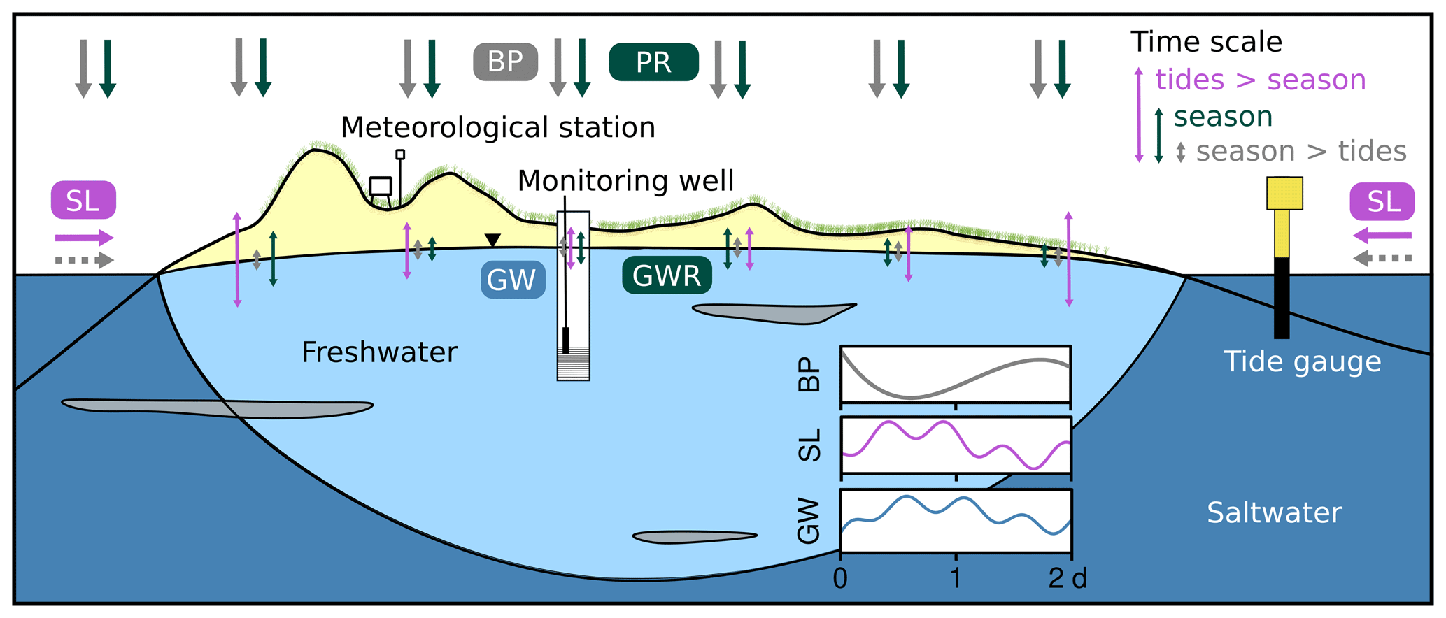
Figure 1Conceptual model of groundwater-level fluctuations (GW) on a coastal island with barometric-pressure (BP), sea-level (SL), and groundwater-recharge (GWR) forcing. The latter results from precipitation (PR) on oceanic islands. Note that the amplitude of groundwater fluctuations is larger for tidal influences near the shoreline than for seasonal influences but smaller toward the center of the island. The left-hand side of the island constitutes the seaward side, while the right-hand side constitutes the leeward side of the island. Seasonal influences diminish on the leeward side of the island. Dotted gray lines indicate the indirect influence of barometric pressure through sea levels on the groundwater levels.
Barometric influences within unconfined aquifers are a function of the depth of the water table below the ground surface and the air diffusivity within the unsaturated zone (Rasmussen and Crawford, 1997). Barometric pressure displays diurnal fluctuations due to solar heating, along with seasonal and weather-related forcing (McMillan et al., 2019).
Sea-level variation is dominated by diurnal and semi-diurnal periodicities, along with aperiodic behavior resulting from storm events (Boon, 2011). Further, waves breaking at the shore impact groundwater-level dynamics (e.g., Nielsen, 1999; Housego et al., 2021). Wave dynamics generally occur at high frequencies at the shoreline (e.g., Stockdon et al., 2006; Hegge and Masselink, 1991), while the continuous wave breaking at the shore results in a more persistent, lower-frequency wave setup (Stockdon et al., 2006; Gomes da Silva et al., 2020). Wave setup is generally larger during storm events (e.g., Senechal et al., 2011) and thus adds to the magnitude of the storm-event-related, aperiodic rises in sea level.
The influence of fluctuating sea levels and waves diminishes with distance from the shoreline, with tidal and high-frequency wave variations attenuating more rapidly than variations with the seasons; wave setup; or extreme events, such as floods or droughts (Ferris, 1952; Li et al., 2004; Nielsen, 1990; Li et al., 1997; Cartwright et al., 2006; Rotzoll and El-Kadi, 2008). Precipitation recharges groundwater by vertical percolation through the overlying unsaturated zone or by direct recharge from surface waterbodies that fill during storm events.
Note that changes in barometric pressure also affect sea level (Boon, 2011) so that the barometric influence is introduced into groundwater-level time series of coastal aquifers in two principal directions: (i) vertically, through the direct influence of changes in barometric pressure, and (ii) horizontally, through the indirect influence of barometric pressure on the sea level, which is carried through the aquifer with the propagating sea-level signal (Fig. 1). Hence, the barometric influence affects groundwater levels at different time lags through the vertical and horizontal components.
2.2 Single-factor regression deconvolution
Barometric-pressure changes often influence groundwater levels in both confined and unconfined aquifers. The barometric efficiency (BE) is commonly used to describe the instantaneous linear relationship between discrete changes in barometric-pressure ΔBP and groundwater-level responses ΔGW (Rasmussen and Crawford, 1997):
While groundwater responses to barometric-pressure changes are frequently assumed to be instantaneous, there is often a delayed response that depends upon the degree of confinement, the depth to water table, borehole-storage effects, whether the borehole is open or sealed, and whether an absolute or relative (gauge) pressure sensor is used (Rojstaczer and Riley, 1990; Rasmussen and Crawford, 1997).
Response functions β(τ) are commonly used to quantify the time-lagged response caused by an impulse input x(t) to the output time series y(t) using the convolution operator ⋆:
where K is the maximum number of time lags; t is the observation time; and τk=kΔt is the time lag between the input and the observed response, with the sampling interval Δt (Rasmussen and Mote, 2007; Rau et al., 2020). We define m=τK, which is the maximum time lag or memory of the system, beyond which the output is unaffected by an input (Rasmussen and Mote, 2007). Convolution assumes a linear, time-invariant system, with responses to individual inputs being independent of other inputs.
While convolution is used to find the output function y(t) as a function of the response function β(τ) and the input function x(t), we are often interested in finding the response function by inversion of the input and output time series using the deconvolution operator \ (i.e., backslash):
Deconvolution can be implemented using multiple regression by forming a set of linear equations:
where the left-hand side shows the observed outputs, and the right-hand side consists of the unknown response function values and lagged input values (Toll and Rasmussen, 2007). This equation is written in matrix form as
where y is the [1×n] row vector of n observed outputs; β is the [1×m] row vector of unknown response coefficients; and X is the [m×n] matrix of observed inputs, with each row being lagged by 1 time unit. Note that the first m columns of y and X must be omitted unless prior input data are available; i.e., observations may be lacking for x(t−m).
The resulting matrix equation can be solved using ordinary least-squares (OLS) regression, which takes the matrix form
where the superscripts [⋅]T and indicate the matrix transpose and inverse, respectively, and where alternative matrix solvers are likely to be more efficient and accurate. The reconstructed (fitted) time series, , can then be used to find the residual, as well as a time series that is corrected from the process influence as follows:
The term “corrected” is used in this work and in the literature in relation to regression deconvolution to mean that “the influence of a process on the time series was removed”. The use of the term corrected does not suggest any kind of error in the original time series.
The deconvolution was performed using first differences of the measurements, leading to Eq. (5) becoming
This removes the effect of persistent trends in the data and therefore avoids a bias in the regression (Rasmussen and Crawford, 1997; Butler et al., 2011). To avoid spurious influences from the fact that the reconstruction hinges on an initial groundwater measurement that cannot be corrected, the mean of the corrected time series was matched to the uncorrected one.
2.3 Multi-factor regression deconvolution
Toll and Rasmussen (2007) and Butler et al. (2011) presented a method to analyze and remove both barometric pressure and Earth tides (i.e., two independent processes) from groundwater levels. This procedure can be extended to account for multiple drivers as follows:
Here, ΔXp is the time series of the differences in the influencing process p, P represents the total number of processes, βp(τk) represents the time-lagged impulse response function coefficients for process p, and is the total memory for process p. Note that all processes propagate through the subsurface either vertically or horizontally and are increasingly attenuated and time-lagged with distance from their origin. This approach allows us to consider multiple dynamic processes that could affect groundwater levels, including precipitation, evapotranspiration, barometric pressure, streamflow, Earth tides, soil moisture, etc. Note that process-based indices are always notated as superscripts here.
2.4 Process response functions and time series correction
The response function for a process is determined from the impulse responses (Eq. 6) as follows:
Note that we state the process response function Bp as a generic term that allows disentanglement of multiple processes p, each with total memory mp. For example, the barometric response function (BRF) is determined by taking the cumulative sum of the impulse responses to barometric pressure (Rasmussen and Crawford, 1997):
Analogously, an Earth tide response function (ETRF), as well as a river response function (RRF), can be formulated in the same way. These influences have successfully been used to characterize subsurface processes and properties and to correct groundwater levels for the respective aforementioned influences (e.g., Spane, 2002; Toll and Rasmussen, 2007; Butler et al., 2011; Spane and Mackley, 2011; Rau et al., 2020). Here, we note that, despite being used to correct groundwater levels, the name ETRF has not explicitly been defined in the literature.
The aim of this work is to illustrate how regression deconvolution can be used to estimate the oceanic response function (ORF):
This characterizes the effects of sea-level fluctuations SL(t) on measured groundwater levels:
with sea-level memory mSL. We note that our approach employs multi-factor regression deconvolution to disentangle the simultaneous influences of sea levels and barometric pressure on observed groundwater levels; thus, processes in Eq. (9). We did not analyze Earth tide responses as they are generally negligible in unconfined finite-depth aquifers made of unconsolidated sediment (Rojstaczer and Riley, 1990). The formulated correction procedure yields corrected groundwater levels:
Again, the mean of the corrected values must be matched to the mean of the uncorrected values (as explained earlier).
A wave response function and groundwater levels with wave setup removed can be obtained equivalently, e.g., to account for additional storm-event-related wave setup at the shore. Alternatively, wave setup can be incorporated into the sea-level time series to obtain an ORF representing both processes. Note that wave setup is generally estimated from offshore wave measures (e.g., Gomes da Silva et al., 2020).
Besides regression deconvolution, transfer function noise models are used to model groundwater-level time series from time series of stresses (e.g., groundwater recharge, groundwater extraction, sea levels) using convolution (e.g., von Asmuth et al., 2002; Collenteur et al., 2019; Bakker and Schaars, 2019) and to estimate unknown stresses from groundwater-level time series (e.g., Collenteur et al., 2021; Pezij et al., 2020). The method differs from regression deconvolution in that the response function is pre-defined with a fixed shape, typically by a probability density function like the Gamma distribution (Collenteur et al., 2019), and is not obtained through the data itself.
2.5 Considering density effects
The density difference between seawater and freshwater has to be considered when applying Eqs. (8), (9), and (14) with sea levels present in ΔX. Here, the ORF is defined based on hydraulic-head measurements in freshwater. The propagation of external influences in the aquifer depends on the pressure of the external stressor rather than the elevations, which are used as a proxy (i.e., hydraulic heads). A change of hydraulic head in seawater yields a larger pressure change than the same hydraulic head change in freshwater would due to the density difference. Therefore, sea-level records need to be corrected for this higher density to correctly represent the pressure changes in sea level at the shore with reference to fresh groundwater inland.
Density correction of hydraulic heads is typically achieved by calculating freshwater heads:
where h is the measured point water head, ρf is the freshwater density (1000 kg m−3), and ρ is the density of the water at the screen elevation z of a monitoring well (Post et al., 2007). In the case of sea-level observations, ρ is the seawater density, and z is the elevation of the sea floor. When using first differences, the freshwater head difference between times ti and ti−1 is
whereby sea-level differences in Eqs. (9) and (14) have to be defined as freshwater-equivalent differences:
This corrects differences in measured sea levels ΔXSL by the density ratio between saltwater and freshwater.
Should the groundwater monitoring well be screened in a location of brackish water or saltwater, the density correction needs to be applied to the hydraulic-head differences as well to obtain freshwater-equivalent hydraulic-head differences:
This way, ORFs which are comparable between monitoring sites can be obtained. Especially at beach sites, the density ratio may be a function of time reflective of salinity changes over time around the screen of the monitoring well (Grünenbaum et al., 2023; Greskowiak and Massmann, 2021). Details on the estimation of groundwater density from electric conductivity measurements are provided by Post (2012).
3.1 Field site, monitoring, and data processing
Norderney is a coastal barrier island that is part of the East Frisian island chain located in the North Sea near the northwestern German coast (Fig. 2). The island covers an area of about 25 km2, with an east-to-west extent of 14 km and an average north-to-south extent of 2 km (Naumann, 2005; Streif, 1990). Rainfall is the only source of freshwater on the island, and 782 mm of precipitation was observed during our 1-year research period (1 November 2018 to 31 October 2019) at the Norderney meteorological station (DWD Climate Data Center, 2021a). Approximately half of the island's precipitation was estimated to recharge the aquifer (Naumann, 2005).
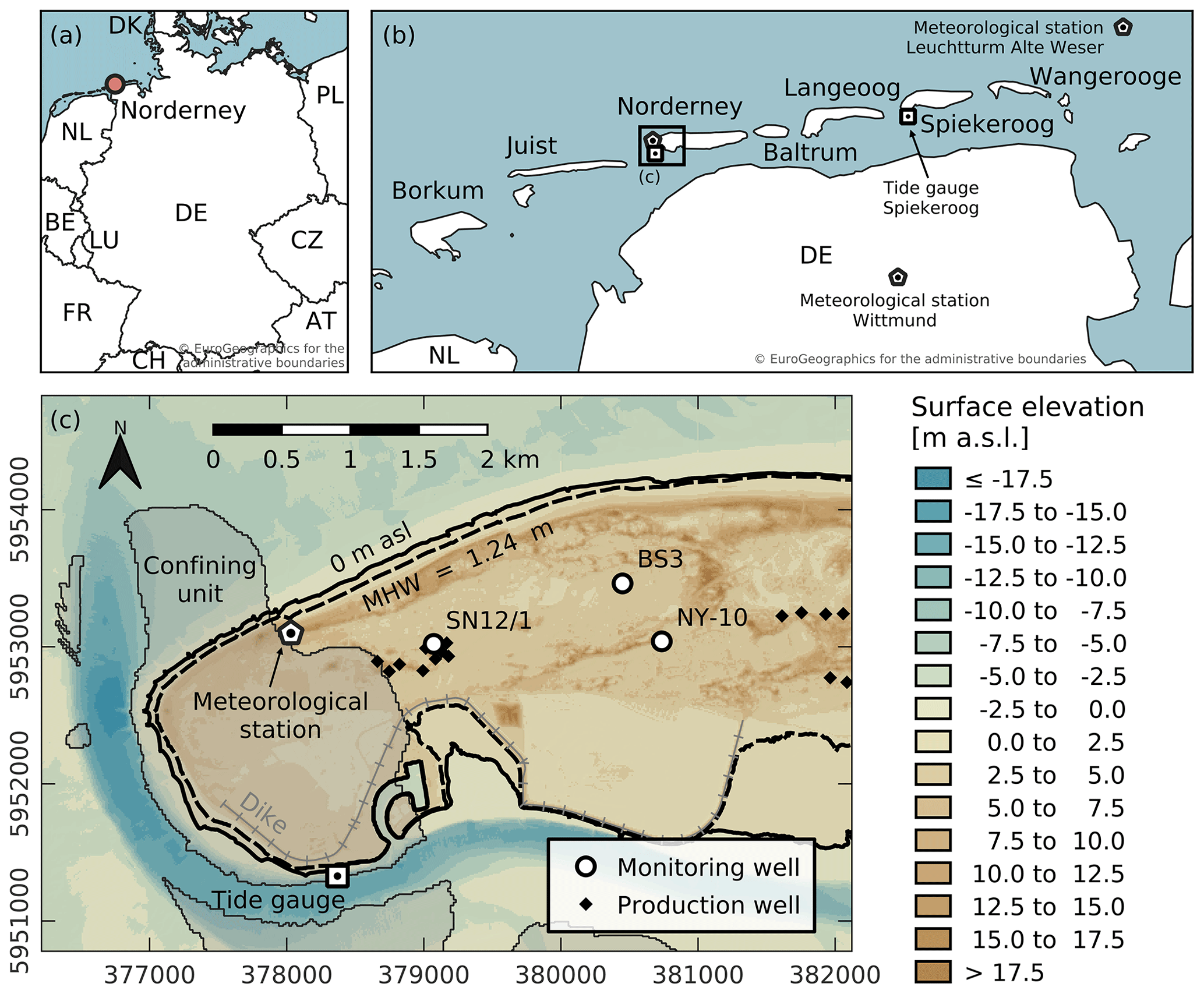
Figure 2Map of the island of Norderney in northwestern Germany showing three monitoring wells, production wells, the tide gauge, the meteorological station, and a confining unit (shaded area) to the west. Mean high water (MHW) is the average between 2010 and 2020 (WSA Ems-Nordsee, 2021). Coordinate reference system is UTM Zone 32N (EPSG:25832). Data sources: EuroGeographics and UN-FAO (2020); © EuroGeographics for the administrative boundaries; Haehnel et al. (2023); NLWKN (2021); Sievers et al. (2020); Stadtwerke Norderney (2021b); WSA Ems-Nordsee (2021).
Semi-diurnal tides dominate Norderney's sea-level fluctuations. For our research period, the mean high water (MHW) was 1.26 m a.s.l. (above sea level), and the mean low water (MLW) was −1.18 m a.s.l. (WSA Ems-Nordsee, 2021), which yields a tidal range of 2.44 m that corresponds to meso-tidal conditions (Hayes, 1979). Seasonal flooding typically occurs during the autumn and winter seasons (Holt et al., 2019) and is defined using a sea level 1.5 m above the MHW for the region (Gönnert, 2003). The maximum sea level during our study period was 3.03 m a.s.l. (1.77 m above MHW) on 8 January 2019 (WSA Ems-Nordsee, WSA Ems-Nordsee, 2021).
The island's geomorphology is characterized by beaches and dunes on the seaward north and salt marshes and back-barrier tidal flats on the leeward south (Petersen et al., 2003). Holocene dune sediments are composed of fine-grained sands and sand flat with mixed flat deposits, extending to about 30 to 40 m b.s.l. (below sea level) in the central part of the island (Naumann, 2005; Streif, 1990). These sediments extend to a depth of about 10 m b.s.l. below the western part of the island, where they transition to a confining unit of Holocene clay, silt, and basal peat (Schaumann et al., 2021), shown in Fig. 2c. Mud flat deposits are present locally below the central part of the island (Naumann, 2005). Pleistocene sandy deposits are found below Holocene sediments, which largely originated from Drenthian sandur-type plains (Naumann, 2005; Schaumann et al., 2021).
A more detailed summary of the island's development, geomorphology, geology, and hydrogeology can be found in Haehnel et al. (2023). Schaumann et al. (2021) described the Holocene and Pleistocene geology in detail, and Karle et al. (2021) reconstructed the Holocene landscape development of the area during sea-level transgression.
Hourly groundwater levels are routinely collected by the Municipal Works Norderney using STS DL/N 70 data loggers in open (uncapped) monitoring wells (Stadtwerke Norderney, 2021a). This study focuses on a subset of these wells (SN12/1, BS3, NY-10) for the 1-year period between 1 November 2018 and 31 October 2019. At the given time series length of 1 year, time increments of 1 h are generally sufficient to capture the tidal constituents present at the study site (Schweizer et al., 2021). As summarized in Table 1, the monitoring wells have short (1 to 2 m) screen lengths. Both the BS3 and NY-10 screened zones are shallow, while SN12/1 has a deeper screen from 18 to 20 m b.s.l., which is below the base elevation of the nearby confining unit (Fig. 2c; Haehnel et al., 2023). All three observation wells are screened entirely in the freshwater lens of the island. Both SN12/1 and BS3 are located at similar straight-line distances (688 and 741 m, respectively) from the shoreline (i.e., the 0 m a.s.l. contour line), while NY-10 is located more centrally on the island at a greater distance (1154 m) (Table 1). The distance to the MHW contour line is also presented in Table 1 because the shoreline distance is ambiguous when tides are present.
Table 1Reference data for the groundwater monitoring wells (Stadtwerke Norderney, 2021b). Coordinate reference system is UTM Zone 32N (EPSG:25832).
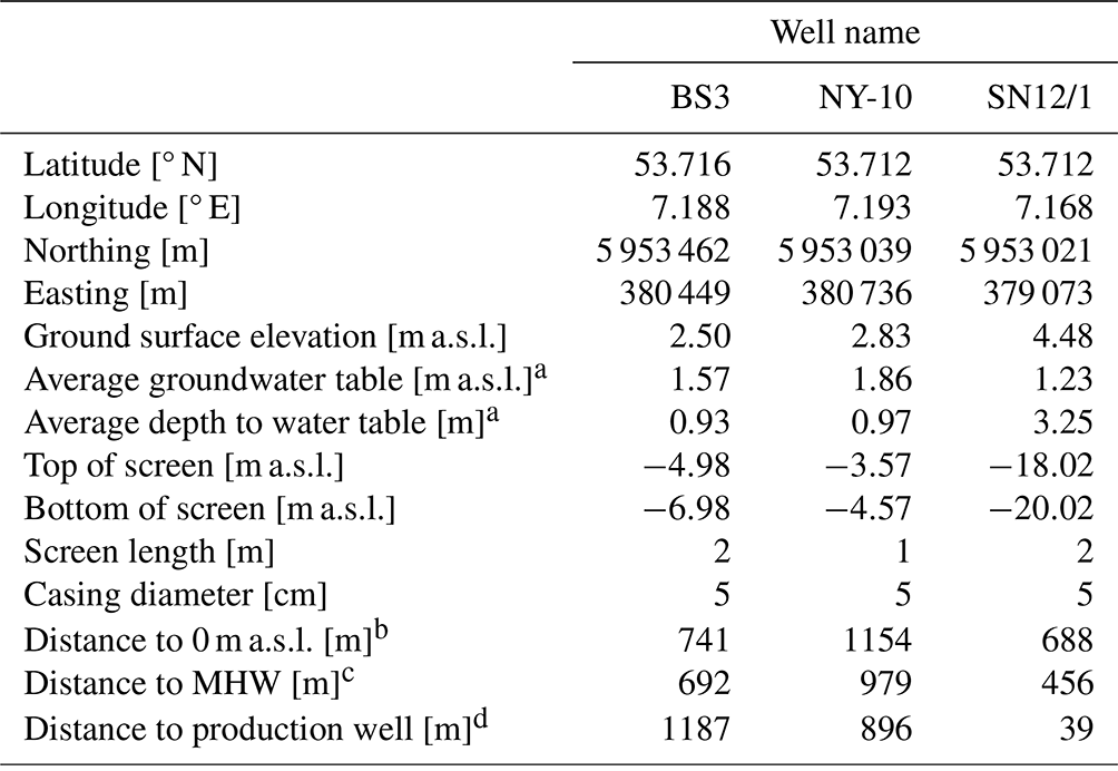
a Averaged over the studied time frame from 1 November 2018 to 31 October 2019. b Minimum Euclidean distance to 0 m a.s.l. contour using a DEM of Sievers et al. (2020). c Minimum Euclidean distance to mean high water (MHW) contour (1.24 m a.s.l., average between 2010 and 2020 from WSA Ems-Nordsee, 2021) using a DEM of Sievers et al. (2020). d Euclidean distance to closest production well.
Hourly barometric-pressure and precipitation data were obtained from the meteorological station located near the northwestern shoreline (DWD Climate Data Center, 2021b, c). The spatial distance between the meteorological station and the groundwater monitoring wells is approximately 1 km in the case of SN12/1 and approximately 2.5 km in the case of BS3 and NY-10. At this distance, the barometric-pressure observations are assumed to be representative for the groundwater monitoring locations as the barometric pressure typically varies at larger spatial scales (see Appendix A). Daily precipitation totals are used for graphical comparison with other variables (DWD Climate Data Center, 2021a).
Sea levels collected at 1 min intervals were obtained from the tide gauge Norderney Riffgat (WSV, 2021a), located near the southwestern shoreline. Tidal data were downsampled to hourly intervals for subsequent analysis by discarding observation time points that did not match the sampling times of groundwater and barometric-pressure data, which were collected at each full hour. Sea-level differences as required for Eq. (14) were converted to freshwater-equivalent sea-level differences according to Eq. (17), with the density ratio , assuming a saltwater density of 1025 kg m−3 at the study site. The spatial distance of the tide gauge from the shoreline segments closest to the observation wells should not affect the results presented here because the temporal offset of the sea-level signal at these shoreline segments compared to the tide gauge is on the order of a few minutes, much shorter than the sampling interval of 1 h used in this study (see Appendix A). An hourly time series of the extracted water volume from the western production well cluster near SN12/1 (Fig. 2c) between 13 and 20 November 2022 was provided by the local water supplier (Stadtwerke Norderney, 2023).
Groundwater and tidal data were inspected prior to analysis, and no issues (e.g., gaps, spikes, steps) were found. Barometric-pressure and precipitation data were examined by the data provider using an automated evaluation and correction procedure (DWD Climate Data Center, 2021a, c, b). No data were missing in any time series related to Norderney during the research period. All data were converted to the time zone UTC+1.
The low-pass finite-impulse-response filter LP241H079122kM3 from Shirahata et al. (2016) was applied to groundwater and sea levels for comparison with regression deconvolution results. The filter uses a 10 d symmetric window designed to remove diurnal and semi-diurnal tidal constituents, as well as their higher harmonics.
3.2 Processes affecting groundwater levels
Sea-level, barometric-pressure, and daily precipitation data are presented in Fig. 3a and b. Note the aperiodic meteorological influences, as well as the sea-level influences, which are dominated by astronomical tides, on groundwater levels (Fig. 3c–e). This demonstrates the overlapping effects of both the vertical propagation of atmospheric effects and the lateral effects of sea-level variation. Groundwater levels show an oscillating semi-diurnal pattern with differing magnitudes due to sea-level influences that propagate through the aquifer (Fig. 3c–e) and reflect both periodic and aperiodic changes in sea level (e.g., the storm event on 8 January 2019). The well furthest from the shoreline, NY-10, shows the strongest attenuation of the oscillating sea levels, while the attenuation in BS3 and SN12/1 is smaller due to the wells' greater proximity to the shoreline. Yet, BS3 is more strongly attenuated than SN12/1 despite their similar distances from the shoreline. This is likely explained by the nearby confining unit in the west (Fig. 2) that allows the signal to propagate more rapidly due to a smaller storativity.
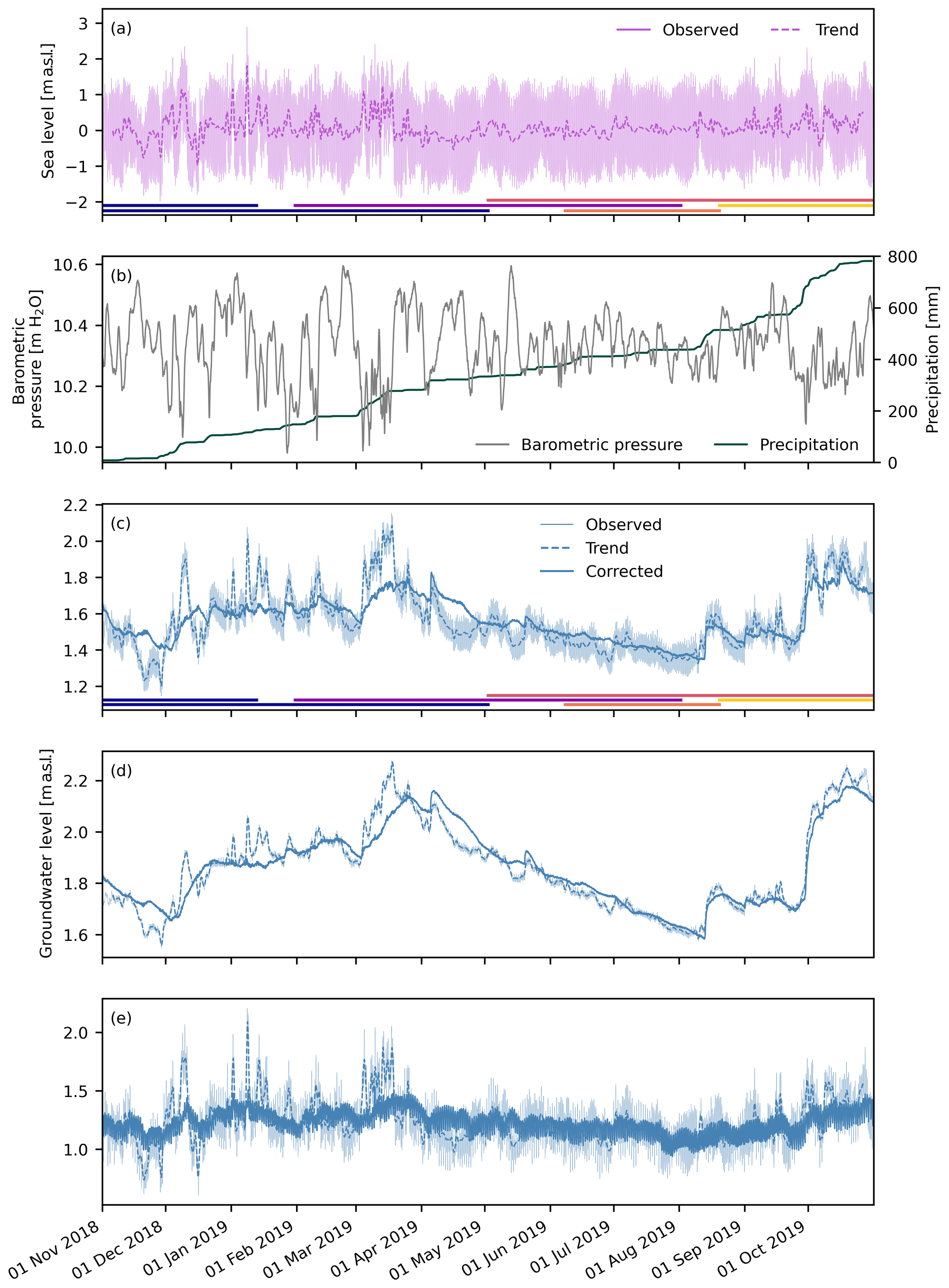
Figure 3Time series of (a) sea level; (b) barometric pressure and cumulative daily precipitation; and observed and corrected groundwater levels in (c) BS3, (d) NY-10, and (e) SN12/1. Oceanic response function memories mSL are 150, 250, and 48 h, respectively, while the barometric response function memory mBP is 24 h for each monitoring well. Trends in sea and groundwater levels are also shown in (a) and (c)–(e). Horizontal colored bars in (a) and (c) indicate the time frames covered by shorter portions of the time series for which the ORF was calculated (Fig. 5).
In addition to changes in sea level, groundwater levels in BS3 and NY-10 show precipitation responses, but these are largely obscured in SN12/1. The precipitation response of BS3 and NY-10 is discernible in mid-August 2019, where groundwater levels increase despite a lack of change in sea levels. Also note that groundwater levels increase, while sea levels decrease in late September to early October 2019.
3.3 Removing dynamic sea-level influences
Periodic and aperiodic sea-level fluctuations as well as barometric-pressure fluctuations were removed from groundwater-level measurements using regression deconvolution (Fig. 3c–e). The storm event on 8 January 2019 provides an opportunity to evaluate our method. Here, the original groundwater-level time series and their trends (Fig. 3c–e) react to the sudden increase in sea level. The corrected time series now shows only a minor response to the storm event, with a small increase that is likely to be due to storm-related recharge and wave setup.
Corrected groundwater levels in BS3 and NY-10 now show contemporaneous responses to precipitation events that increase with increasing precipitation (Fig. 3c and d). For example, the precipitation response is now readily observed in early April, middle August, and late September 2019. Note further that corrected groundwater levels remove more of the sea-level influence than filtered trends (e.g., March 2019). The corrected signal now provides a useful tool for examining the duration and magnitude of groundwater recharge.
While regression deconvolution assumes a linear response of groundwater levels to the external influence (see Sect. 2.2), i.e., sea levels, it can be assumed that the response to ocean tides is nonlinear due to the changes in aquifer thickness and the low-pass filter effect of the aquifer sediment (e.g., Nielsen, 1990; Rotzoll et al., 2008). The latter causes amplitudes of lower-frequency tidal constituents to be attenuated less than higher-frequency ones with increasing distance to the shoreline (Trefry and Bekele, 2004). Further, the phase shift in lower-frequency tidal constituents in the sediment is slower than for higher-frequency ones (Rotzoll et al., 2008). Additionally, higher harmonic tidal constituents (i.e., shallow-water tidal constituents) are generated within the aquifer sediment, introducing another source of nonlinearity (Bye and Narayan, 2009).
Smith (2008) reported that linear approximations for periodic flow can be adequate if the changes in saturated aquifer thickness were comparably small, and Reilly et al. (1987) stated a temporal variability of a maximum of 10 % as a rule of thumb for nonlinear influences. With a tidal range of 2.44 m a.s.l. (see Sect. 3.1) and an approximate aquifer thickness of 400 to 450 m (Haehnel et al., 2023), linear approximation seems to be valid here.
Wave setup was not considered as a separate process since the additional considerations required for an empirical formula to estimate wave setup from offshore measures (Gomes da Silva et al., 2020) were beyond the methodological objective of this technical note. The influence of wave setup on groundwater levels may, however, be present in the corrected time series when, for example, the wave setup present during calm conditions increases during storm events (i.e., wave setup is not constant over the studied time frame; see Sect. 2.1). Here, this could have been the case during the storm event of January 2019 or during the time frame of pronounced sea-level variations in March 2019, for example (Fig. 3).
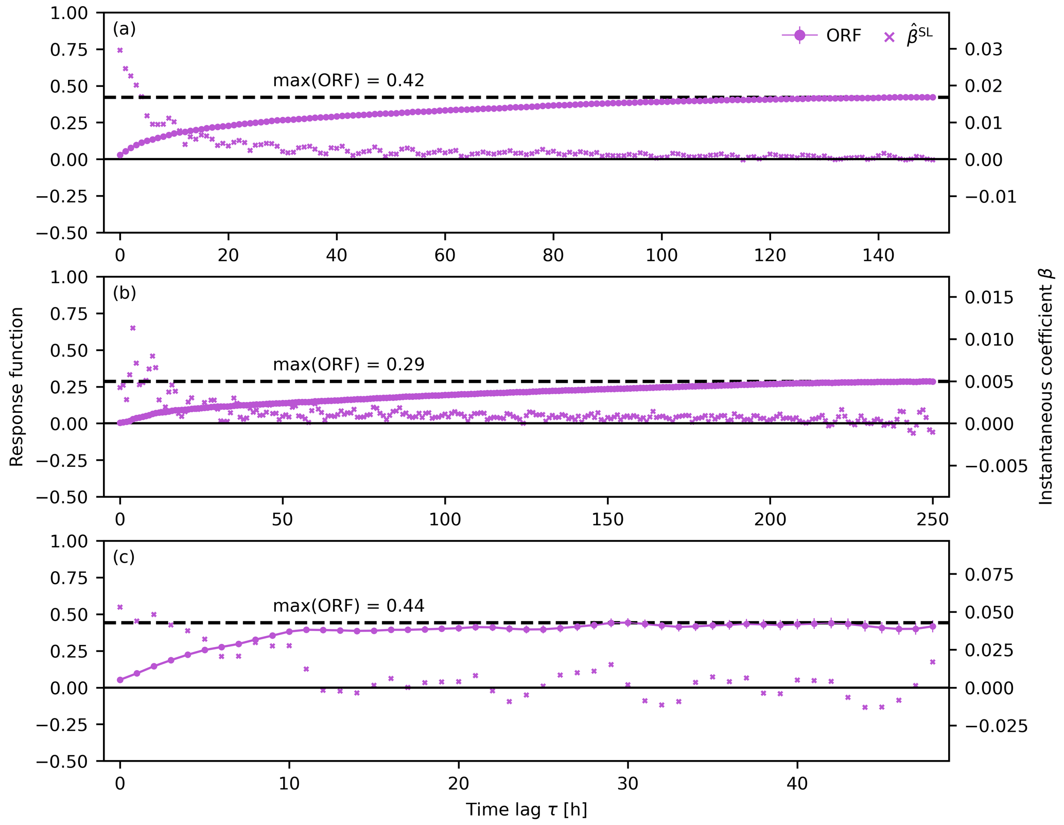
Figure 4Oceanic response function (ORF) for (a) BS3, (b) NY-10, and (c) SN12/1, with corresponding instantaneous coefficients . Note the different maximum time lag for each well on the x axis. Vertical error bars indicate an uncertainty of 1 standard error for the oceanic response function (Appendix B).
3.4 Response functions
Figure 4 shows the instantaneous coefficients and their cumulative sum that represents the oceanic response function (ORF). The coefficients are largest for small time lags and approach zero at longer lag times. Note that values should approach zero as they approach the memory of the system (i.e., sea-level changes no longer influence groundwater levels). Also note that each well has a unique ORF which can also vary with time as a result of the temporally variable characteristics of the sea-level influence (Brookfield et al., 2017). Similarly to the river-stage response function used by Spane and Mackley (2011), this memory should be longer for locations further from the source. The ORF is greater for stronger influences than for weaker influences, which is also a function of the distance from the shoreline. Similarly to the river-stage response function, the ORF is a function of aquifer hydraulic diffusivity, shoreline distance, beach sediment composition, borehole storage, and well-skin effects (Spane and Mackley, 2011).
The maximum lag time (i.e., memory) also varies by well, with 150 and 250 h for BS3 and NY-10, respectively, which reflects the greater distance from the shoreline of NY-10. The ORF stabilizes to maximum values of 0.42 and 0.29 for BS3 and NY-10, respectively (Fig. 4a and b), again reflecting the distance from the shoreline. The harmonic least-squares (HALS) analysis applied to corrected time series with different sea-level memories suggests that ocean tides are removed with small lags, and longer lags are required for aperiodic events (Appendix C).
Besides the distance from the coast and aquifer hydraulic properties, the characteristics of the sea-level fluctuations within the analyzed time period are relevant to the shape of the ORF (Brookfield et al., 2017). For Norderney, the most prominent change in sea-level characteristics is the presence of storm floods during the winter half-year and the general lack of them during the summer, as well as the generally higher variability of non-tidal sea-level components during winter and autumn (trend line in Fig. 3a). Figure 5 shows ORFs calculated for 182.5 and 73 d subsets (with different starting dates) of the 1-year time series (time frames covered are indicated in Fig. 3a and c). The ORFs are relatively close in shape to the ORF of the entire time series when winter and/or autumn are covered; i.e., they cover either the start or end of the 1-year period. When no time frame with pronounced variability in the non-tidal sea-level component is covered, the maximum ORF value tends to be smaller than that of the entire time series (orange line in Fig. 5b, Figs. S1–S9 in the Supplement), which resembles the then weaker influence of sea-level fluctuations on the groundwater levels (see Appendix D for more details). This is not observed for the 182.5 d time series as they always cover a time frame with pronounced non-tidal sea-level variability.
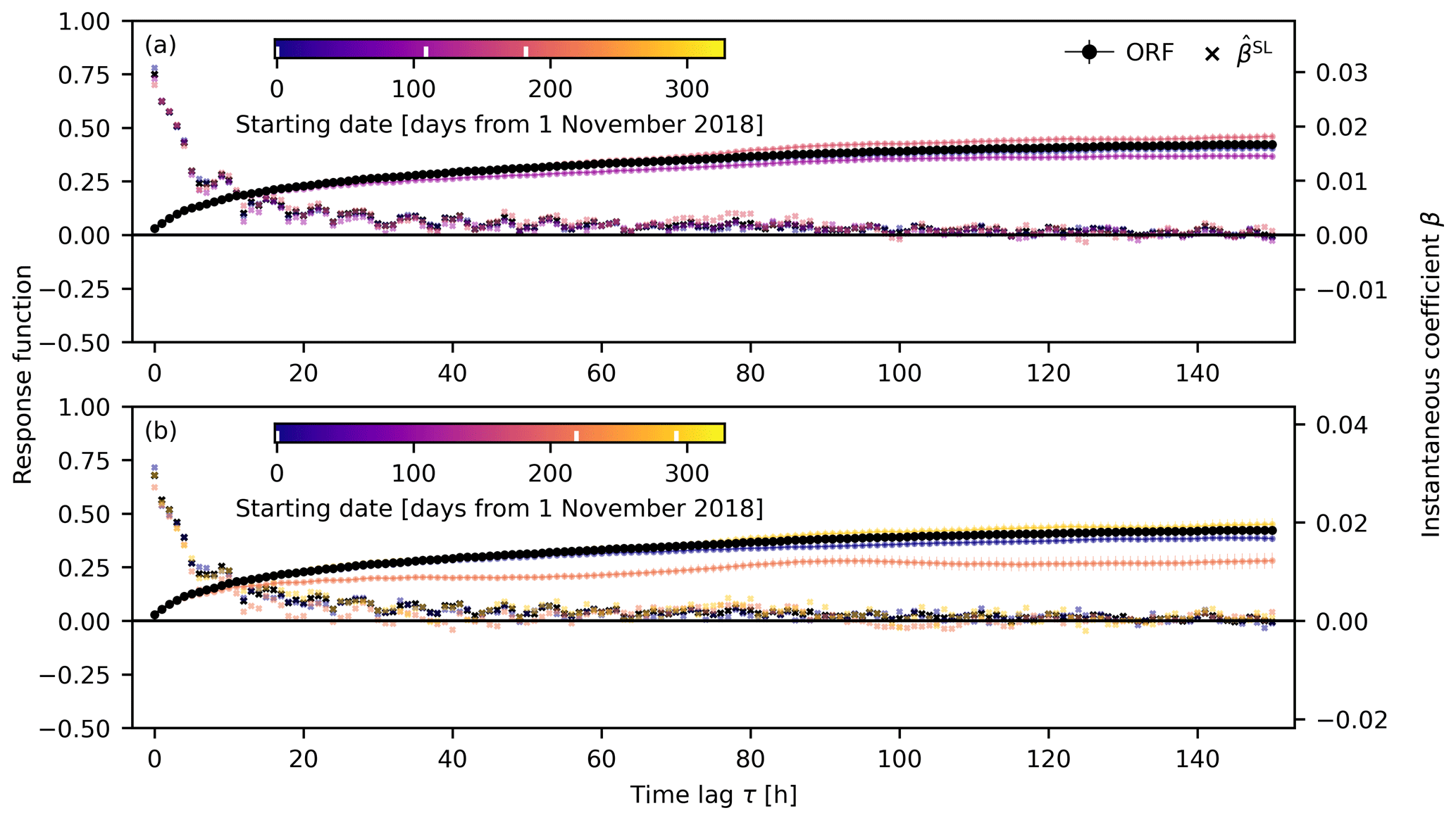
Figure 5Oceanic response function (ORF) for BS3 with time series lengths of (a) 182.5 d and (b) 73 d. The black response functions and instantaneous coefficients show the results of the analysis of the complete 1-year time series (Fig. 4a). Colors indicate the time difference of the starting point of the shorter time series compared to the starting point of the complete time series. Note that not all analyzed response functions are shown (cf. to Figs. S5 and S8). The starting dates of the analyzed time series are displayed by white stripes in the color bars. Time frames covered by the time series corresponding to the ORFs shown are displayed in matching colors in Fig. 3a and c.
In the case of the 73 d time series starting in early June 2019 (orange line in Fig. 5b), sea levels show no pronounced variation besides ocean tides (Fig. 3a). Accordingly, the instantaneous coefficients start fluctuating around zero earlier than for the other time series (Fig. 5b), indicating a shorter memory mSL of around 48 h. In conclusion, the ORF seems to be time invariant as long as the characteristics of the stresses covered by the individual time series are comparable.
Note that, generally, the maximum number of time lags (i.e., number of instantaneous coefficients) used in the regression deconvolution should only constitute a small portion of the number of time steps present in the analyzed time series to avoid overfitting. Thus, systems with longer memory require longer time series to produce meaningful response functions. In our case, for example, the longest required memory of 250 h is around 3 % of the 1-year time series.
The barometric response functions (BRFs) for BS3 and NY-10 deliver small values, and instantaneous coefficients start fluctuating around zero for τ>0 h for BS3 and τ>4 h for NY-10 (Fig. 6a and b). Thus, the response to barometric-pressure changes is instantaneous (smaller than the measurement interval, BS3) or relatively fast (NY-10). This is consistent with shallow water tables and high air permeabilities in the sandy surficial deposits that promote rapid equilibration of aquifer heads (cf. average depth to water table in Table 1) (Rasmussen and Crawford, 1997).
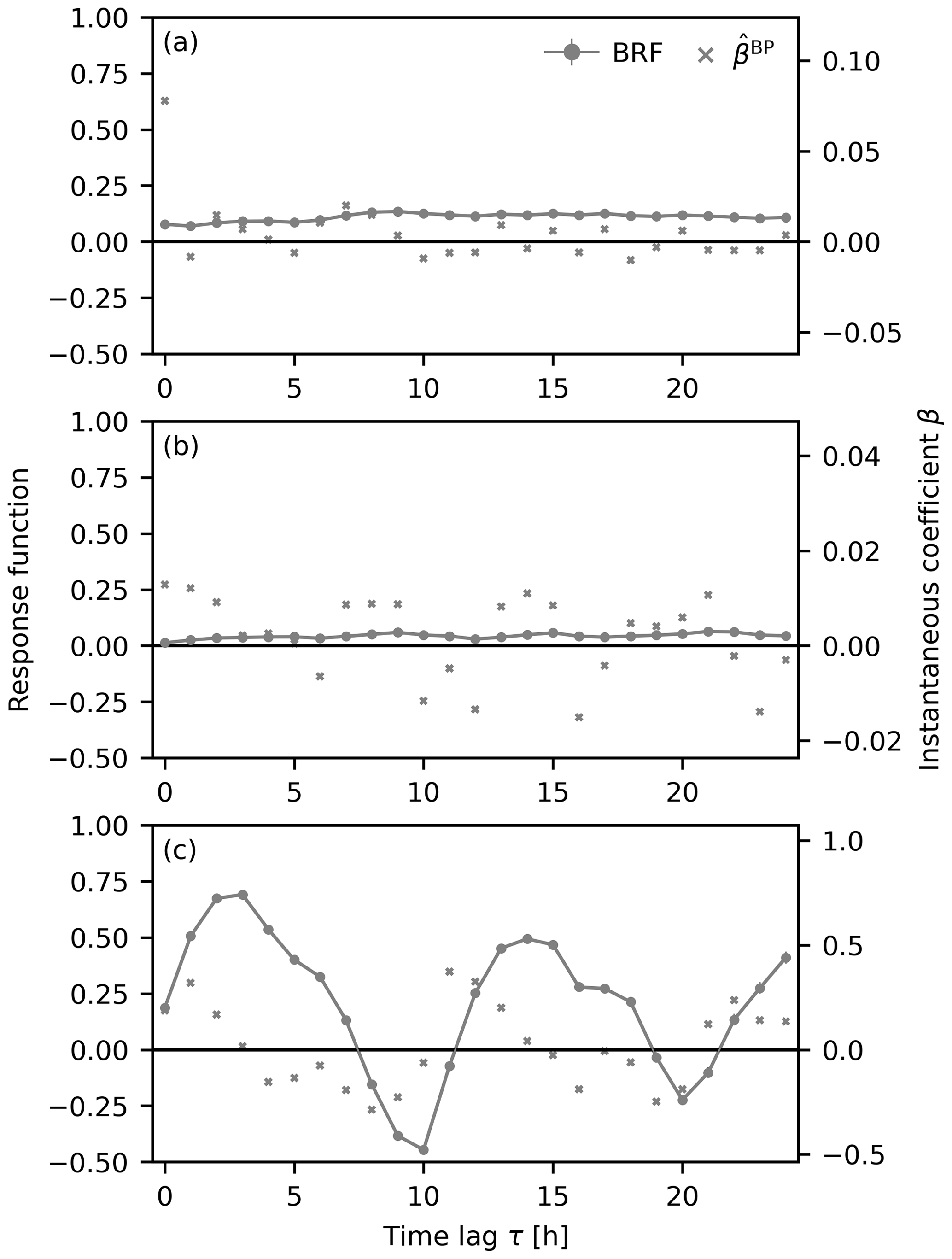
Figure 6Barometric response functions (BRFs) for (a) BS3, (b) NY-10, and (c) SN12/1 with corresponding instantaneous coefficients βBP. Vertical error bars indicate an uncertainty of 1 standard error for the barometric response function (Appendix B).
Well SN12/1 shows a faster response to sea-level changes, and the maximum ORF of 0.44 is attained within 2 d (Fig. 4c), which can be explained by the presence of the nearby confining unit (Fig. 2c). However, corrected groundwater levels still show periodic fluctuations (Fig. 3e) that HALS analysis identified as a diurnal pattern associated with the S1 tidal constituent that is not removed by deconvolution because it is not present in sea-level observations (Fig. C2c). This S1 response may be due to meteorological (e.g., evapotranspiration) or other (e.g., groundwater extraction) influences that vary at this frequency (see Sect. 3.5). Further, the BRF of SN12/1 shows a pronounced periodic pattern at ca. 2 cpd.
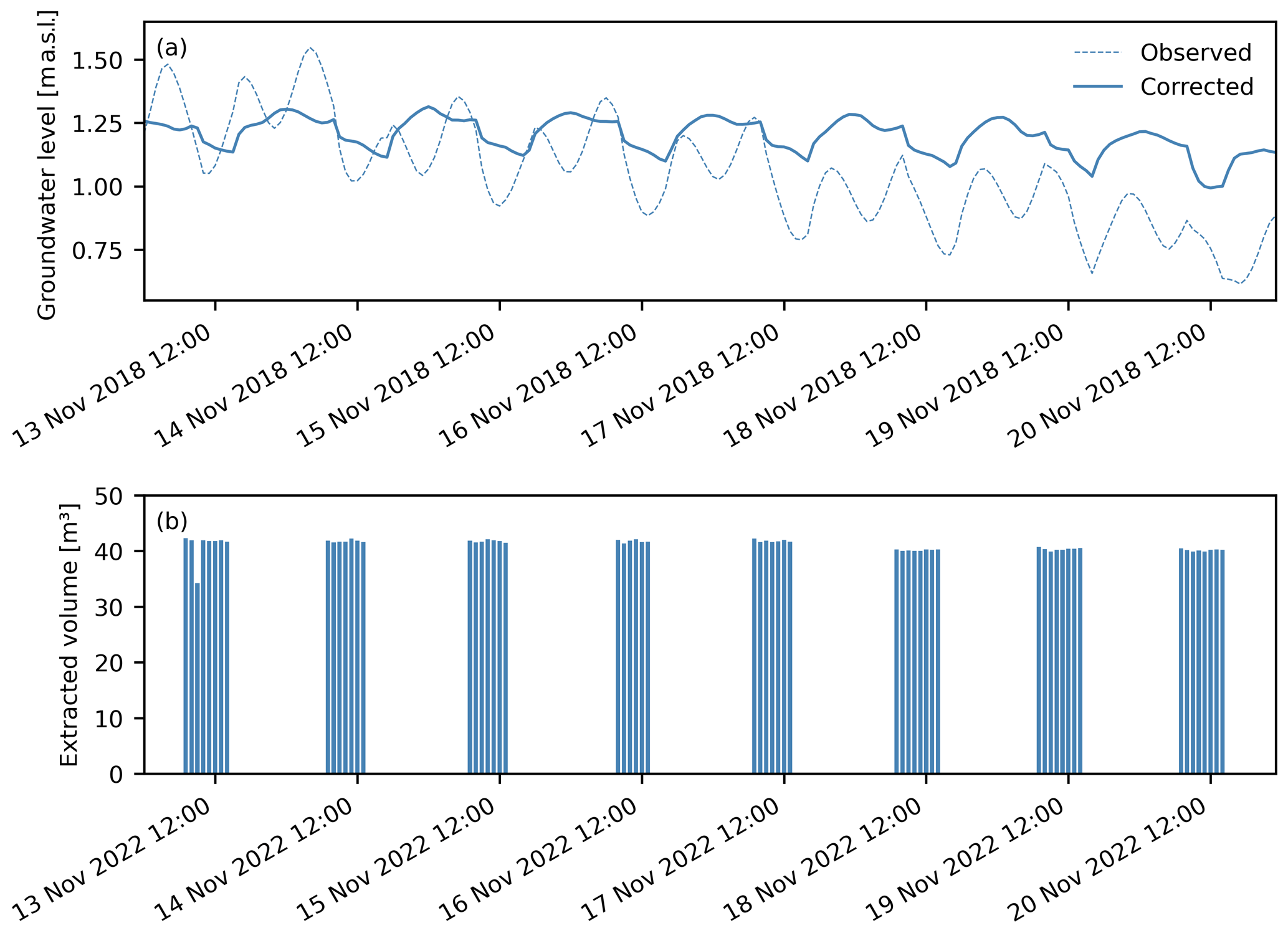
Figure 7Time series of (a) observed and corrected groundwater levels of SN12/1 and (b) extracted groundwater volume of the production wells around SN12/1 for an 8 d time period. Note that the years of both time series differ since no hourly extraction data were available for the studied time frame. However, overall groundwater extraction patterns over a season have been generally stable and comparable since the early 2000s (Stadtwerke Norderney, 2021b) so that a main extraction time period between 07:00 and 15:00 UTC+1 is very likely for 2018 as well.
3.5 Revealing groundwater extraction and aquifer-generated tidal constituents
Figure 7 shows an 8 d window in November 2018 of observed and sea-level-corrected groundwater levels from SN12/1. While the influence of groundwater extraction was masked by sea-level influences, it is clearly present after correction. Groundwater declines in the corrected time series coincide with daily extraction. This explains the visible mixed-tide type present in observed groundwater levels that cannot originate from the semi-diurnal, M2-dominated ocean tide, with only small diurnal components (see Fig. C1).
We compare this pattern with groundwater extraction data from 2022, which show that pumping patterns are similar to corrected groundwater levels. We rely on 2022 extraction data because such data were not available during the study period. Also, seasonal extraction patterns and yearly extraction volumes have remained stable since the early 2000s (Stadtwerke Norderney, 2021b). The strong coherence between these two time series provides further evidence for the utility of regression deconvolution in removing interference from external stimuli.
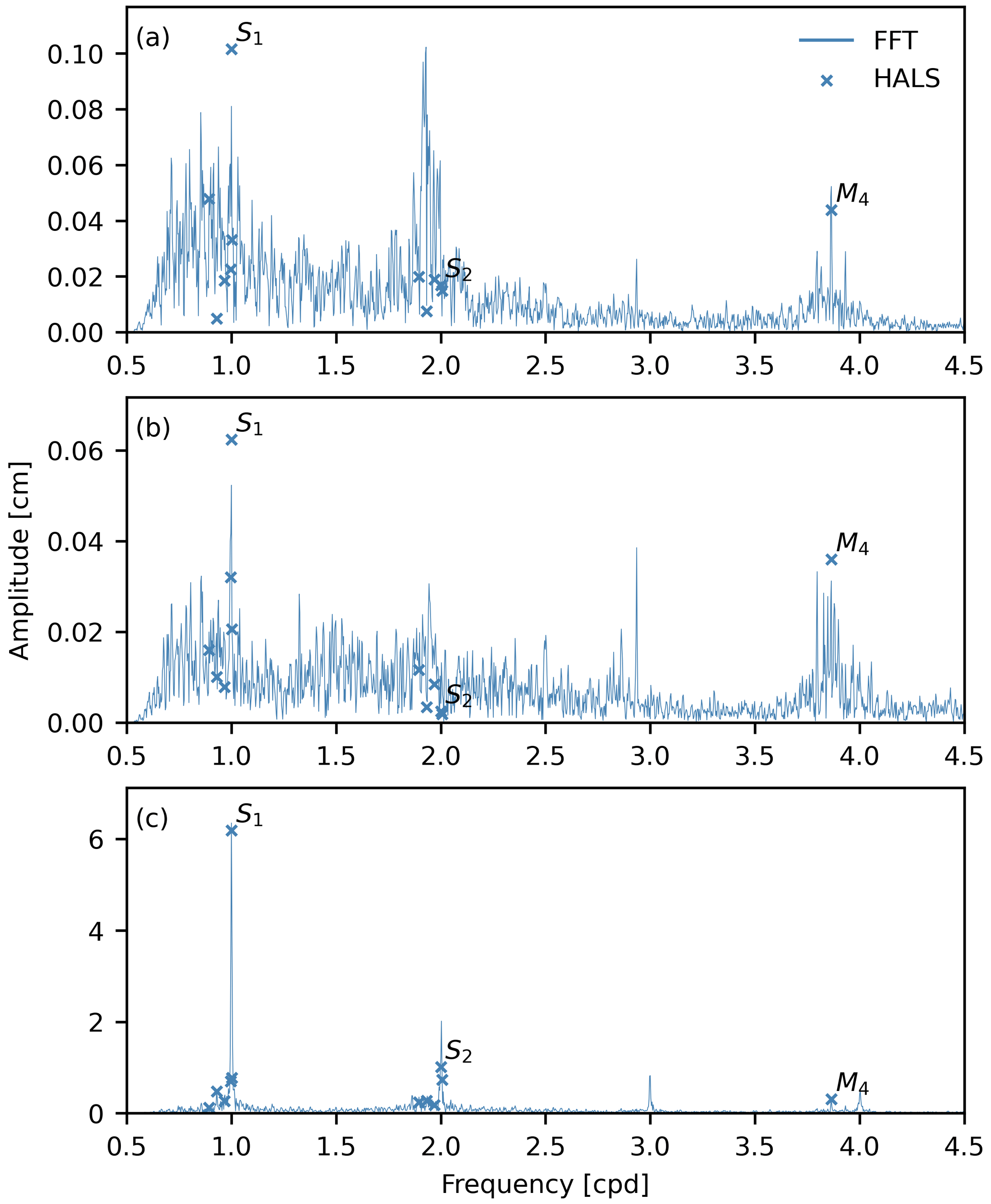
Figure 8Amplitudes found in the corrected groundwater-level time series for frequencies between 0.5 and 4.5 cpd obtained with harmonic least-squares (HALS) analysis and a fast Fourier transform (FFT) for (a) BS3, (b) NY-10, and (c) SN12/1. The HALS data show tidal constituents as outlined in Fig. C1. Note the different y axis scales on each panel.
While the pattern of groundwater extraction is clearly visible in the groundwater-level time series of SN12/1, this influence is also present at monitoring wells BS3 and NY-10. To show this, amplitudes of frequencies between 0 and 12 cpd were extracted from the corrected groundwater-level time series using HALS analysis (see Appendix C) and the fast Fourier transform (FFT) with a Hanning window (Fig. 8). This shows that the daily groundwater extraction pattern strongly enhances the S1 tidal constituent at SN12/1 to around 6 cm (Fig. 8c) compared to an amplitude of around 0.8 cm present in the ocean-tide signal (Fig. C1). For BS3 and NY-10, the amplitude of the tidal constituent S1 introduced by groundwater extraction is much smaller due to the larger distance to the production wells (Fig. 8a and b).
The groundwater extraction signal is one of the causes of the small-amplitude, high-frequency oscillations remaining in the corrected groundwater-level time series (Fig. 3a and b) and the oscillation visible in the instantaneous coefficients of the regression deconvolution (at ca. 4 cpd; see Fig. 4a and b) of BS3 and NY-10. The second source of the oscillations is the generation of the shallow-water tidal constituent M4 within the aquifer as a result of the propagation of the tidal signal in the sediment (Bye and Narayan, 2009, see Sect. 3.3). It is generated as the higher harmonic of the M2 constituent, which is the dominating tidal constituent at the study site (Fig. C1), so that the amplitude and phase lag of the generated M4 constituent depend on the amplitude and phase lag of the ocean-tide M2 constituent (Bye and Narayan, 2009). For the large amplitude of the ocean-tide M2 constituent (Fig. C1), the amplitude of the generated M4 constituent is still discernible from noise in the data at the monitoring wells (Fig. 8). Further, there is noise present in the corrected time series for frequencies between 0.5 and 3 cpd which cannot be attributed to major tidal constituents (Fig. 8), but parts of it may be attributed to the frequency-dependent amplitude attenuation and phase shift of the different tidal constituents within the aquifer sediment (see Sect. 3.3).
The oscillating BRF of SN12/1 (Fig. 6c) is likely to be a result of the groundwater extraction signal not being present in the regression deconvolution. A similar pattern was observed by Patton et al. (2021) in their analysis of the barometric pressure and Earth tide response of groundwater levels in a coastal aquifer in relation to ocean tides (they termed this shape “peaked”). In their study, they did not consider sea-level fluctuations and the semi-diurnal ocean-tide pattern mapped to the BRF. The oscillation in the BRF of SN12/1 is likely to be mixed semi-diurnal and diurnal because the tidal constituents S1 and S2 introduced by groundwater extraction are not removed at the given memory mSL=48 h (Fig. C2c).
We demonstrate how regression deconvolution can be used to remove sea-level influences from groundwater levels measured in coastal aquifers, which has not been illustrated before. We define and use an oceanic response function (ORF) to represent the time-lag-dependent response coefficients for characterizing groundwater responses to sea-level changes. Once sea-level influences have been removed, the resulting groundwater levels clearly show previously masked responses to precipitation and groundwater extraction. In this application, the horizontal propagation of sea-level changes dominates groundwater responses.
Our findings expand the range of applications for regression deconvolution by enabling the characterization and mitigation of external perturbations impacting groundwater levels. These perturbations encompass barometric pressure; Earth tide; river stage fluctuations; and, now, oceanic influences. Our methodology is well-suited for analyzing data obtained from groundwater monitoring in oceanic and coastal aquifers. This capability is instrumental in enhancing our understanding and sustainable management of these critical water systems. Future research endeavors should prioritize a systematic exploration of how hydraulic processes (e.g., modulation of tidal signals within aquifer sediments) and properties (e.g., hydraulic diffusivity) in coastal aquifers affect oceanic response functions. Additionally, estimating response functions linked to groundwater extraction will become an important area for investigation once suitable data become available.
The ORF shapes depend on the stresses present in the sea-level time series and are only similar for different time frames, i.e., time invariant, when the stresses of the time frames are similar. A time frame containing storm events may yield a different ORF than a time frame were ocean tides are the most prominent sea-level influence. In the case of Norderney, the assumption of a linear response of groundwater levels to sea-level influences will likely be approximately valid, resulting from the small changes in saturated aquifer thickness introduced by the sea-level fluctuations (Reilly et al., 1987; Smith, 2008).
While many hydrogeological settings will likely require the estimation of other effects (e.g., Earth tides, soil moisture, river stage), we neglect these influences at this site due to their minimal influence. Regardless of the specific application, however, our methodology for removing multiple factors should provide sufficient flexibility for interpreting and removing these influences.
The hourly barometric time series data from the meteorological station on Norderney were compared to data from the stations of Wittmund (ca. 39 km from Norderney) on the mainland (DWD Climate Data Center, 2023b) and Leuchtturm Alte Weser (ca. 66 km from Norderney) in the German Wadden Sea (DWD Climate Data Center, 2023a) (Fig. 2b). Figure A1 shows the data of these stations plotted against the data from Norderney and the results of a linear regression analysis performed on these data sets. Data from Norderney and Wittmund are very similar, with only little offset, while the data from Leuchtturm Alte Weser are offset from data from Norderney by around 6 cm H2O. Cross-correlation analysis shows the largest cross-correlations between Norderney station and Wittmund at a time lag of 0 h and for Leuchtturm Alte Weser at a time lag of 2 h. Due to the similarities of the data collected at these stations, which have spatial differences of tens of kilometers, we assume that spatial variability in barometric pressure at the scale of the study area is negligible.
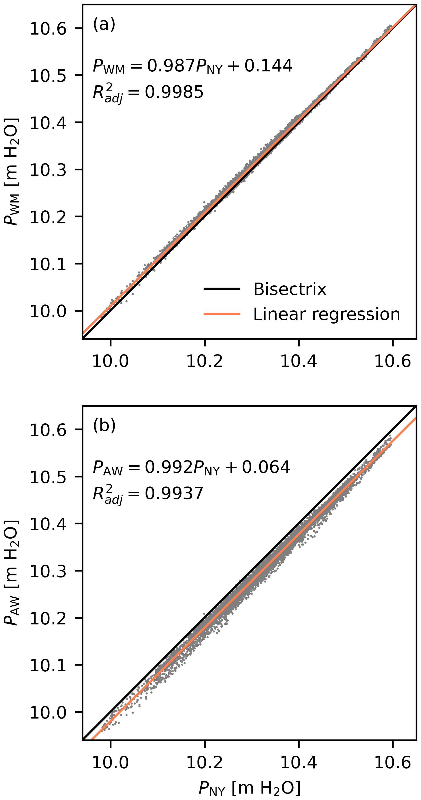
Figure A1Comparison of barometric-pressure (P) data collected at the meteorological station on Norderney (PNY) and at (a) Wittmund (PWM) and (b) Leuchtturm Alte Weser (PAW) (cf. Fig. 2b). Shown are results of a linear regression analysis performed on the data as well.
The sea-level data with 1 min time increments from the tide gauge Norderney Riffgat were compared to sea-level data from the tide gauge Spiekeroog (WSV, 2021b) to assess the time shift of the tidal signal to be expected along the shoreline of the islands (Fig. 2b). The tide gauge on Spiekeroog is located approximately 35 km east of the tide gauge on Norderney (Fig. 2b) and should thus lag behind the time series observed on Norderney (Malcherek, 2010). Cross-correlation analysis of the sea-level time series from Norderney and Spiekeroog shows the maximum correlation at a time lag of 33 min. Thus, the sea-level signal observed on Spiekeroog commonly lags behind the signal observed on Norderney by ca. half an hour. In conclusion, the temporal offset between the tide gauge Norderney Riffgat and the shoreline segments close to the groundwater observation wells can be expected to be on the order of a few minutes.
The standard error SEORF(τk) of the ORF at time lag τk is calculated from the [mSL×mSL] covariance matrix σ for the instantaneous coefficients βSL obtained by regression deconvolution:
where σii is the variance of instantaneous coefficients at time lag τi, and σij is the covariance at lags τi and τj. The same procedure applies to the BRF.
Amplitudes and phases of major tidal constituents (see e.g., McMillan et al., 2019) were obtained from sea-level and groundwater-level time series using harmonic least-squares (HALS) analysis (for an outline of HALS, see, e.g., Schweizer et al., 2021). Barometric pressure was only analyzed for the subset of tidal constituents relevant to atmospheric tides (Rau et al., 2020). Amplitude and phase uncertainties were estimated as described in Appendix C of Rau et al. (2020).
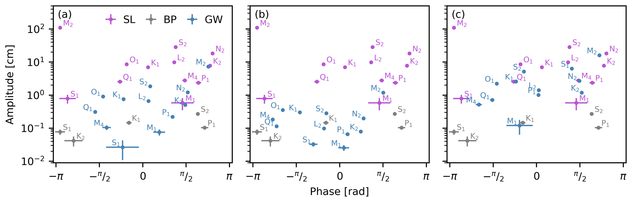
Figure C1Amplitudes and phases obtained using harmonic least-squares (HALS) analysis of groundwater-level (GW) time series of monitoring wells (a) BS3, (b) NY-10, and (c) SN12/1. Each plot shows the HALS analysis for sea level (SL) and barometric pressure (BP). Error bars show uncertainty of 1 standard error.
Results of the HALS analysis are shown in Fig. C1 and identify the semi-diurnal characteristic of the ocean tides with only minor diurnal constituents. This pattern is retained in the groundwater response for BS3 and NY-10 (Fig. C1a and b), but the principal diurnal solar constituent S1 is amplified compared to the sea-level signal in the data observed at SN12/1, which indicates that parts of the spectral power present at this frequency must originate from another process (compare Sect. 3.5).
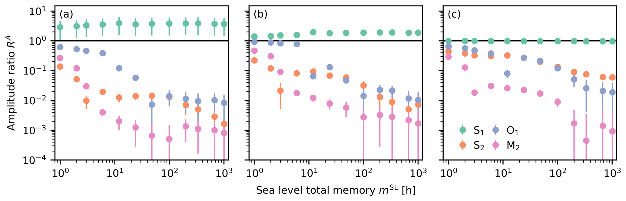
Figure C2Amplitude ratios of observed and corrected groundwater levels (Eq. C1) for tidal constituents obtained by the harmonic least-squares (HALS) analysis performed on (a) BS3, (b) NY-10, and (c) SN12/1 as a function of the sea-level memory (mSL). Error bars show uncertainty of 1 standard error.
Figure C2 shows the amplitude ratio,
between the amplitudes of tidal constituent ν in the observed () and corrected () groundwater time series for different sea-level memories mSL between 1 h and 6 weeks. Uncertainties are shown as standard errors,
obtained by propagating amplitude uncertainties estimated using HALS.
Semi-diurnal constituents, like M2 or S2, are easily removed. A maximum lag of around 6 h suffices for reducing the amplitudes in BS3 and NY-10 to below approximately 5 % to 10 % of their original values (Fig. C2a and b). However, this is only the case for M2 in SN12/1 (Fig. C2c). Diurnal constituents like O1 require larger total memory of around 12 to 24 h to be reduced equally well (Fig. C2). However, a successful removal of O1 can be assumed for larger amplitude ratios considering the smaller absolute amplitude in the observed signal compared to the semi-diurnal constituents (Fig. C1).
The S1 tidal constituent is not removed from the groundwater signal and is actually larger in the corrected groundwater signal than in the observed signal in BS3 and NY-10 (Fig. C2a and b). Yet, this constituent has little overall effect due to its minor amplitude (Fig. C1a and b). As noted in Sect. 3.5, corrected groundwater levels in SN12/1 contain daily signals from nearby production wells. Figure C2c shows that this diurnal pattern maps to S1. The amplification of S1 for BS3 and NY-10 in the corrected time series likely has the same origin and could be caused by the removal of an interference between the ocean tide's S1 and the daily extraction signal in the observed data.
The oceanic response function (ORF) was calculated for smaller portions of the time series from 1 November 2018 to 31 October 2019 to check the dependence of the results on the length of the time series. Analyzed time series lengths were 328.5 d (90 % of the original time series, n=2 samples with different starting points), 292 d (80 %, n=3), 255.5 d (70 %, n=4), 219 d (60 %, n=5), 182.5 d (50 %, n=6), 146 d (40 %, n=7), 109.5 d (30 %, n=8), 73 d (20 %, n=9), and 36.5 d (10 %, n=10). The starting time points of the time series were defined every 36.5 d from 1 November 2018 onwards. The ORF memory mSL of 150 h for BS3, 250 h for NY-10, and 48 h for SN12-1 and the BRF memory mBP of 24 h for all monitoring wells were kept unchanged for the analysis. All calculated ORFs are displayed in Figs. S1–S9.
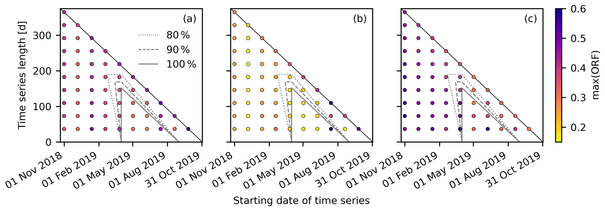
Figure D1Maximum values of the oceanic response function (max(ORF)) as a function of the starting date of the time series and the time series length for (a) BS3, (b) NY-10, and (c) SN12-1. Contour lines indicate the percentage of a time series within the time frame from 1 April to 31 August 2019, where the non-tidal sea-level changes are small (see Fig. 3a). Only the lower triangles of the plots are filled as, in the upper ones, time series would exceed the end of the studied time frame on 31 October 2019. Bounds of the color bar are the 5th and 95th percentiles of all max(ORF) values shown in this figure.
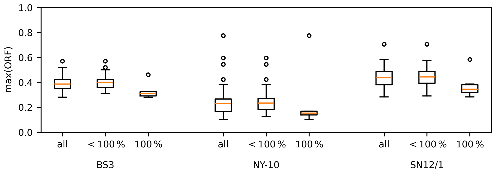
Figure D2Distribution of the maximum values of the oceanic response function (max(ORF)) for the three monitoring wells. Shown are boxplots for all time series shown in Fig. D1 (“all”), for time series which are not entirely within the time frame from 1 April to 31 August 2019 (“<100 %”), and for time series completely within this time frame (“100 %”).
The maximum value of the ORF depends on the length of the time series and the time frame covered (Fig. D1). Especially for BS3 and NY-10, there also seems to be a dependence on the starting date of the time series, independent of the time series length (Fig. D1a and b). For SN12/1, there seems to be a stronger interdependence between the starting time point and the time series length, where shorter time series that have an earlier starting date show the largest max(ORF) values.
For all three monitoring wells, the max(ORF) values are generally smaller when a time series only covers the time frame from 1 April to 31 August 2019, where non-tidal sea-level variability is smaller than in winter and autumn (Fig. D2; see Fig. 3a). This effect is less pronounced at NY-10 because it is further from the shore; thus, the non-tidal sea-level changes have less effect on the groundwater levels at this location (Fig. 3d).
Python scripts and data used in this work are available on Zenodo under https://doi.org/10.5281/zenodo.10868409 (Haehnel and Rau, 2023). An online application (MUFACO: multi-factor correction of groundwater levels) to calculate multi-factor regression deconvolution and to obtain response functions for multiple stressors is available at https://groundwater.app/app-mufaco/ (Rau, 2023).
The supplement related to this article is available online at: https://doi.org/10.5194/hess-28-2767-2024-supplement.
PH – formal analysis, data curation, software, visualization, writing – original draft, writing – review and editing. TCR – methodology, formal analysis, supervision, writing – original draft, writing – review and editing. GCR – conceptualization, methodology, software, supervision, writing – original draft, writing – review and editing.
The contact author has declared that none of the authors has any competing interests.
Publisher's note: Copernicus Publications remains neutral with regard to jurisdictional claims made in the text, published maps, institutional affiliations, or any other geographical representation in this paper. While Copernicus Publications makes every effort to include appropriate place names, the final responsibility lies with the authors.
We thank the Stadtwerke Norderney (Municipal Works Norderney), especially Oliver Rass, for providing groundwater data and support, as well as for approving the publication of these data in the Zenodo repository. We give thanks to the Wasser- und Schifffahrtsverwaltung des Bundes (German Federal Waterways and Shipping Administration) and the Bundesamt für Gewässerschutz (German Federal Institute of Hydrology) for providing the tide gauge data. Further, we thank the two reviewers for their constructive comments which helped to improve the paper significantly.
Research for this work was funded by the German Federal Ministry of Education and Research (BMBF, Bundesministerium für Bildung und Forschung; project “Water at the Coasts of East Frisia, WAKOS”, funding reference no. 01LR2003E). This technical note was published with the help of the DFG-funded Open Access Publication Fund of the Carl von Ossietzky University Oldenburg.
This paper was edited by Monica Riva and reviewed by Rachel Housego and one anonymous referee.
Bakker, M. and Schaars, F.: Solving Groundwater Flow Problems with Time Series Analysis: You May Not Even Need Another Model, Groundwater, 57, 826–833, https://doi.org/10.1111/gwat.12927, 2019. a, b
Barlow, P. M.: Ground water in freshwater-saltwater environments of the Atlantic coast, Circular 1262, US Geological Survey, Reston, https://doi.org/10.3133/cir1262, 2003. a
Boon, J. D.: Secrets of the Tide: Tide and Tidal Current Analysis and Applications, Storm Surges and Sea Level Trends, Woodhead Publishing, Cambridge, https://doi.org/10.1016/B978-1-904275-17-6.50011-2, 2011. a, b
Brookfield, A. E., Stotler, R. L., and Reboulet, E. C.: Interpreting Temporal Variations in River Response Functions: An Example from the Arkansas River, Kansas, USA, Hydrogeol. J., 25, 1271–1282, https://doi.org/10.1007/s10040-017-1545-9, 2017. a, b
Butler Jr., J. J., Jin, W., Mohammed, G. A., and Reboulet, E. C.: New Insights from Well Responses to Fluctuations in Barometric Pressure, Groundwater, 49, 525–533, https://doi.org/10.1111/j.1745-6584.2010.00768.x, 2011. a, b, c
Bye, J. A. and Narayan, K. A.: Groundwater response to the tide in wetlands: Observations from the Gillman Marshes, South Australia, Estuar. Coast. Shelf Sci., 84, 219–226, https://doi.org/10.1016/j.ecss.2009.06.025, 2009. a, b, c
Cartwright, N., Baldock, T. E., Nielsen, P., Jeng, D.-S., and Tao, L.: Swash-aquifer interaction in the vicinity of the water table exit point on a sandy beach, J. Geophys. Res., 111, C09035, https://doi.org/10.1029/2005JC003149, 2006. a
Collenteur, R. A., Bakker, M., Caljé, R., Klop, S. A., and Schaars, F.: Pastas: Open Source Software for the Analysis of Groundwater Time Series, Groundwater, 57, 877–885, https://doi.org/10.1111/gwat.12925, 2019. a, b
Collenteur, R. A., Bakker, M., Klammler, G., and Birk, S.: Estimation of groundwater recharge from groundwater levels using nonlinear transfer function noise models and comparison to lysimeter data, Hydrol. Earth Syst. Sci., 25, 2931–2949, https://doi.org/10.5194/hess-25-2931-2021, 2021. a
DWD Climate Data Center – CDC: Historical daily station observations (temperature, pressure, precipitation, sunshine duration, etc.) for Norderney (station 3631), version v006, DWD – Deutscher Wetterdienst [German Meteorological Service] [data set], https://opendata.dwd.de/climate_environment/CDC/observations_germany/climate/daily/kl/historical/ (last access: 29 March 2021), 2021a. a, b, c
DWD Climate Data Center – CDC: Historical hourly station observations of precipitation for Norderney (station 3631) from 1949 to 2020, version v21.3, DWD – Deutscher Wetterdienst [German Meteorological Service] [data set], https://opendata.dwd.de/climate_environment/CDC/observations_germany/climate/hourly/precipitation/historical/ (last access: 1 October 2021), 2021b. a, b
DWD Climate Data Center – CDC: Historical hourly station observations of pressure for Norderney (station 3631) from 1949 to 2020, version v21.3, DWD – Deutscher Wetterdienst [German Meteorological Service] [data set], https://opendata.dwd.de/climate_environment/CDC/observations_germany/climate/hourly/pressure/historical/ (last access: 1 October 2021), 2021c. a, b
DWD Climate Data Center – CDC: Historical hourly station observations of pressure for Leuchtturm Alte Weser (Station 0102) from 1949 to 2022, version v23.3, DWD – Deutscher Wetterdienst [German Meteorological Service] [data set], https://opendata.dwd.de/climate_environment/CDC/observations_germany/climate/hourly/pressure/historical/ (last access: 23 August 2023), 2023a. a
DWD Climate Data Center – CDC): Historical hourly station observations of pressure for Wittmund (Station 5640) from 1949 to 2022, version v23.3, DWD – Deutscher Wetterdienst [German Meteorological Service] [data set], https://opendata.dwd.de/climate_environment/CDC/observations_germany/climate/hourly/pressure/historical/ (last access: 23 August 2023), 2023b. a
EuroGeographics and UN-FAO: Countries, 2020 – Administrative Units, 1:1 000 000, provided by Eurostat [data set], https://ec.europa.eu/eurostat/web/gisco/geodata/reference-data/administrative-units-statistical-units/countries (last access: 29 November 2021), 2020. a
Falkland, A. (Ed.): Hydrology and water resources of small islands: a practical guide, no. 49, in: Studies and reports in hydrology, UNESCO, Paris, ISBN 92-3-102753-0, 1991. a
Ferris, J. G.: Cyclic fluctuations of water level as a basis for determining aquifer transmissibility, USGS Unnumbered Series Note 1, US Geological Survey, Washington, D.C., https://doi.org/10.3133/70133368, 1952. a
Furbish, D. J.: The response of water level in a well to a time series of atmospheric loading under confined conditions, Water Resour. Res., 27, 557–568, https://doi.org/10.1029/90WR02775, 1991. a
Gomes da Silva, P., Coco, G., Garnier, R., and Klein, A. H.: On the prediction of runup, setup and swash on beaches, Earth-Sci. Rev., 204, 103148, https://doi.org/10.1016/j.earscirev.2020.103148, 2020. a, b, c
Gönnert, G.: Sturmfluten und Windstau in der Deutschen Bucht - Charakter, Veränderungen und Maximalwerte im 20. Jahrhundert, Die Küste, 67, 185–365, 2003. a
Greskowiak, J. and Massmann, G.: The impact of morphodynamics and storm floods on pore water flow and transport in the subterranean estuary, Hydrol. Process., 35, e14050, https://doi.org/10.1002/hyp.14050, 2021. a
Grünenbaum, N., Günther, T., Greskowiak, J., Vienken, T., Müller-Petke, M., and Massmann, G.: Salinity distribution in the subterranean estuary of a meso-tidal high-energy beach characterized by Electrical Resistivity Tomography and direct push technology, J. Hydrol., 617, 129074, https://doi.org/10.1016/j.jhydrol.2023.129074, 2023. a
Haehnel, P. and Rau, G. C.: Workflow, scripts, and data for technical note “Removing dynamic sea-level influences from groundwater-level measurements” (Version 1.2.0), Zenodo [code and data set], https://doi.org/10.5281/zenodo.10868409, 2023. a
Haehnel, P., Freund, H., Greskowiak, J., and Massmann, G.: Development of a three-dimensional hydrogeological model for the island of Norderney (Germany) using GemPy, Geosci. Data J., https://doi.org/10.1002/gdj3.208, online first, 2023. a, b, c, d
Hayes, M. O.: Barrier Island Morphology as a Function of Tidal and Wave Regime, in: Barrier Islands from the Gulf of St. Lawrence to the Gulf of Mexico, edited by: Leatherman, S. P., Academic Press, New York, 1–29, ISBN 9780124402607, 1979. a
Hegge, B. J. and Masselink, G.: Groundwater-Table Responses to Wave Run-up: An Experimental Study From Western Australia, J. Coast. Res., 7, 623–634, 1991. a
Holt, T., Greskowiak, J., Seibert, S. L., and Massmann, G.: Modeling the Evolution of a Freshwater Lens under Highly Dynamic Conditions on a Currently Developing Barrier Island, Geofluids, 2019, 9484657, https://doi.org/10.1155/2019/9484657, 2019. a
Houben, G. J., Koeniger, P., and Sültenfuß, J.: Freshwater lenses as archive of climate, groundwater recharge, and hydrochemical evolution: Insights from depth-specific water isotope analysis and age determination on the island of Langeoog, Germany, Water Resour. Res., 50, 8227–8239, https://doi.org/10.1002/2014WR015584, 2014. a
Housego, R., Raubenheimer, B., Elgar, S., Cross, S., Legner, C., and Ryan, D.: Coastal Flooding Generated by Ocean Wave- and Surge-Driven Groundwater Fluctuations on a Sandy Barrier Island, J. Hydrol., 603, 126920, https://doi.org/10.1016/j.jhydrol.2021.126920, 2021. a
Jiao, J. J. and Post, V. E. A.: Coastal Hydrogeology, Cambridge University Press, Cambridge, https://doi.org/10.1017/9781139344142, 2019. a, b
Karle, M., Bungenstock, F., and Wehrmann, A.: Holocene coastal landscape development in response to rising sea level in the Central Wadden Sea coastal region, Neth. J. Geosci., 100, e12, https://doi.org/10.1017/njg.2021.10, 2021. a
Koeniger, P., Gaj, M., Beyer, M., and Himmelsbach, T.: Review on soil water isotope-based groundwater recharge estimations, Hydrol. Process., 30, 2817–2834, https://doi.org/10.1002/hyp.10775, 2016. a
Li, L., Barry, D., and Pattiaratchi, C.: Numerical modelling of tide-induced beach water table fluctuations, Coast. Eng., 30, 105–123, https://doi.org/10.1016/S0378-3839(96)00038-5, 1997. a
Li, L., Cartwright, N., Nielsen, P., and Lockington, D.: Response of Coastal Groundwater Table to Offshore Storms, China Ocean Eng., 18, 423–431, 2004. a
Malcherek, A.: Gezeiten und Wellen, Die Hydromechanik der Küstengewässer, Vieweg+Teubner, Wiesbaden, https://doi.org/10.1007/978-3-8348-9764-0, 2010. a
McMillan, T. C., Rau, G. C., Timms, W. A., and Andersen, M. S.: Utilizing the Impact of Earth and Atmospheric Tides on Groundwater Systems: A Review Reveals the Future Potential, Rev. Geophys., 57, 281–315, https://doi.org/10.1029/2018RG000630, 2019. a, b
Naumann, K.: Eine hydrogeologische Systemanalyse von Süßwasserlinsen als Grundlage einer umweltschonenden Grundwasserbewirtschaftung, PhD thesis, Technischen Universität Carolo-Wilhelmina zu Braunschweig, Braunschweig, https://doi.org/10.24355/dbbs.084-200511080100-343, 2005. a, b, c, d, e
Nielsen, P.: Tidal dynamics of the water table in beaches, Water Resour. Res., 26, 2127–2134, https://doi.org/10.1029/WR026i009p02127, 1990. a, b
Nielsen, P.: Groundwater Dynamics and Salinity in Coastal Barriers, J. Coast. Res., 15, 732–740, 1999. a
NLWKN – Niedersächsischer Landesbetrieb für Wasserwirtschaft, Küsten- und Naturschutz [Lower Saxony Water Management, Coastal Defense and Nature Conservation Agency]: Dedicated dikes in Lower Saxony, NLWKN [data set], https://geoportal.geodaten.niedersachsen.de/harvest/srv/ger/catalog.search#/metadata/8A90C8B8-68D0-485C-9950-8964E6921244 (last access: 28 April 2022), 2021. a
Olsthoorn, T. N.: Do a Bit More with Convolution, Groundwater, 46, 13–22, https://doi.org/10.1111/j.1745-6584.2007.00342.x, 2008. a
Patton, A. M., Rau, G. C., Cleall, P. J., and Cuthbert, M. O.: Hydro-geomechanical characterisation of a coastal urban aquifer using multiscalar time and frequency domain groundwater-level responses, Hydrogeol. J., 29, 2751–2771, https://doi.org/10.1007/s10040-021-02400-5, 2021. a, b
Petersen, J., Pott, R., Janiesch, P., and Wolff, J.: Umweltverträgliche Grundwasserbewirtschaftung in hydrologisch und ökologisch sensiblen Bereichen der Nordseeküste, Husum Druck- und Verlagsgesellschaft mbH u. Co. KG., Husum, ISBN 9783898761116, 2003. a
Pezij, M., Augustijn, D. C. M., Hendriks, D. M. D., and Hulscher, S. J. M. H.: Applying transfer function-noise modelling to characterize soil moisture dynamics: a data-driven approach using remote sensing data, Environ. Model. Softw., 131, 104756, https://doi.org/10.1016/j.envsoft.2020.104756, 2020. a
Post, V., Kooi, H., and Simmons, C.: Using Hydraulic Head Measurements in Variable-Density Ground Water Flow Analyses, Ground Water, 45, 664–671, https://doi.org/10.1111/j.1745-6584.2007.00339.x, 2007. a
Post, V. E. A.: Electrical Conductivity as a Proxy for Groundwater Density in Coastal Aquifers, Ground Water, 50, 785–792, https://doi.org/10.1111/j.1745-6584.2011.00903.x, 2012. a
Post, V. E. A., Houben, G. J., and van Engelen, J.: What is the Ghijben–Herzberg principle and who formulated it?, Hydrogeol. J., 26, 1801–1807, https://doi.org/10.1007/s10040-018-1796-0, 2018. a
Post, V. E. A., Zhou, T., Neukum, C., Koeniger, P., Houben, G. J., Lamparter, A., and Šimůnek, J.: Estimation of groundwater recharge rates using soil-water isotope profiles: A case study of two contrasting dune types on Langeoog Island, Germany, Hydrogeol. J., 30, 797–812, https://doi.org/10.1007/s10040-022-02471-y, 2022. a
Rasmussen, T. C. and Crawford, L. A.: Identifying and Removing Barometric Pressure Effects in Confined and Unconfined Aquifers, Groundwater, 35, 502–511, https://doi.org/10.1111/j.1745-6584.1997.tb00111.x, 1997. a, b, c, d, e, f, g
Rasmussen, T. C. and Mote, T. L.: Monitoring Surface and Subsurface Water Storage Using Confined Aquifer Water Levels at the Savannah River Site, USA, Vadose Zone J., 6, 327–335, https://doi.org/10.2136/vzj2006.0049, 2007. a, b, c
Rau, G. C., Cuthbert, M. O., Acworth, R. I., and Blum, P.: Technical note: Disentangling the groundwater response to Earth and atmospheric tides to improve subsurface characterisation, Hydrol. Earth Syst. Sci., 24, 6033–6046, https://doi.org/10.5194/hess-24-6033-2020, 2020. a, b, c, d
Rau, G. C.: MUFACO: Multi-Factor Correction of Groundwater Levels, https://groundwater.app/app-mufaco/ (last access: 2 April 2024), 2023. a
Reilly, T. E., Franke, O. L., and Bennett, G. D.: The Principle of Superposition and Its Application In Ground-Water Hydraulics, in: Techniques of Water-Resources Investigations Book 3, Chap. B6, US Geological Survey, Washington, D.C., https://pubs.usgs.gov/twri/twri3-b6/ (last access: 4 September 2023), 1987. a, b
Rojstaczer, S. and Riley, F. S.: Response of the water level in a well to Earth tides and atmospheric loading under unconfined conditions, Water Resour. Res., 26, 1803–1817, https://doi.org/10.1029/WR026i008p01803, 1990. a, b
Röper, T., Kröger, K. F., Meyer, H., Sültenfuss, J., Greskowiak, J., and Massmann, G.: Groundwater ages, recharge conditions and hydrochemical evolution of a barrier island freshwater lens (Spiekeroog, Northern Germany), J. Hydrol., 454–455, 173–186, https://doi.org/10.1016/j.jhydrol.2012.06.011, 2012. a
Rotzoll, K. and El-Kadi, A. I.: Estimating hydraulic properties of coastal aquifers using wave setup, J. Hydrol., 353, 201–213, https://doi.org/10.1016/j.jhydrol.2008.02.005, 2008. a
Rotzoll, K., El-Kadi, A. I., and Gingerich, S. B.: Analysis of an Unconfined Aquifer Subject to Asynchronous Dual-Tide Propagation, Ground Water, 46, 239–250, https://doi.org/10.1111/j.1745-6584.2007.00412.x, 2008. a, b
Schaumann, R. M., Capperucci, R. M., Bungenstock, F., McCann, T., Enters, D., Wehrmann, A., and Bartholomä, A.: The Middle Pleistocene to early Holocene subsurface geology of the Norderney tidal basin: new insights from core data and high-resolution sub-bottom profiling (Central Wadden Sea, southern North Sea), Neth. J. Geosci., 100, e15, https://doi.org/10.1017/njg.2021.3, 2021. a, b, c
Schweizer, D., Ried, V., Rau, G. C., Tuck, J. E., and Stoica, P.: Comparing Methods and Defining Practical Requirements for Extracting Harmonic Tidal Components from Groundwater Level Measurements, Math. Geosci., 53, 1147–1169, https://doi.org/10.1007/s11004-020-09915-9, 2021. a, b
Senechal, N., Coco, G., Bryan, K. R., and Holman, R. A.: Wave runup during extreme storm conditions, J. Geophys. Res.-Oceans, 116, C07032, https://doi.org/10.1029/2010JC006819, 2011. a
Shirahata, K., Yoshimoto, S., Tsuchihara, T., and Ishida, S.: Digital Filters to Eliminate or Separate Tidal Components in Groundwater Observation Time-Series Data, JARG-Jpn. Agr. Res. Q., 50, 241–252, https://doi.org/10.6090/jarq.50.241, 2016. a
Sievers, J., Rubel, M., and Milbradt, P.: EasyGSH-DB: Bathymetrie (2016), BAW – Bundesanstalt für Wasserbau [Federal Waterways Engineering and Research Institute] [data set], https://doi.org/10.48437/02.2020.K2.7000.0002, 2020. a, b, c
Smith, A. J.: Weakly Nonlinear Approximation of Periodic Flow in Phreatic Aquifers, Groundwater, 46, 228–238, https://doi.org/10.1111/j.1745-6584.2007.00418.x, 2008. a, b
Spane, F. A.: Considering barometric pressure in groundwater flow investigations, Water Resourc. Res., 38, 14-1–14-18, https://doi.org/10.1029/2001WR000701, 2002. a
Spane, F. A. and Mackley, R. D.: Removal of River-Stage Fluctuations from Well Response Using Multiple Regression, Ground Water, 49, 794–807, https://doi.org/10.1111/j.1745-6584.2010.00780.x, 2011. a, b, c, d
Stadtwerke Norderney [Municipal Works Norderney]: Groundwater time series of the Norderney municipal works from 2016 to 2020 (1 hour), Stadtwerke Norderney [data set], 2021a. a
Stadtwerke Norderney [Municipal Works Norderney]: Groundwater database of the Norderney municipal works, Stadtwerke Norderney [data set], 2021b. a, b, c, d
Stadtwerke Norderney: Hourly groundwater abstraction volumes of water works I and II on Norderney from 13 to 20 November 2022, Stadtwerke Norderney [data set], 2023. a
Stockdon, H. F., Holman, R. A., Howd, P. A., and Sallenger, A. H.: Empirical Parameterization of Setup, Swash, and Runup, Coast. Eng., 53, 573–588, https://doi.org/10.1016/j.coastaleng.2005.12.005, 2006. a, b
Streif, H.: Das ostfriesische Küstengebiet. Nordsee, Inseln, Watten und Marschen, in: Sammlung geologischer Führer, vol. 57, 2nd fully revised Edn., edited by: Gwinner, M. P., Gebrüder Borntraeger, Stuttgart, ISBN 9783443150518, 1990. a, b
Stuyfzand, P. J.: Observations and analytical modeling of freshwater and rainwater lenses in coastal dune systems, J. Coast. Conserv., 21, 577–593, https://doi.org/10.1007/s11852-016-0456-6, 2017. a
Toll, N. J. and Rasmussen, T. C.: Removal of Barometric Pressure Effects and Earth Tides from Observed Water Levels, Groundwater, 45, 101–105, https://doi.org/10.1111/j.1745-6584.2006.00254.x, 2007. a, b, c, d
Trefry, M. G. and Bekele, E.: Structural Characterization of an Island Aquifer via Tidal Methods, Water Resour. Res., 40, W01505, https://doi.org/10.1029/2003WR002003, 2004. a
Underwood, M. R., Peterson, F. L., and Voss, C. I.: Groundwater lens dynamics of Atoll Islands, Water Resour. Res., 28, 2889–2902, https://doi.org/10.1029/92wr01723, 1992. a
von Asmuth, J. R., Bierkens, M. F. P., and Maas, K.: Transfer function-noise modeling in continuous time using predefined impulse response functions, Water Resour. Res., 38, 23-1–23-12, https://doi.org/10.1029/2001WR001136, 2002. a
White, I. and Falkland, T.: Management of freshwater lenses on small Pacific islands, Hydrogeol. J., 18, 227–246, https://doi.org/10.1007/s10040-009-0525-0, 2009. a, b
WSA Ems-Nordsee – Wasserstraßen- und Schifffahrtsamt Ems-Nordsee [Waterways and Shipping Authority Ems-North Sea]: High and low water time series from tide gauge Norderney Riffgat from 1963 to 2021, provided by BfG – Bundesanstalt für Gewässerkunde [German Federal Institute of Hydrology] [data set], 2021. a, b, c, d, e
WSV – Wasserstraßen- und Schifffahrtsverwaltung des Bundes [Federal Waterways and Shipping Administration]: Sea level time series data for tide gauge Norderney Riffgat from 1999 to 2021 (1 min), provided by BfG – Bundesanstalt für Gewässerkunde [German Federal Institute of Hydrology] [data set], 2021a. a
WSV – Wasserstraßen- und Schifffahrtsverwaltung des Bundes [Federal Waterways and Shipping Administration]: Sea level time series data for tide gauge Spiekeroog from 1999 to 2021 (1 Min), provided by BfG – Bundesanstalt für Gewässerkunde [German Federal Institute of Hydrology] [data set], 2021b. a
- Abstract
- Introduction
- Influences on coastal groundwater levels
- Application
- Conclusions
- Appendix A: Spatial variability of barometric pressure and sea levels
- Appendix B: Uncertainty estimation of the response function
- Appendix C: Harmonic least-squares analysis of observed and corrected time series
- Appendix D: Oceanic response function at different time series lengths
- Code and data availability
- Author contributions
- Competing interests
- Disclaimer
- Acknowledgements
- Financial support
- Review statement
- References
- Supplement