the Creative Commons Attribution 4.0 License.
the Creative Commons Attribution 4.0 License.
 | 31 May 2024
Influence of irrigation on root zone storage capacity estimation
Fransje van Oorschot
Ruud J. van der Ent
Andrea Alessandri
Markus Hrachowitz
Vegetation plays a crucial role in regulating the water cycle through transpiration, which is the water flux from the subsurface to the atmosphere via roots. The amount and timing of transpiration is controlled by the interplay of seasonal energy and water supply. The latter strongly depends on the size of the root zone storage capacity (Sr), which represents the maximum accessible volume of water that vegetation can use for transpiration. Sr is primarily influenced by hydroclimatic conditions, as vegetation optimizes its root system in such a way that it guarantees water uptake and overcomes dry periods. Sr estimates are commonly derived from root zone water deficits that result from the phase shift between the seasonal signals of root zone water inflow (i.e., precipitation) and outflow (i.e., evaporation). In irrigated croplands, irrigation water serves as an additional input into the root zone. However, this aspect has been ignored in many studies, and the extent to which irrigation influences Sr estimates has never been comprehensively quantified. In this study, our objective is to quantify the influence of irrigation on Sr and identify the regional differences therein. To this end, we integrated two irrigation methods, based on the respective irrigation water use and irrigated area fractions, into the Sr estimation. We evaluated the effects compared with Sr estimates that do not consider irrigation for a sample of 4856 catchments globally with varying degrees of irrigation activity. Our results show that Sr consistently decreased when considering irrigation, with a larger effect in catchments with a larger irrigated area. For catchments with an irrigated area fraction exceeding 10 %, the median decrease in Sr was 19 and 23 mm for the two methods, corresponding to decreases of 12 % and 15 %, respectively. Sr decreased the most for catchments in tropical climates. However, the relative decrease was the largest in catchments in temperate climates. Our results demonstrate, for the first time, that irrigation has a considerable influence on Sr estimates over irrigated croplands. This effect is as strong as the effects of snowmelt that have previously been documented in catchments that have a considerable amount of precipitation falling as snow.
- Article
(5294 KB) - Full-text XML
-
Supplement
(988 KB) - BibTeX
- EndNote


Vegetation strongly influences the water cycle, as it controls the partitioning of precipitation into discharge and evaporation by mediating soil evaporation, interception evaporation, and transpiration (Milly, 1994). Transpiration is defined as the water transport from the subsurface back to the atmosphere via the roots of vegetation, and it is, on average, the largest terrestrial water flux globally (Schlesinger and Jasechko, 2014). The amount and timing of vegetation transpiration at catchment scales is largely controlled by the interplay between seasonal energy and water availability signals (Gentine et al., 2012). At the individual plant scale, plants also regulate transpiration by root biomass adjustments, anatomical alterations, and physiological acclimation (e.g., Brunner et al., 2015), depending on the vegetation species (Zhang et al., 2020). However, at the ecosystem scale, which represents the collective of individual plants, the subsurface water removal by transpiration is regulated by the liquid water input and by the available subsurface water buffer. This water buffer, the root zone storage capacity (Sr), is defined as the maximum volume per unit square of subsurface moisture that is accessible to the roots of vegetation for uptake (Gao et al., 2014). Sr is an essential property of hydrological systems – and parameter in land surface models and hydrological models – regulating terrestrial water, carbon, and energy balances at all scales, from the plot scale to the global scale (Seneviratne et al., 2010; Wang and Dickinson, 2012; Dralle et al., 2020a; Singh et al., 2022). Increasing evidence suggests that the extent of root systems, and consequently the magnitude of Sr, is primarily controlled by climate conditions (Kleidon and Heimann, 1998; Gao et al., 2014; De Boer-Euser et al., 2016; Kuppel et al., 2017). More specifically, the results of many studies suggest that the extent of root systems is a manifestation of vegetation (i.e., the collective of all individual plants within a specified spatial domain) having efficiently adapted to past hydroclimatic conditions. In other words, individual plants within an ecosystem have survived in competition with other plants because they found a more efficient (or optimal) balance between aboveground and belowground resource allocation (Kleidon and Heimann, 1998; Collins and Bras, 2007; Guswa, 2008; Sivandran and Bras, 2013; Fan et al., 2017; Singh et al., 2020). Direct observations of Sr at scales larger than the plot scale do not exist; therefore, several indirect methods have been developed to estimate Sr from other observable ecosystem properties considering optimality principles (Kleidon, 2004; Gao et al., 2014; Speich et al., 2018; Dralle et al., 2020a).
One of these methods is the memory method (a term coined by Van Oorschot et al., 2021), which is also referred to as the water balance method (Nijzink et al., 2016; Hrachowitz et al., 2021) or mass curve technique (Gao et al., 2014; Zhao et al., 2016). This method allows one to estimate Sr based on root zone water deficits arising from the phase shift between the seasonal signals of precipitation and evaporation – here defined as the total of transpiration, soil evaporation, and interception evaporation, following the terminology proposed by Savenije (2004) and Miralles et al. (2020). This approach is based on evidence that root systems of present-day vegetation are a legacy that reflects the memory of past water deficits during dry spells. Vegetation has efficiently adapted the extent of its root system to past water deficits with a specific memory (i.e., the dry-spell return period) to guarantee continuous access to water to satisfy canopy water demand, although no more than that (Savenije and Hrachowitz, 2017). Numerous studies have successfully demonstrated the potential of the memory method to provide estimates of climate-controlled Sr for river catchments based on discharge data (Gao et al., 2014; De Boer-Euser et al., 2016; Van Oorschot et al., 2021) as well as on larger scales based on remotely sensed estimates of evaporation (Wang-Erlandsson et al., 2016; Singh et al., 2020; McCormick et al., 2021; Stocker et al., 2023). In addition, the method proved valuable to track the temporal evolution of Sr due to changing hydroclimatic conditions (Bouaziz et al., 2022) and human interventions, such as forest management (Nijzink et al., 2016; Hrachowitz et al., 2021).
It is important to note that the memory method is based on liquid water input to the root zone. As such, solid-phase precipitation and storage as transient, seasonal, or perennial snowpacks introduces time lags between the moment of precipitation and the release of liquid water (i.e., meltwater) into the subsurface. These time lags can lead to considerable temporal shifts in liquid water supply, thereby affecting the development of seasonal water deficits and the associated magnitudes of Sr. Various models with different levels of complexity have previously been integrated into the memory method to account for the time lags due to snow accumulation and melt dynamics (de Boer-Euser et al., 2019; Dralle et al., 2021; Stocker et al., 2023). Dralle et al. (2021) recently showed that explicitly accounting for snow accumulation and associated time lags in meltwater release in the memory method does generally lead to lower values of Sr in regions where a significant fraction of precipitation occurs in the form of snow.
Irrigation similarly affects the timing of water input to the soil. Besides its effect on timing, irrigation during the growing season leads to the input of additional water besides precipitation that otherwise would not be accessible for roots and, thus, unavailable for vegetation uptake. Irrigation thereby also affects the magnitude of water input and actively shapes the root development of crops. Irrigation leads to shallower roots and higher root densities in the upper soil compared with nonirrigated vegetation, as it reduces the need for resource allocation for root growth, instead allowing increased resource allocation for aboveground growth (Klepper, 1991; Engels et al., 1994; Bakker et al., 2009; Maan et al., 2023). The strength of this signal is variable and depends on the irrigation method applied (Lv et al., 2010; Jha et al., 2017; Wang et al., 2020). Currently, approximately 20 % of global croplands are irrigated (FAO, 2022); with the increasing demand for crop production, irrigation requirements are expected to increase in the future (Alexandratos and Bruinsma, 2012). In spite of some exceptions (e.g., Roodari et al., 2021), irrigation is rarely systematically represented in hydrological and biogeophysical models (McDermid et al., 2023), mostly due to a lack of sufficient data (e.g., Meier et al., 2018). This also holds for the memory method, as most studies using the memory method for Sr estimation have not accounted for irrigation, which has likely led to an overestimation of Sr in irrigated areas (Gao et al., 2014; De Boer-Euser et al., 2016; Stocker et al., 2023). To our knowledge, only Wang-Erlandsson et al. (2016) explicitly accounted for irrigation when estimating Sr, by adding irrigation estimates simulated by the Lund–Potsdam–Jena managed Land (LPJmL) dynamic global vegetation model to the precipitation input (Jägermeyr et al., 2015). However, the extent to which irrigation influences the magnitudes of Sr estimates as well as the regions in which it is most relevant to take irrigation into account at the global scale remain unknown.
Our objective here is to quantify the influence of irrigation on the root zone storage capacity estimated with the memory method and to identify the regional differences therein. We do so by using a sample of 4856 catchments globally with varying degrees of irrigation activity. Specifically, we test the hypothesis that irrigation considerably reduces the root zone storage capacity (Sr) and, therefore, needs to be accounted for in the estimation of Sr. To this end, we introduce two methods that represent irrigation based on catchment water balances to the memory method using irrigation data from two different sources. The first method explicitly uses estimates of irrigation water use from Zhang et al. (2022) in the Sr calculation with the memory method. The second method is a simpler parameterization based on the irrigated area fraction (Siebert et al., 2015b).
2.1 Data
For this study, we used station-based discharge (Q) data from the following sources: the Global Streamflow Indices and Metadata Archive (GSIM; Do et al., 2018a; Gudmundsson et al., 2018a), the Australian edition of the Catchment Attributes and Meteorology for Large-sample Studies (CAMELS-AUS) dataset (Fowler et al., 2021), the LArge-SaMple DAta for Hydrology and Environmental Sciences for Central Europe (LamaH-CE; Klingler et al., 2021), and the Italian Hydrological Portal (Lendvai, 2020). We used annual mean discharge () for the catchment-specific available time period. For the 1981–2010 period, we obtained the catchment average daily precipitation (P) and daily mean temperature (Ta) from the Global Soil Wetness Project Phase 3 (GSWP3; Dirmeyer et al., 2006) and daily potential evaporation (Ep) from the Global Land Evaporation Amsterdam Model version 3.5a (GLEAMv3.5a), which is based on the Priestley–Taylor approach (Martens et al., 2017; Miralles et al., 2011). We selected 4856 catchments based on the following criteria: (1) at least 10 years of Q data during the 1981–2010 period; (2) catchment area < 10 000 km2 to limit the heterogeneity within catchments; (3) annual mean discharge () smaller than annual mean precipitation () for the specific catchment.
For each catchment, we obtained irrigation estimates from two different data sources. Firstly, we used the average irrigated area fraction Ia (–), which is the areal fraction of land equipped with infrastructure for irrigation. Ia was obtained from the “AEI_HYDE_FINAL_IR” dataset developed by Siebert et al. (2015b), which is representative of the irrigation extent in the year 2005 (Fig. 1a). This dataset was based on subnational irrigation statistics and the History Database of the Global Environment (HYDE), version 3.1, land use data (Klein Goldewijk et al., 2011; Siebert et al., 2015b). Secondly, we used estimates of annual mean irrigation water use representative of the 2011–2018 period ( (mm yr−1)) from Zhang et al. (2022), who developed an algorithm to estimate irrigation from multiple satellite-based products and the Priestley–Taylor Jet Propulsion Laboratory (PT-JPL) model (Fig. 1b).
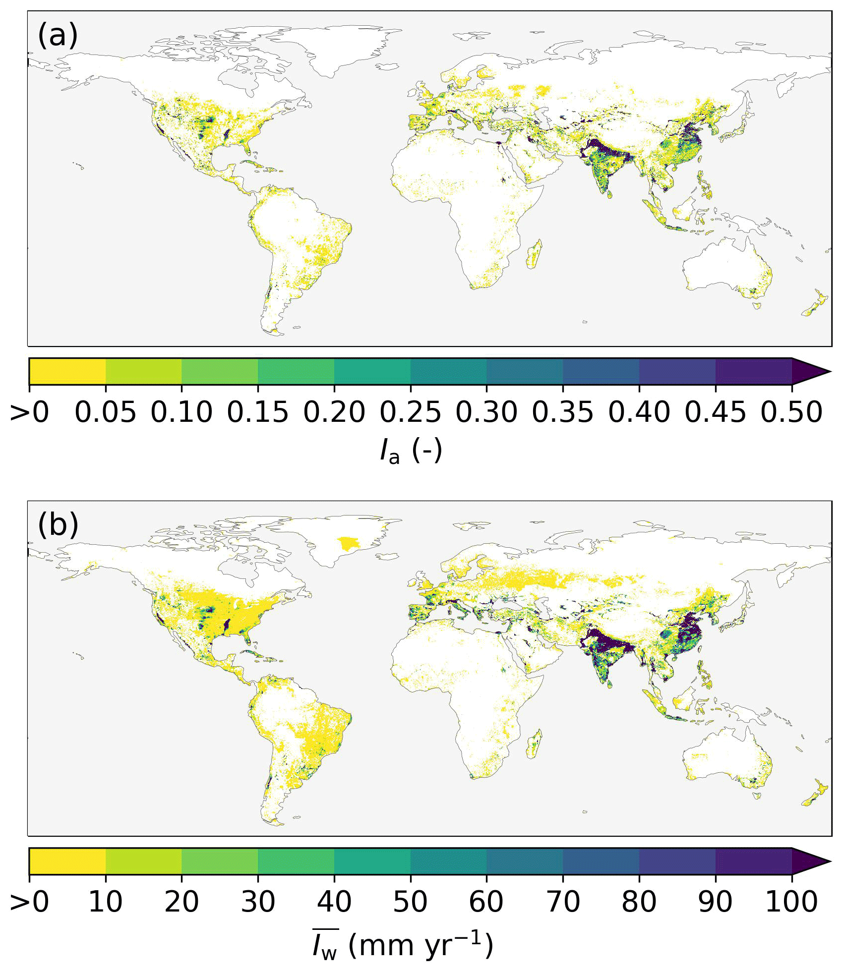
Figure 1Global irrigation characteristics. (a) Irrigated area fraction (Ia, –) representative of 2005 based on subnational irrigation statistics and the HYDE 3.1 land use data (Siebert et al., 2015b). (b) Annual mean irrigation water use (, mm yr−1) for the 2011–2018 period based on multiple satellite-based products and the PT-JPL model (Zhang et al., 2022). White areas indicate Ia or equal to zero.
To identify the effects of irrigation for different regions, we used the Köppen–Geiger climate classes as a climate indicator. For each catchment, we selected the predominant Köppen–Geiger climate class based on a global map at a 1 km resolution representing the 1980–2016 period (Beck et al., 2018a). The gridded data products for P, Ep, Ia, and were converted to catchment estimates using area-weighted averages of the grid cells with more than 50 % of their area located inside the catchment. Before area weighting, the gridded products were resampled to a spatial resolution of 0.05° using nearest-neighbor interpolation. This way, all gridded products were treated similarly and problems with small catchments with no matching grid cells were avoided.
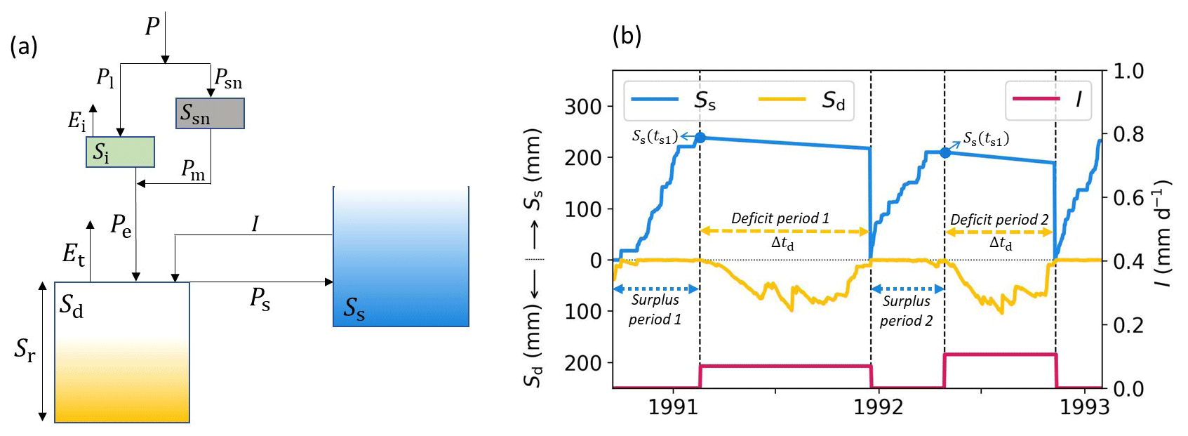
Figure 2(a) Schematic bucket model representation of the memory method including an irrigation model showing storages (mm) – interception storage (Si), snow storage (Ssn), storage deficit (Sd), surplus storage (Ss), and root zone storage capacity (Sr) – and fluxes (mm d−1) – total precipitation (P), liquid precipitation (Pl), precipitation falling as snow (Psn), interception evaporation (Ei), snowmelt (Pm), effective precipitation (Pe), transpiration (Et), precipitation surplus (Ps), and irrigation (I). (b) An example time series of Ss, Sd, and I based on Eqs. (1–6), where Δtd is the length of the deficit period (days) and Ss(ts1) is the surplus storage at the end of the surplus period. Note that this time series represents only 2 years to illustrate the method, while all catchments have at least 10 years of data.
2.2 Memory method with irrigation methods
Figure 2a shows a conceptualization of the memory method based on four storage components (mm): interception storage (Si), snow storage (Ssn), “surplus” storage (Ss), and storage deficit (Sd). Sd is initially conceptualized as an infinite deficit storage volume and its temporal evolution can be described by
where Pe represents effective precipitation (mm d−1), Et is transpiration (mm d−1), I is irrigation (mm d−1), and Ps is surplus precipitation (mm d−1) (Fig. 2a). In Eq. (1), t0 corresponds to the first day of the first hydrological year and τ corresponds to the daily time steps ending on the last day of the last hydrological year. Our hydrological year starts the first day of the month after the wettest month, which is defined as the month with the largest positive difference between monthly mean P and Ep on average. At t0, the starting point of the analysis, Sd=0. In Eq. (1), Pe (mm d−1) is calculated from the water balance of the interception storage Si (Fig. 2a), and Et (mm d−1) is described as a fraction of daily potential evaporation Ep (mm d−1) based on the catchment water balance. We used a simple snow model based on the degree-day method (e.g., Bergstrom, 1975; Gao et al., 2017) to account for the delay in liquid water input to the soil by describing liquid precipitation (Pl, mm d−1), precipitation falling as snow (Psn, mm d−1), and snowmelt (Pm, mm d−1). The equations for the interception storage, snow storage, and transpiration calculation are described in Appendix A.
Surplus precipitation Ps (mm d−1) in Eq. (1) is described by Eq. (2), in which we used the following notation for the sum of the fluxes between two time steps: , where F is either Pe, Et, I, or Ps. Thus Ps,t is described by
with Sd and It approaching zero during periods of abundant precipitation. Hence, it then holds that .
For the computation of applied irrigation (I), we split the time series into surplus and deficit periods (Fig. 2b). For each hydrological year, we defined one deficit period, which is the longest deficit period with the largest Sd in the hydrological year. Surplus periods were defined as the periods in between the deficit periods. For each surplus period, the surplus precipitation Ps (Eq. 2) accumulates in the surplus store Ss:
where ts0 is the first day of the surplus period and ts1 is the last day of the surplus period (Fig. 2b). Ss does not have a maximum storage capacity, but it is reset to zero each year, after each deficit period. This storage conceptualizes any water buffers that can be used for irrigation in the consecutive deficit period and may encompass ditches, lakes, and aquifers. This method assumes that irrigated water only originates from water inside the catchment boundaries and that it is sustainably extracted so that the long-term water balance is closed. During a deficit period, the fraction of Ss that is used for irrigation is defined by irrigation factor f (–), which determines how much of the surplus water stored during the surplus period is used for irrigation during the consecutive deficit period. f represents both the water evaporated or discharged during the irrigation process before recharging the soil and the spatial extent of the irrigation. It is assumed that daily irrigation I is equally distributed over the deficit period (Fig. 2b), so that I (mm d−1) is defined as follows:
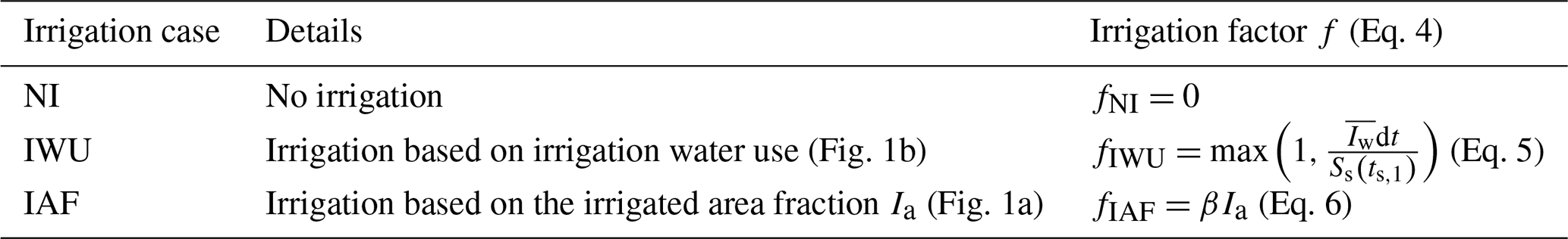
where Δtd is the length of the deficit period (td1−td0) in days (Fig. 2b). Here, based on the two irrigation data sources used (Sect. 2.1), we have developed two methods to estimate f in Eq. (4):
-
The first of these techniques is the “irrigation water use” method (IWU), in which fd,IWU (–) is defined for each deficit period d for each catchment by
Here, (mm yr−1) is the catchment annual mean irrigation water use, dt=1 yr, and Ss(ts,1) (mm) is the surplus storage at the end of the surplus storage accumulation period, i.e., the amount of water stored in Ss at the start of the deficit period. In this method, fd,IWU is different for each deficit period d, as Ss also varies. For each catchment, fIWU is defined as the average fd,IWU.
-
The second of these techniques it the “irrigated area fraction” method (IAF), in which fIAF (–) is temporally non-varying and is defined for each catchment by
where Ia (–) is the catchment irrigated area fraction and β (–) is a correction factor that is constant in space and time for all catchments. β was chosen as a constant to create a relatively simple approach that does not directly rely on irrigation water use data, which is beneficial for application in time periods (both historical and future) without irrigation water use data as well as in regions where no reliable irrigation water use data are available. We estimated β by minimizing the difference between fIAF and fIWU in terms of the root-mean-square error (RMSE). We generated 1000 linearly spaced values for β between 0 and 2.5 and computed fIAF for all the catchments. For all of these cases, the RMSE of catchment fIAF and fIWU was computed (Fig. 3). The RMSE was lowest for β=0.9 (RMSE=0.042), which is applied for all catchments in Eq. (6).
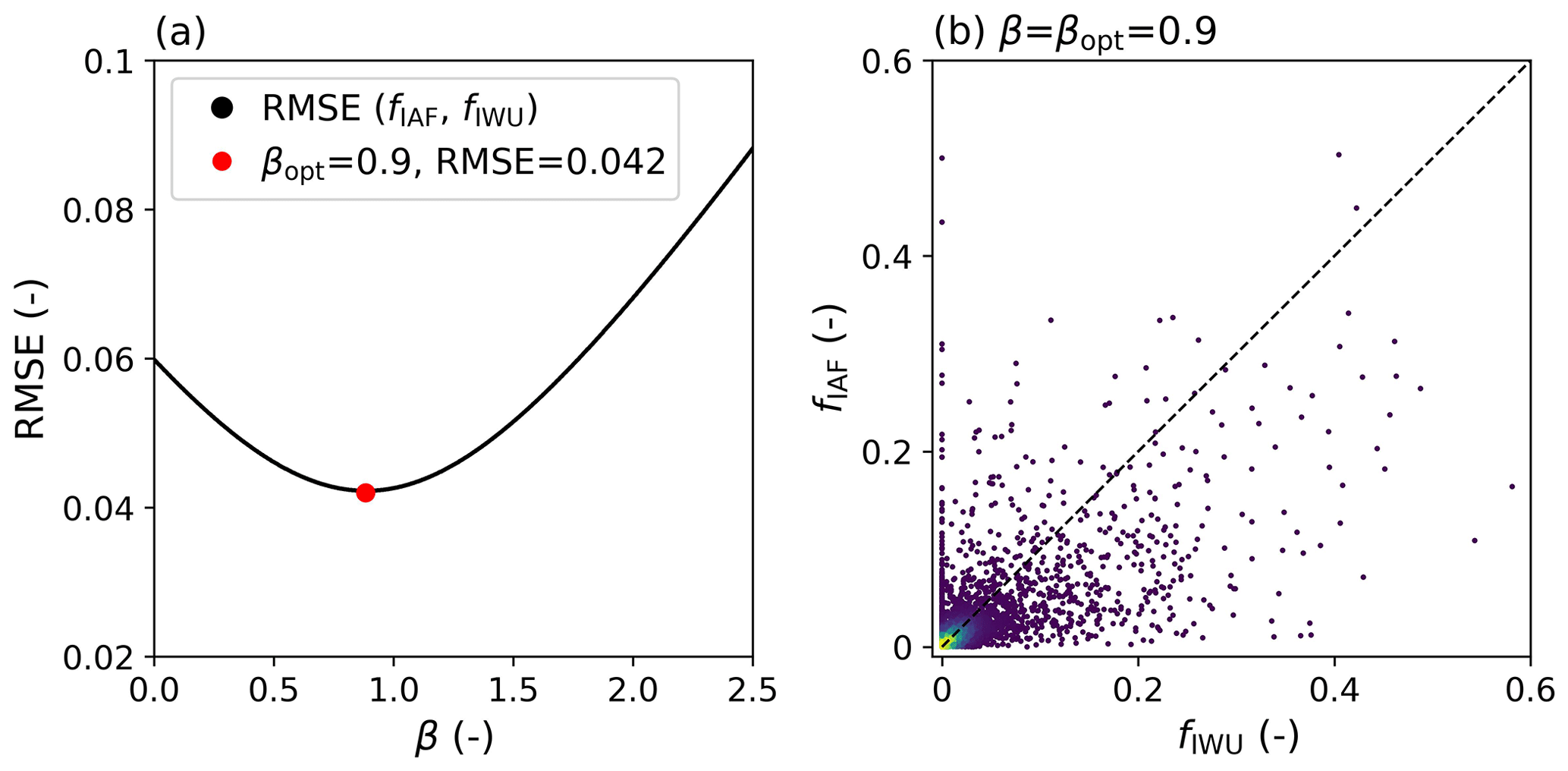
Figure 3The root-mean-square error (RMSE) between the catchment irrigation factors fIWU (Eq. 5) and fIAF (Eq. 6) for 4856 catchments for 1000 linearly spaced values of β between 0 and 2.5. βopt represents the value for β where the RMSE minimizes. (b) Scatterplot of fIWU (Eq. 5) and fIAF (Eq. 6) for β=βopt=0.9, with lighter colors indicating a higher point density.
To evaluate the effect of these methods on estimated Sr, we tested a third case, referred to as “no irrigation” (NI), in which fNI=0. A priori, we cannot and do not consider either of the two methods, i.e., the IWU or the IAF method, to be more representative than the other. While the IWU method uses the irrigation data more directly than the IAF method, the latter directly takes the interannual variability in surplus water into account.
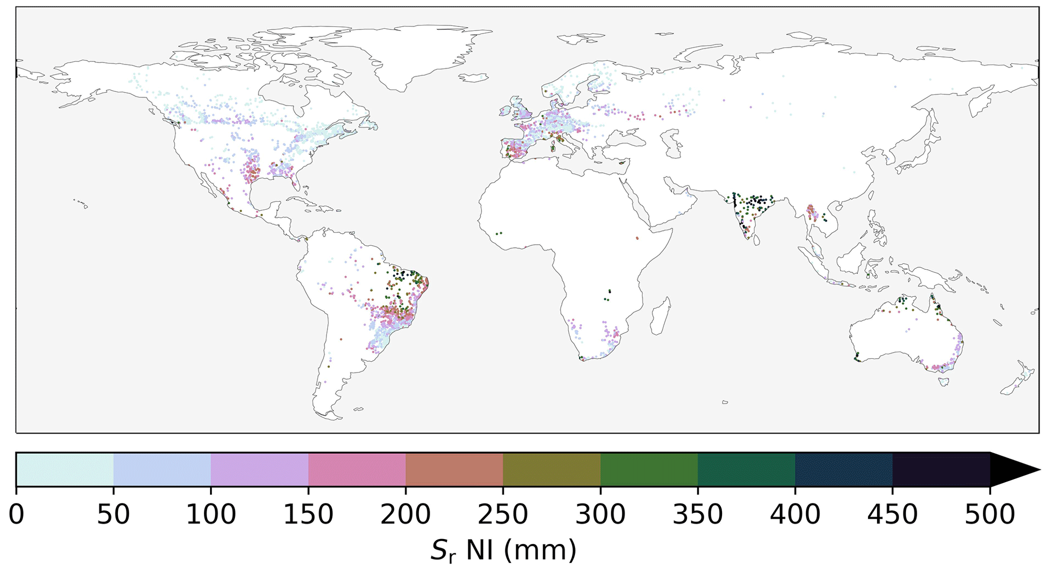
Figure 4Catchment Sr for the no irrigation (NI) case, with dots representing catchment outlets. Similar panels for the IWU and IAF cases are presented in Fig. S3.
2.2.1 Root zone storage capacity calculation
Here, the catchment-scale root zone storage capacity Sr was derived from the catchment-scale storage deficit Sd time series for the three different irrigation cases NI, IWU, and IAF (Table 1). For each catchment, the annual maximum storage deficits (Sd,M) were defined for each hydrological year as follows:
with the min(Sd) occurring earlier in the hydrological year than the max(Sd). Previous studies (e.g., Gao et al., 2014; Wang-Erlandsson et al., 2016) applied a Gumbel distribution to the Sd,M values to estimate Sr for different return periods T. Wang-Erlandsson et al. (2016) found that the best evaporation simulations for croplands, and thus irrigated land, with a global hydrological model were achieved with an Sr based on a return period of 2 years, as croplands adapt to survive droughts with relatively short return periods. Here, we directly used the observed Sd,M values with occurrences closest to T=2 years instead of a fitted extreme value distribution, because fitting an extreme value distribution is ambiguous for return periods of interest (here 2 years) much smaller than the time series length (here >10 years). For all catchments, for each irrigation case separately, the Sr was estimated as the mean of the three observed Sd,M values with occurrences closest to T=2 years, as represented by the cross-markers closest to the vertical dashed line at T=2 years in Fig. 5b, d, f, and h.
Table 1Details of the irrigation cases considered in this study.
2.2.2 Evaluation
To visualize the effects of irrigation on Sd and Sr, we selected four example catchments with different irrigation magnitudes (i.e., Ia and ) located on four different continents and in different climate zones. For quantification of the effects of irrigation on Sr, we computed absolute (Δ) and relative (Δr) differences between the Sr estimates for the NI, IWU, and IAF cases (Table 1). Catchments were stratified based on (1) four different ranges of irrigated area Ia, namely, Ia≤0.01, 0.01, , and Ia>0.1 (Fig. S1 in the Supplement); (2) regions – South America, North America, Europe, and Asia; and (3) climate zones based on the Köppen–Geiger climate classification – subdivided into tropical (Af, Am, and Aw), arid (BWh, BWk, BSh, and BSk), temperate (Cfa, Cfb, and Cfc), Mediterranean (Csa and Csb), and continental (Dfa, Dfb, Dfc, and Dfd) climates (Beck et al., 2018a) (Fig. S2). Uncertainty in the differences in Sr were represented by the interquartile range (IQR).
3.1 Irrigation influence on root zone storage capacity
Globally, the Sr estimates without accounting for irrigation ranged from 0 to 800 mm, with larger values in semiarid regions with high rainfall seasonality, such as northeastern Brazil (median Sr≈250 mm), or monsoon regions, such as northeastern Indian (median Sr≈450 mm), than in regions with temperate climates with year-round rainfall, such as western Europe (median Sr≈70 mm), or continental, colder, climates, such as Canada (median Sr≈40 mm) (Fig. 4).
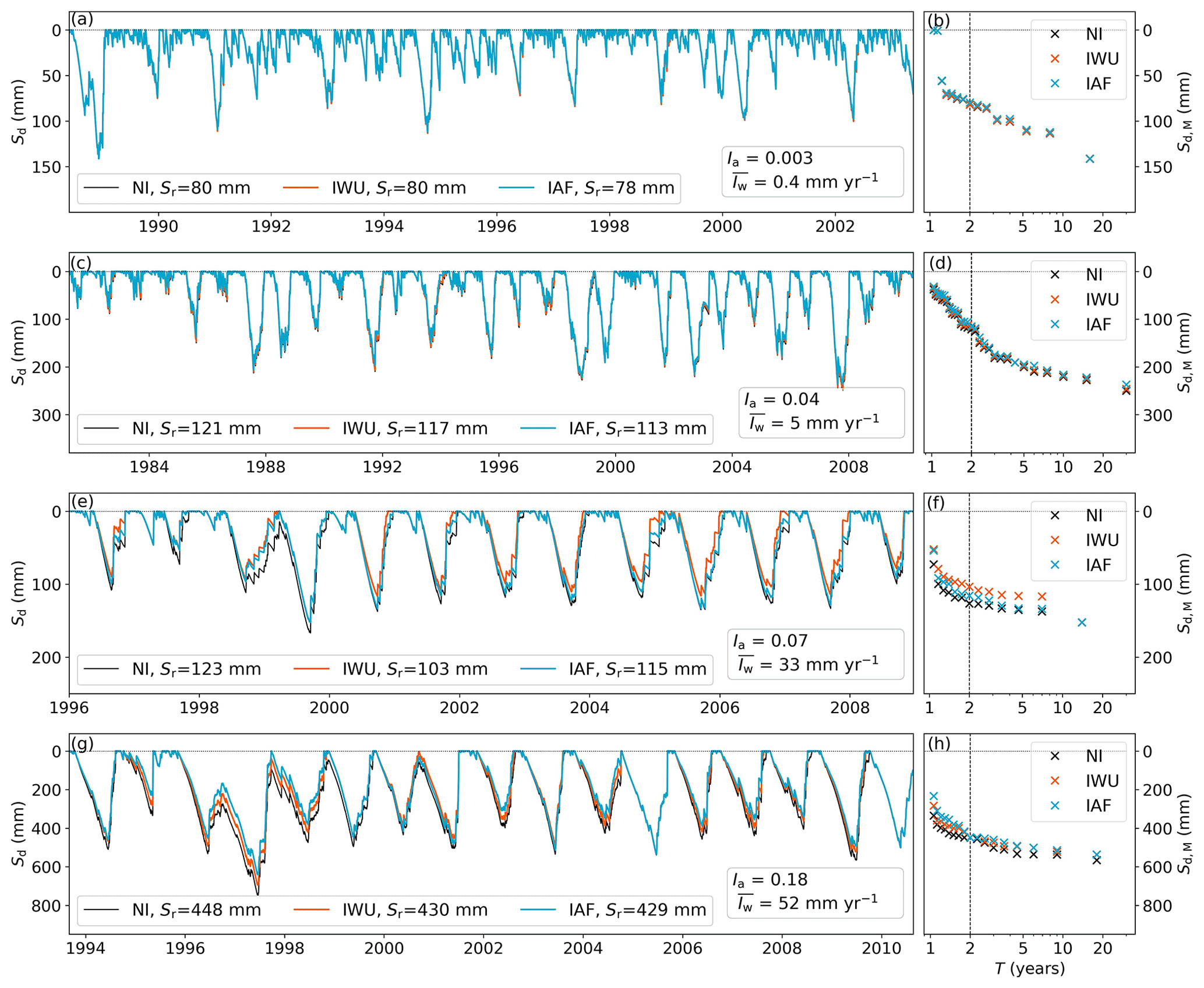
Figure 5(a, c, e, g) Time series of storage deficits Sd (mm) (Eq. 1) for four illustrative catchments with increasing irrigation from top to bottom for the three irrigation cases, NI, IWU, and IAF (Table 1); for each catchment, the associated annual mean irrigation water use (), irrigated area fraction (Ia), and root zone storage capacity (Sr) values are shown. (b, d, f, h) Return-level plot of annual maximum storage deficits (Sd,M) (Eq. 7) for the three irrigation cases (NI, IWU, and IAF), with the vertical dashed line corresponding to a return period (T) of 2 years (Sect. 2.2.1). The locations of the catchments are shown in Fig. 6. The catchment identity, continent, and Köppen–Geiger climate zone are as follows: (a, b) br_0002356, South America, temperate (Cfb); (c, d) ca_0000689, North America, continental (Dfb); (e, f) es_0000742, Europe, Mediterranean (Csa); (g, h) in_0000252, Asia, tropical (Aw).
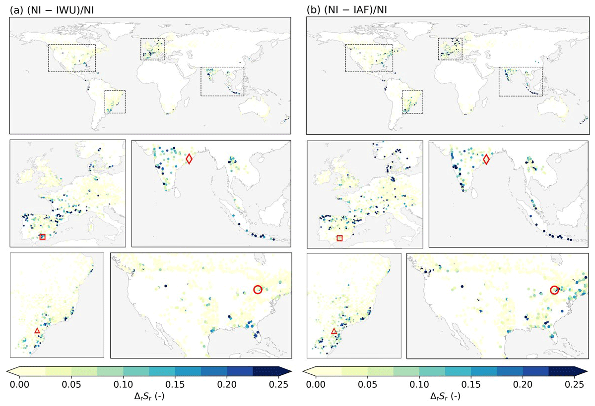
The storage deficits Sd (Eq. 1) generally decreased when accounting for irrigation effects according to the IWU and IAF cases compared with the case without irrigation (NI). These overall effects of the method are illustrated by four selected example catchments in Fig. 5. More pronounced effects of irrigation on Sd are visible for the example catchments in Europe (Fig. 5e and f) and Asia (Fig. 5g and h), with larger and Ia, than in the example catchments in South America (Fig. 5a and b) and North America (Fig. 5c and d). As Sd decreased, the annual maximum storage deficits Sd,M, as determined by Eq. (7), decreased as well. Consequently, the estimated Sr decreased for the IWU and IAF cases compared with NI, with more pronounced effects in the example catchments with larger and Ia (Fig. 5). Globally, Sr consistently decreased for IWU and IAF (Fig. 6), although the magnitudes varied to a considerable extent. Nevertheless, relatively clear regional patterns of the effects of irrigation on Sr emerged. The most pronounced effects cluster in catchments in regions that are characterized by widespread and intense crop cultivation, and thus high irrigation water use, such as northern Spain, France, and parts of India (Fig. 1).
3.2 Regional differences in irrigation influence on root zone storage capacity
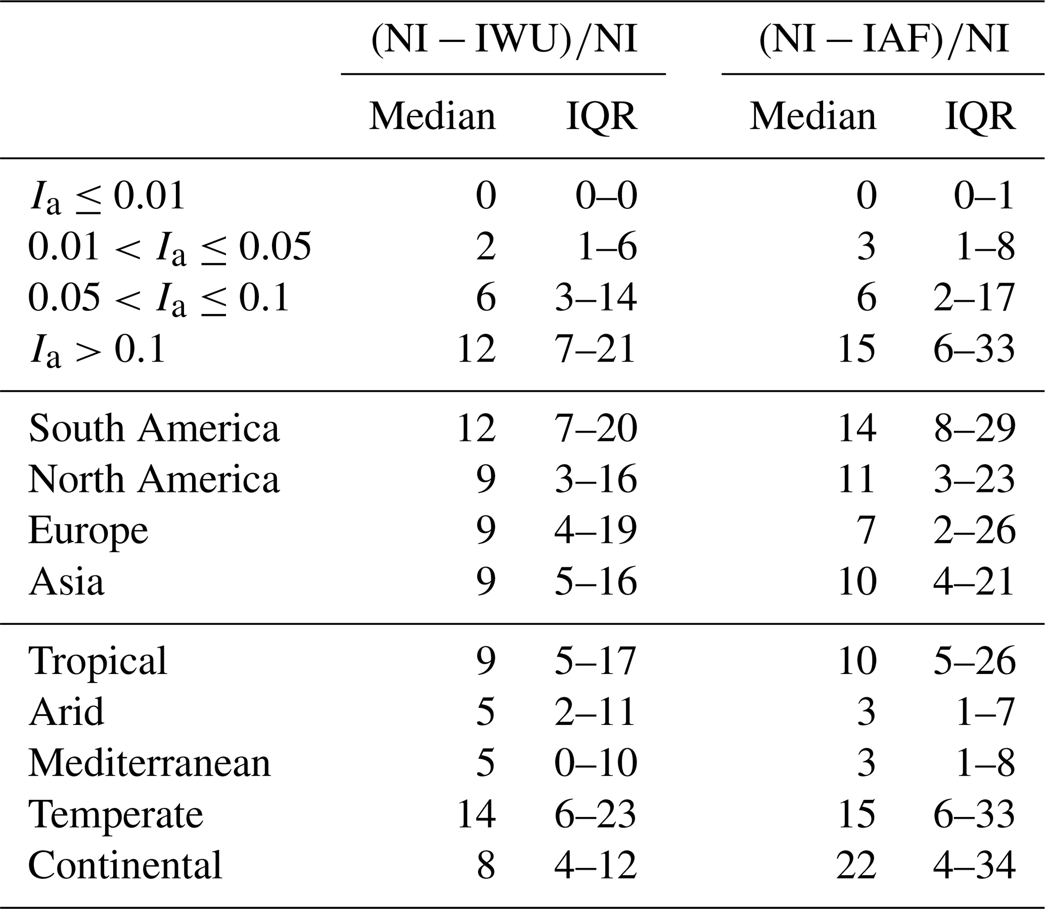
Figure 7 shows that the effects of irrigation on Sr increased with increasing irrigated area fraction Ia for both the IWU and IAF cases. We found the largest effects in catchments with Ia>0.1, such as the example catchment in Asia (Fig. 5g). For these catchments, the median ΔSr was 19 mm (IQR of 10–31 mm) for IWU and 23 mm (IQR of 11–42 mm) for IAF (Fig. 7), corresponding to decreases of 12 % and 15 %, respectively (Table 2). These effects were considerably larger than the effects of irrigation in catchments with , which reached a median ΔrSr of 6 %, corresponding to ΔSr≈9 mm (Fig. 7, Table 2). Although the median effects of irrigation on Sr for catchments with Ia≤0.05 were relatively small, the effects can be considerable for specific individual catchments, as shown by the outliers in Fig. 7.
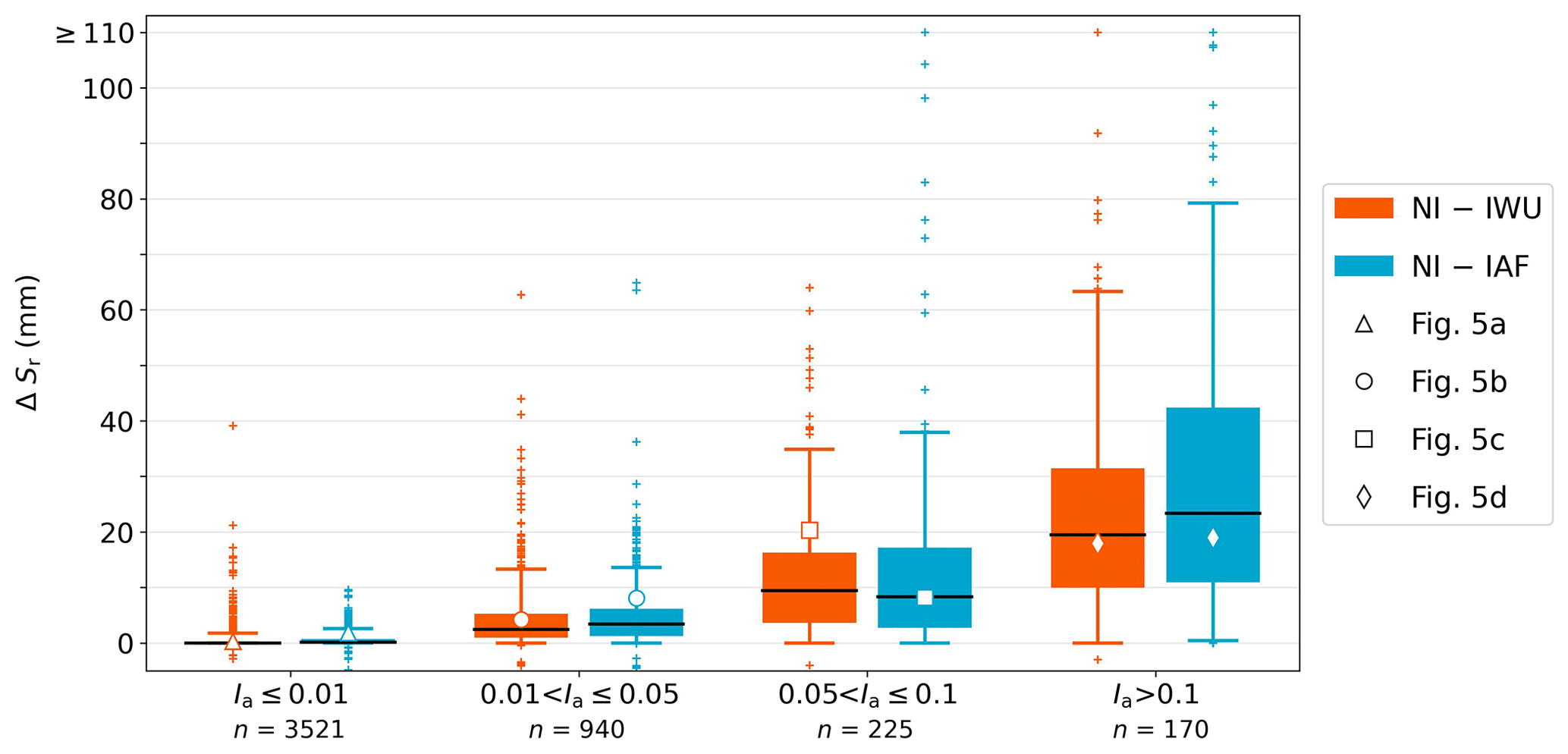
Figure 7Box plots of the absolute Sr difference (ΔSr, m) between the irrigation cases (IWU and IAF) and the no irrigation case (NI) (Table 1). Catchments are stratified in four groups based on the irrigated area fraction Ia (Fig. S2), where n is the number of catchments in each group. The black line represents the median, the box represents the interquartile range (IQR), and the whiskers represent the 5th and 95th percentiles. White markers denote the points presented in Fig. 5. Median and IQR values for relative Sr differences (ΔrSr, %) are presented in Table 2.
The strongest irrigation influence on Sr for catchments with Ia>0.05 was found in Asia, followed by South America, North America, and Europe, for both IWU and IAF (Fig. 8a). For the catchments in Asia, we found median ΔSr values of 21 mm (IQR of 13–41 mm) and 27 mm (IQR of 12–56 mm) for IWU and IAF, respectively . However, the relative differences in Sr (ΔrSr=9 %–10 %) were smaller in Asia than in other regions, reaching up to 14 % in South America, because the initial Sr without accounting for irrigation was considerably larger in Asia than in other regions (Fig. 4, Table 2). Figure 8b shows that Sr decreased the most in tropical catchments, with a median ΔSr of 19 mm for IWU and 24 mm for IAF. These findings are in line with the results presented in Fig. 8a, as most of the tropical catchments that we evaluated were located in Asia (Fig. S3). For catchments in the arid, Mediterranean, temperate, and continental climate zones, the median ΔSr was smaller and varied between 5 and 15 mm. However, catchments in temperate climates exhibited the largest relative influence of irrigation on Sr: median ΔrSr=14 % for IWU and 15 % for IAF (Table 2).
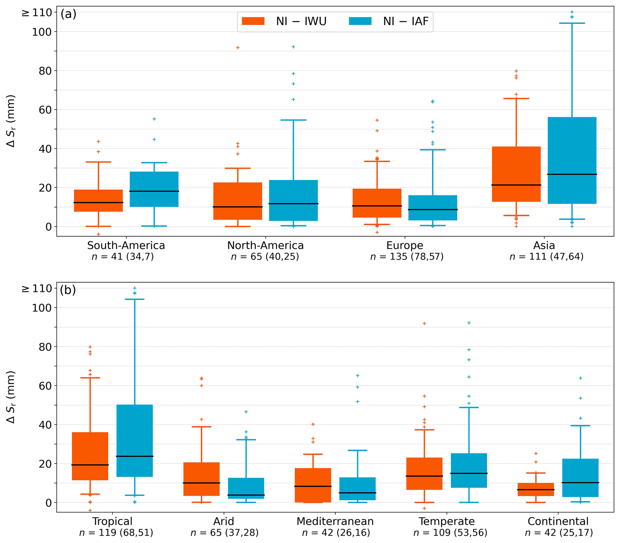
Figure 8Box plots of absolute Sr difference (ΔSr, mm) between the irrigation cases (IWU and IAF) and the no irrigation case (NI) (Table 1). In panel (a) catchments are stratified regionally, similar to the maps in Fig. 6, whereas catchments are stratified based on climate zone (Sect. 2.2.2, Fig. S3) in panel (b); for both panels (a) and (b), only catchments with an irrigated area fraction Ia>0.05 are shown. The total number of catchments (n) in each group is given, with the numbers in parentheses representing n for and Ia>0.1, respectively. The black line represents the median, the box represents the interquartile range (IQR), and the whiskers represent the 5th and 95th percentiles. Median and IQR values for relative Sr differences (ΔrSr, %) are presented in Table 2.
3.3 Comparison of the IWU and IAF methods
Figure 6 shows similar spatial patterns of ΔrSr for IWU and IAF, but the magnitudes differ. For most groups of catchments, IAF had a more pronounced effect on Sr than IWU (Table 2; Fig. S4). The different results for IWU and IAF can be explained by the different methodologies (Table 1). The IWU method directly used annual mean irrigation water use () from Zhang et al. (2022) as an estimate for I (if sufficient water was available in the surplus store Ss). On the other hand, in the IAF method I was defined as a fraction of Ss based on the irrigated area fraction (Ia) and the constant β. Therefore, the estimated I in IAF directly reflected the interannual variability in surplus water. Another cause of the different results for IWU and IAF lies in the estimation of β in IAF, which was based on minimization of the differences between fi,IWU and fi,IAF (Sect. 2.2; Fig. 3). In spite of this optimization, differences between fi,IWU and fi,IAF remained, which partially explain the differences in ΔSr between the two methods.
Table 2Median and interquartile range (IQR) of the relative Sr difference (ΔrSr, %) between the irrigation cases (IWU and IAF) and the no irrigation case (NI) with the catchments stratified based on irrigated area fraction (Ia; Fig. 7) in the top four rows, based on region (only catchments with Ia>0.05; Fig. 8a) in the middle four rows, and based on climate zones (only catchments with Ia>0.05; Fig. 8b) in the bottom five rows. The IQR is given as the 25th percentile–75th percentile.
4.1 Synthesis of results
Our results show that the effect of irrigation on Sr is discernible in all regions, but the magnitude of the effect depends on the amount of irrigation applied (Figs. 5–8). For many parts of the world, the integration of irrigation in the Sr estimation did not have a large influence (Fig. 6). However, Sr considerably decreased for catchments with irrigated area fractions Ia>0.05, and ignoring irrigation in these regions would lead to biased estimates of Sr and, as a consequence, inadequate modeling of vegetation transpiration (Fig. 7). The reduction in Sr in catchments with irrigation was expected based on the fact that the memory method is founded on the theory that vegetation will invest less in roots if sufficient water is available (Guswa, 2008). Here, the observed changes in Sr are attributed to changes in the roots of vegetation, as they are directly related to the size of Sr. Additionally, adaptations at the plant scale associated with irrigation, such as adjustments in stomatal aperture (Chaves et al., 2016) and root hydraulic conductance (Lo Gullo et al., 1998), are also implicitly related to changes in Sr. The influence of irrigation on Sr estimates, as presented in Fig. 6, resembles the spatial pattern found in global assessments of irrigation water withdrawal (Huang et al., 2018) and the extent of irrigation activities (McDermid et al., 2023). This was expected because we used similar underlying irrigation data in the irrigation methods developed here. Given the ongoing irrigation expansion as presented by McDermid et al. (2023), it is expected that larger irrigation water volumes will lead to further reductions in Sr at catchment scales in the near-future compared with the reductions reported in this study. At the same time, irrigation efficiency is also improving (McDermid et al., 2023), but this effect on Sr is less straightforward. Improved irrigation efficiency (i.e., reduced soil evaporation) reduces the irrigation water volumes needed, which, at the catchment scale, leads to increased long-term mean discharge, and thus reduced long-term mean evaporation. This would result in reduced Sr in the memory method compared with a situation with lower irrigation efficiency. However, it has been shown that increased efficiency does not necessarily lead to reduced irrigation water use, as the saved water due to increasing irrigation efficiency is often applied elsewhere (Grafton et al., 2018; Lankford et al., 2020).
Previous studies using the memory method have not considered irrigation in Sr estimates (e.g., De Boer-Euser et al., 2016; Stocker et al., 2023), nor have they evaluated its effects (Wang-Erlandsson et al., 2016). To put our results into perspective, we looked at the effects of snow accumulation and melt on Sr estimates from Dralle et al. (2021) for the continental United States, as this process alters the Sd time series in a similar way to irrigation by temporally shifting liquid water input into the system. Dralle et al. (2021) estimated that integrating snow accumulation and melt in the memory method led to an average reduction in Sr of 6 mm (2 %) for areas with >10 % winter snow coverage and of 28 mm (17 %) for areas with >80 % winter snow coverage (Dralle et al., 2020b). These magnitudes are broadly consistent with our findings for irrigation (Table 2). Our results indicate that the effects of snow and irrigation on Sr are comparable. In our study, 27 catchments have both considerable snowfall (snow days >5 % of the total days) and irrigation (Ia>0.05). For these catchments, the snow model (Appendix A) led to an Sr reduction of 7 mm (7 %) on average for the NI case compared with a setup without the snow model. With irrigation, Sr further decreased by 6 mm (7 %) and 11 mm (12 %) for IAF in these catchments.
Both the results of IWU and IAF showed considerable effects of irrigation on Sr (Figs. 6–8), and both are suitable for use in the memory method, keeping in mind the individual uncertainties related to data and methodological assumptions. We think that the IWU method is more suitable for regional applications for periods with available Iw data (Zhang et al., 2022) than IAF, as Iw was derived from water balances, which strongly depend on the evaluated period. However, for spatial and temporal extrapolation, the direct use of the Iw data in the IWU method is more uncertain than the simpler IAF method, as the irrigated area fraction (Ia) used in IAF is expected to be temporally less variable than the water used for irrigation (Iw). Therefore, we think that the simpler parameterized IAF method is more suitable for use in the memory method for global applications and varying time periods. Moreover, IAF has the potential to be integrated dynamically in hydrological or land surface models employed for global Earth system model studies and future predictions.
4.2 Methodological limitations
By using several data sources, we obtained a large sample of 4856 catchments on different continents, characterized by a wide spectrum of climates and, in particular, regions with various levels of irrigation activity. However, the global coverage is not entirely balanced because Africa and large parts of Asia were undersampled. A further limitation may arise from the assumption in the memory method with irrigation methods proposed here that catchments are hydrologically closed systems. However, inter-catchment lateral flows, such as groundwater and irrigation water, can significantly alter catchment water balances (e.g., Bouaziz et al., 2018; Fan, 2019; Condon et al., 2020). Moreover, the extraction of fossil groundwater for irrigation (Siebert et al., 2010; Grogan et al., 2017; de Graaf et al., 2019) can violate the assumption of closing water balances for the irrigation methods in the memory method developed here. Our methodology, based on a sustainable water use assumption, provides a lower boundary of Sr reduction in irrigated catchments. It is expected that irrigation exceeding sustainable use would lead to larger Sr reductions than reported here, as more water is available to crops than derived from the water balance in this case. Furthermore, the methodology assumes single succession of excess and deficit periods within a year (Fig. 2b), which is not necessarily representative in regions with double-cropping systems or bimodal monsoons (Biradar and Xiao, 2011). Another limitation was the availability and quality of irrigation data (Sect. 2.1, Fig. 1). The annual mean used in IWU was based on the 2011–2018 period, while the catchment time series varied between 1981 and 2010. Similarly, the Ia that we used represented the 2005 irrigated area fraction (Siebert et al., 2015b). The temporal mismatch between catchment hydrological time series and irrigation data may have led to an overestimation of I for the catchment-specific period, as irrigated area and irrigation techniques and efficiency have developed over the evaluated period (McDermid et al., 2023). Although this inconsistency in the temporal data influences the catchment-specific outcomes, we believe that it did not have a major influence on the quantification of the general patterns of the effects of irrigation on Sr, which was the aim of this study.
An additional source of uncertainty in the application of the memory method, as used in this study, relates to the derivation of Sr from the Sd time series (Fig. 5). Given that an ecosystem has developed its Sr such that it functions optimally and can overcome dry periods (e.g., Guswa, 2008), Sr for a specific time period would correspond to the maximum Sd value observed during that same time period (Sr=max(Sd)). However, it is important to note that the memory method represents a simplified approximation of real ecosystem behavior and has inherent limitations. The most important limitation is that our application of the memory method did not account for the feedback between Sd and , which likely led to an overestimation of Sd (Van Oorschot et al., 2021). In this study, we primarily focused on crops that do not exhibit a multiyear root adaptation for survival, as there is no remaining Sr after each year's harvest. However, the catchments used here are not entirely covered by crops in any of the cases; therefore, we used a return period of 2 years for the Sr estimation (following Wang-Erlandsson et al., 2016).
Using a large sample of catchments globally, the presented results support the hypothesis that irrigation considerably reduces the root zone storage capacity (Sr) estimated with the memory method. We found a median Sr reduction of 12 % (IQR of 7 %–21 %) for the IWU method and of 15 % (IQR of 6 %–33 %) for the IAF method for catchments with an irrigated area fraction Ia>10 %. In general, these effects were less pronounced in catchments with a smaller irrigated area, although the Sr for individual catchments could also be considerably influenced by irrigation. Sr decreased the most for catchments in tropical climates, with a median decrease of 19–24 mm (for Ia>5 %). The reductions in Sr found in this study are of the same order of magnitude as the snow effects on Sr estimated by Dralle et al. (2021). Of paramount relevance for regional-to-global hydrological and climate modeling studies, this study demonstrates the relevance of irrigation for adequately estimating Sr. The irrigation water use can be expected to further increase over the next decades; therefore, the related effects on Sr should be represented in the Earth system models that are used for the next climate projections. The methodological approach developed in this study could be profitably used in this respect.
These equations follow Van Oorschot et al. (2021), who based their methods on Gao et al. (2014), De Boer-Euser et al. (2016), Nijzink et al. (2016), and Wang-Erlandsson et al. (2016). Based on temperature, total precipitation (P, mm d−1) was split into liquid precipitation (Pl, mm d−1) and precipitation falling as snow (Psn, mm d−1) (Fig. 2). As temperature varies with altitude, we divided each catchment into elevation zones of 250 m. For each elevation zone (z), the daily temperature (Tz) was calculated as follows:
where Ta (°C) is the catchment average temperature (GSWP3), λ is the lapse rate of 0.0064 °C m−1, and ΔH (m) is the elevation difference between the elevation zone and the mean elevation. For each elevation zone (z), daily Pl and Psn were defined as follows:
The water balance of the snow storage (Ssn; Fig. 2) for each elevation zone (z) was described by
Equation (A4) can be solved by Eqs. (A5) and (A6), in which we used , where F is either Psn or Pm, for the sum of fluxes between two time steps. Thus, the numerical solution using daily time steps can be described as follows:
where Tt is the threshold temperature for snowfall of 0 °C and M is the snowmelt factor of 2 mm d−1 °C−1. Total catchment Pl, Psn, and Pm were calculated as an area-weighted sum of the values for the different elevation zones.
The calculation of effective precipitation Pe (mm d−1) and transpiration (Et) in Eq. (1) is similar to that in Van Oorschot et al. (2021). The water balance of the interception store (Si; Fig. 2a) is described by
where Pl is the liquid precipitation (mm d−1) and Ei is the interception evaporation (mm d−1). Equation (A7) can be solved by Eqs. (A8)–(A10), in which we used , where F is either Pl, Ei, Pe, or Ep (potential evaporation, mm d−1), for the sum of fluxes between two time steps. Thus, the numerical solution using daily time steps can be described as follows:
where Ep is potential evaporation (mm d−1) and Si,max is the maximum interception storage (mm). The size of Si,max has a minor influence on estimates of Sr as shown by, e.g., Hrachowitz et al. (2021) and Bouaziz et al. (2020), and was therefore set to a constant value of 2.5 mm. Daily transpiration (Et) in Eq. (1) was calculated as a fraction of daily Ep by
where is the long-term mean Et derived from the water balance () and is the long-term mean Ep.
GSIM discharge data were obtained from https://doi.org/10.1594/PANGAEA.887477 (Do et al., 2018b) and https://doi.org/10.1594/PANGAEA.887470 (Gudmundsson et al., 2018b), CAMELS-AUS data were sourced from https://doi.org/10.1594/PANGAEA.921850 (Fowler et al., 2020), LamaH-CE data were downloaded from https://doi.org/10.5281/zenodo.7691294 (Kauzlaric et al., 2023), discharge data for Italian catchments were sourced from http://meteoniardo.altervista.org/ (Lendvai, 2020), GSWP3 precipitation and daily mean temperature were obtained from https://doi.org/10.48364/ISIMIP.886955 (Lange and Büchner, 2020), and potential evaporation from GLEAM v3.5a was downloaded from https://www.gleam.eu/#downloads (Martens et al., 2022, 2017; Miralles et al., 2011). The irrigated area fraction was downloaded from https://doi.org/10.13019/M20599 (Siebert et al., 2015a), and irrigation water use was sourced from https://doi.org/10.11888/Hydro.tpdc.271220 (Xin et al., 2021). The global map of the Köppen–Geiger climate classification was obtained from https://doi.org/10.6084/m9.figshare.6396959 (Beck et al., 2018a, b). The scripts underlying this publication are available from https://github.com/fvanoorschot/python_scripts_vanoorschot2024 or https://doi.org/10.5281/zenodo.11026863 (van Oorschot, 2024a). Data underlying this publication are available from https://doi.org/10.5281/zenodo.10869653 (van Oorschot, 2024b).
The supplement related to this article is available online at: https://doi.org/10.5194/hess-28-2313-2024-supplement.
FvO conceptualized the study and carried out the formal analysis with input from RE and MH. FvO prepared the manuscript with contributions from RE, MH, and AA.
At least one of the (co-)authors is a member of the editorial board of Hydrology and Earth System Sciences. The peer-review process was guided by an independent editor, and the authors also have no other competing interests to declare.
Publisher’s note: Copernicus Publications remains neutral with regard to jurisdictional claims made in the text, published maps, institutional affiliations, or any other geographical representation in this paper. While Copernicus Publications makes every effort to include appropriate place names, the final responsibility lies with the authors.
This paper was edited by Elham R. Freund and reviewed by two anonymous referees.
This work was supported by the Netherlands Organization for Scientific Research (NWO), under grant no. OCENW.XS22.2.109, and by the European Union's Horizon 2020 Research and Innovation program, under grant no. 101004156 (CONFESS project).
Alexandratos, N. and Bruinsma, J.: World agriculture towards 2030/2050: the 2012 revision, Food and Agricultural Organization of the United Nation, https://doi.org/10.22004/ag.econ.288998, 2012. a
Bakker, M. R., Jolicoeur, E., Trichet, P., Augusto, L., Plassard, C., Guinberteau, J., and Loustau, D.: Adaptation of fine roots to annual fertilization and irrigation in a 13-year-old Pinus pinaster stand, Tree Physiol., 29, 229–238, https://doi.org/10.1093/treephys/tpn020, 2009. a
Beck, H. E., Zimmermann, N. E., McVicar, T. R., Vergopolan, N., Berg, A., and Wood, E. F.: Present and future Köppen–Geiger climate classification maps at 1-km resolution, figshare [data set], https://doi.org/10.6084/m9.figshare.6396959, 2018a. a, b, c
Beck, H. E., Zimmermann, N. E., McVicar, T. R., Vergopolan, N., Berg, A., and Wood, E. F.: Present and future köppen–geiger climate classification maps at 1-km resolution, Sci. Data, 5, 1–12, https://doi.org/10.1038/sdata.2018.214, 2018b. a
Bergstrom, S.: The development of a snow routine for the HBV-2 model, Nord. Hydrol., 6, 73–92, https://doi.org/10.2166/nh.1975.0006, 1975. a
Biradar, C. M. and Xiao, X.: Quantifying the area and spatial distribution of double- and triple-cropping croplands in India with multi-temporal MODIS imagery in 2005, Int. J. Remote Sens., 32, 367–386, https://doi.org/10.1080/01431160903464179, 2011. a
Bouaziz, L., Weerts, A., Schellekens, J., Sprokkereef, E., Stam, J., Savenije, H., and Hrachowitz, M.: Redressing the balance: Quantifying net intercatchment groundwater flows, Hydrol. Earth Syst. Sci., 22, 6415–6434, https://doi.org/10.5194/hess-22-6415-2018, 2018. a
Bouaziz, L. J., Steele-Dunne, S. C., Schellekens, J., Weerts, A. H., Stam, J., Sprokkereef, E., Winsemius, H. H., Savenije, H. H., and Hrachowitz, M.: Improved Understanding of the Link Between Catchment-Scale Vegetation Accessible Storage and Satellite-Derived Soil Water Index, Water Resour. Res., 56, 1–22, https://doi.org/10.1029/2019WR026365, 2020. a
Bouaziz, L. J. E., Aalbers, E. E., Weerts, A. H., Hegnauer, M., Buiteveld, H., Lammersen, R., Stam, J., Sprokkereef, E., Savenije, H. H. G., and Hrachowitz, M.: Ecosystem adaptation to climate change: the sensitivity of hydrological predictions to time-dynamic model parameters, Hydrol. Earth Syst. Sci., 26, 1295–1318, https://doi.org/10.5194/hess-26-1295-2022, 2022. a
Brunner, I., Herzog, C., Dawes, M. A., Arend, M., and Sperisen, C.: How tree roots respond to drought, Front. Plant Sci., 6, 547, https://doi.org/10.3389/fpls.2015.00547, 2015. a
Chaves, M., Costa, J., Zarrouk, O., Pinheiro, C., Lopes, C., and Pereira, J.: Controlling stomatal aperture in semi-arid regions – The dilemma of saving water or being cool?, Plant Science, 251, 54–64, https://doi.org/10.1016/j.plantsci.2016.06.015, 2016. a
Collins, D. B. and Bras, R. L.: Plant rooting strategies in water-limited ecosystems, Water Resour. Res., 43, 1–10, https://doi.org/10.1029/2006WR005541, 2007. a
Condon, L. E., Markovich, K. H., Kelleher, C. A., McDonnell, J. J., Ferguson, G., and McIntosh, J. C.: Where Is the Bottom of a Watershed?, Water Resour. Res., 56, e2019WR026010, https://doi.org/10.1029/2019WR026010, 2020. a
De Boer-Euser, T., McMillan, H. K., Hrachowitz, M., Winsemius, H. C., and Savenije, H. H.: Influence of soil and climate on root zone storage capacity, Water Resour. Res., 52, 2009–2024, https://doi.org/10.1002/2015WR018115, 2016. a, b, c, d, e
de Boer-Euser, T., Meriö, L.-J., and Marttila, H.: Understanding variability in root zone storage capacity in boreal regions, Hydrol. Earth Syst. Sci., 23, 125–138, https://doi.org/10.5194/hess-23-125-2019, 2019. a
de Graaf, I. E., Gleeson, T., Van Beek, L., Sutanudjaja, E. H., and Bierkens, M. F.: Environmental flow limits to global groundwater pumping, Nature, 574, 90–94, https://doi.org/10.1038/s41586-019-1594-4, 2019. a
DHPC – Delft High Performance Computing Centre: DelftBlue Supercomputer (Phase 1), https://www.tudelft.nl/dhpc/ark:/44463/DelftBluePhase1 (last access: March 2023), 2022. a
Dirmeyer, P., Gao, X., Zhao, M., Guo, Z., Oki, T., and Hanasaki, N.: GSWP-2: Multimodel Analysis and Implications for Our Perception of the Land Surface, B. Am. Meteorol. Soc., 87, 1381–1398, https://doi.org/10.1175/BAMS-87-10-1381, 2006. a
Do, H. X., Gudmundsson, L., Leonard, M., and Westra, S.: The Global Streamflow Indices and Metadata Archive (GSIM) – Part 1: The production of a daily streamflow archive and metadata, Earth Syst. Sci. Data, 10, 765–785, https://doi.org/10.5194/essd-10-765-2018, 2018a. a
Do, H. X., Gudmundsson, L., Leonard, M., and Westra, S.: The Global Streamflow Indices and Metadata Archive – Part 1: Station catalog and Catchment boundary, PANGAEA [data set], https://doi.org/10.1594/PANGAEA.887477, 2018b. a
Dralle, D. N., Hahm, W., Rempe, D. M., Karst, N., Anderegg, L. D., Thompson, S. E., Dawson, T. E., and Dietrich, W. E.: Plants as sensors: Vegetation response to rainfall predicts root-zone water storage capacity in Mediterranean-type climates, Environ. Res. Lett., 15, 104074, https://doi.org/10.1088/1748-9326/abb10b, 2020a. a, b
Dralle, D. N., Hahm, W. J., and Rempe, D. M.: Dataset for “Accounting for snow in the estimation of root-zone water storage capacity from precipitation and evapotranspiration fluxes”, HydroShare [data set], http://www.hydroshare.org/resource/ee45c2f5f13042ca85bcb86bbfc9dd37 (last access: June 2023), 2020b. a
Dralle, D. N., Hahm, W. J., Chadwick, K. D., McCormick, E., and Rempe, D. M.: Technical note: Accounting for snow in the estimation of root zone water storage capacity from precipitation and evapotranspiration fluxes, Hydrol. Earth Syst. Sci., 25, 2862867, https://doi.org/10.5194/hess-25-2861-2021, 2021. a, b, c, d, e
Engels, C., Mollenkopf, M., and Marschner, H.: Effect of drying and rewetting the topsoil on root growth of maize and rape in different soil depths, Z. Pflanzener. Bodenkd., 157, 139–144, https://doi.org/10.1002/jpln.19941570213, 1994. a
Fan, Y.: Are catchments leaky?, WIREs Water, 6, e1386, https://doi.org/10.1002/wat2.1386, 2019. a
Fan, Y., Miguez-Macho, G., Jobbágy, E. G., Jackson, R. B., and Otero-Casal, C.: Hydrologic regulation of plant rooting depth, P. Natl. Acad. Sci. USA, 114, 10572–10577, https://doi.org/10.1073/pnas.1712381114, 2017. a
FAO: World Food and Agriculture – Statistical Yearbook 2022, FAO, https://doi.org/10.4060/cc2211en, 2022. a
Fowler, K., Acharya, S. C., Addor, N., Chou, C., and Peel, M.: CAMELS-AUS v1: Hydrometeorological time series and landscape attributes for 222 catchments in Australia, PANGAEA [data set], https://doi.org/10.1594/PANGAEA.921850, 2020. a
Fowler, K. J., Acharya, S. C., Addor, N., Chou, C., and Peel, M. C.: CAMELS-AUS: Hydrometeorological time series and landscape attributes for 222 catchments in Australia, Earth Syst. Sci. Data, 13, 3847–3867, https://doi.org/10.5194/essd-13-3847-2021, 2021. a
Gao, H., Hrachowitz, M., Schymanski, S. J., Fenicia, F., Sriwongsitanon, N., and Savenije, H.: Climate controls how ecosystems size the root zone storage capacity at catchment scale, Geophys. Res. Lett., 41, 7916–7923, https://doi.org/10.1002/2014GL061668, 2014. a, b, c, d, e, f, g, h
Gao, H., Ding, Y., Zhao, Q., Hrachowitz, M., and Savenije, H. H.: The importance of aspect for modelling the hydrological response in a glacier catchment in Central Asia, Hydrol. Process., 31, 2842–2859, https://doi.org/10.1002/hyp.11224, 2017. a
Gentine, P., D'Odorico, P., Lintner, B. R., Sivandran, G., and Salvucci, G.: Interdependence of climate, soil, and vegetation as constrained by the Budyko curve, Geophys. Res. Lett., 39, 2–7, https://doi.org/10.1029/2012GL053492, 2012. a
Grafton, R. Q., Williams, J., Perry, C. J., Molle, F., Ringler, C., Steduto, P., Udall, B., Wheeler, S. A., Wang, Y., Garrick, D., and Allen, R. G.: The paradox of irrigation efficiency, Science, 361, 748–750, https://doi.org/10.1126/science.aat9314, 2018. a
Grogan, D. S., Wisser, D., Prusevich, A., Lammers, R. B., and Frolking, S.: The use and re-use of unsustainable groundwater for irrigation: a global budget, Environ. Res. Lett., 12, 034017, https://doi.org/10.1088/1748-9326/aa5fb2, 2017. a
Gudmundsson, L., Do, H. X., Leonard, M., and Westra, S.: The Global Streamflow Indices and Metadata Archive (GSIM) – Part 2: Quality control, time-series indices and homogeneity assessment, Earth Syst. Sci. Data, 10, 787–804, https://doi.org/10.5194/essd-10-787-2018, 2018a. a
Gudmundsson, L., Do, H. X., Leonard, M., and Westra, S.: The Global Streamflow Indices and Metadata Archive (GSIM) – Part 2: Time Series Indices and Homogeneity Assessment, PANGAEA [data set], https://doi.org/10.1594/PANGAEA.887470, 2018b. a
Guswa, A. J.: The influence of climate on root depth: A carbon cost-benefit analysis, Water Resour. Res., 44, 1–11, https://doi.org/10.1029/2007WR006384, 2008. a, b, c
Hrachowitz, M., Stockinger, M., Coenders-Gerrits, M., Van Der Ent, R., Bogena, H., Lüke, A., and Stumpp, C.: Reduction of vegetation-accessible water storage capacity after deforestation affects catchment travel time distributions and increases young water fractions in a headwater catchment, Hydrol. Earth Syst. Sci., 25, 4887–4915, https://doi.org/10.5194/hess-25-4887-2021, 2021. a, b, c
Huang, Z., Hejazi, M., Li, X., Tang, Q., Vernon, C., Leng, G., Liu, Y., Döll, P., Eisner, S., Gerten, D., Hanasaki, N., and Wada, Y.: Reconstruction of global gridded monthly sectoral water withdrawals for 1971–2010 and analysis of their spatiotemporal patterns, Hydrol. Earth Syst. Sci., 22, 2117–2133, https://doi.org/10.5194/hess-22-2117-2018, 2018. a
Jägermeyr, J., Gerten, D., Heinke, J., Schaphoff, S., Kummu, M., and Lucht, W.: Water savings potentials of irrigation systems: global simulation of processes and linkages, Hydrol. Earth Syst. Sci., 19, 3073–3091, https://doi.org/10.5194/hess-19-3073-2015, 2015. a
Jha, S. K., Gao, Y., Liu, H., Huang, Z., Wang, G., Liang, Y., and Duan, A.: Root development and water uptake in winter wheat under different irrigation methods and scheduling for North China, Agricurt. Water Manage., 182, 139–150, https://doi.org/10.1016/j.agwat.2016.12.015, 2017. a
Kauzlaric, M., Schürmann, S., Ummel, D., and Zischg, A.: Hourly discharge database HydroCH, Zenodo [data set], https://doi.org/10.5281/zenodo.7691294, 2023. a
Kleidon, A.: Global datasets of rooting zone depth inferred from inverse methods, J. Climate, 17, 2714–2722, https://doi.org/10.1175/1520-0442(2004)017<2714:GDORZD>2.0.CO;2, 2004. a
Kleidon, A. and Heimann, M.: A method of determining rooting depth from a terrestrial biosphere model and its impacts on the global water and carbon cycle, Global Change Biol., 4, 275–286, https://doi.org/10.1046/j.1365-2486.1998.00152.x, 1998. a, b
Klein Goldewijk, K., Beusen, A., van Drecht, G., and de Vos, M.: The HYDE 3.1 spatially explicit database of human-induced global land-use change over the past 12,000 years, Global Ecol. Biogeogr., 20, 73–86, https://doi.org/10.1111/j.1466-8238.2010.00587.x, 2011. a
Klepper, B.: Crop root system response to irrigation, Irrig. Sci., 12, 105–108, https://doi.org/10.1007/BF00192280, 1991. a
Klingler, C., Schulz, K., and Herrnegger, M.: LamaH-CE: LArge-SaMple DAta for Hydrology and Environmental Sciences for Central Europe, Earth Syst. Sci. Data, 13, 4529–4565, https://doi.org/10.5194/essd-13-4529-2021, 2021. a
Kuppel, S., Fan, Y., and Jobbágy, E. G.: Seasonal hydrologic buffer on continents: Patterns, drivers and ecological benefits, Adv. Water Resour., 102, 178–187, https://doi.org/10.1016/j.advwatres.2017.01.004, 2017. a
Lange, S. and Büchner, M.: ISIMIP2a atmospheric climate input data, ISIMIP Repository [data set], https://doi.org/10.48364/ISIMIP.886955, 2020. a
Lankford, B., Closas, A., Dalton, J., López Gunn, E., Hess, T., Knox, J. W., van der Kooij, S., Lautze, J., Molden, D., Orr, S., Pittock, J., Richter, B., Riddell, P. J., Scott, C. A., philippe Venot, J., Vos, J., and Zwarteveen, M.: A scale-based framework to understand the promises, pitfalls and paradoxes of irrigation efficiency to meet major water challenges, Global Environ. Change, 65, 102182, https://doi.org/10.1016/j.gloenvcha.2020.102182, 2020. a
Lendvai, A.: Portale dei dati idrologici italiani, http://meteoniardo.altervista.org/ (last access: August 2023), 2020. a, b
Lo Gullo, M. A., Nardini, A., Salleo, S., and Tyree, M. T.: Changes in root hydraulic conductance (KR) of Olea oleaster seedlings following drought stress and irrigation, New Phytol., 140, 25–31, https://doi.org/10.1046/j.1469-8137.1998.00258.x, 1998. a
Lv, G., Kang, Y., Li, L., and Wan, S.: Effect of irrigation methods on root development and profile soil water uptake in winter wheat, Irrig. Sci., 28, 387–398, https://doi.org/10.1007/s00271-009-0200-1, 2010. a
Maan, C., ten Veldhuis, M.-C., and van de Wiel, B. J. H.: Dynamic root growth in response to depth-varying soil moisture availability: a rhizobox study, Hydrol. Earth Syst. Sci., 27, 2341–2355, https://doi.org/10.5194/hess-27-2341-2023, 2023. a
Martens, B., Miralles, D. G., Lievens, H., Van Der Schalie, R., De Jeu, R. A., Fernández-Prieto, D., Beck, H. E., Dorigo, W. A., and Verhoest, N. E.: GLEAM v3: Satellite-based land evaporation and root-zone soil moisture, Geosci. Model Dev., 10, 1903–1925, https://doi.org/10.5194/gmd-10-1903-2017, 2017. a, b
Martens, B., Miralles, D. G., Lievens, H., van der Schalie, R., de Jeu, R. A. M., Fernández-Prieto, D., Beck, H. E., Dorigo, W. A., and Verhoest, N. E. C.: Global Land Evaporation Amsterdam Model (GLEAM) v3.5a, https://www.gleam.eu/#downloads (last access: November 2022), 2022. a
McCormick, E. L., Dralle, D. N., Hahm, W. J., Tune, A. K., Schmidt, L. M., Chadwick, K. D., and Rempe, D. M.: Widespread woody plant use of water stored in bedrock, Nature, 597, 225–229, https://doi.org/10.1038/s41586-021-03761-3, 2021. a
McDermid, S., Nocco, M., Lawston-Parker, P., Keune, J., Pokhrel, Y., Jain, M., Jägermeyr, J., Brocca, L., Massari, C., Jones, A. D., Vahmani, P., Thiery, W., Yao, Y., Bell, A., Chen, L., Dorigo, W., Hanasaki, N., Jasechko, S., Lo, M.-H., Mahmood, R., Mishra, V., Mueller, N. D., Niyogi, D., Rabin, S. S., Sloat, L., Wada, Y., Zappa, L., Chen, F., Cook, B. I., Kim, H., Lombardozzi, D., Polcher, J., Ryu, D., Santanello, J., Satoh, Y., Seneviratne, S., Singh, D., and Yokohata, T.: Irrigation in the Earth system, Nat. Rev. Earth Environ., 4, 435–453, https://doi.org/10.1038/s43017-023-00438-5, 2023. a, b, c, d, e
Meier, J., Zabel, F., and Mauser, W.: A global approach to estimate irrigated areas – A comparison between different data and statistics, Hydrol. Earth Syst. Sci., 22, 1119–1133, https://doi.org/10.5194/hess-22-1119-2018, 2018. a
Milly, P. C. D.: Climate, soil water storage, and the average annual water balance, Water Resour. Res., 30, 2143–2156, https://doi.org/10.1029/94WR00586, 1994. a
Miralles, D. G., De Jeu, R. A., Gash, J. H., Holmes, T. R., and Dolman, A. J.: Magnitude and variability of land evaporation and its components at the global scale, Hydrol. Earth Syst. Sci., 15, 967–981, https://doi.org/10.5194/hess-15-967-2011, 2011. a, b
Miralles, D. G., Brutsaert, W., Dolman, A. J., and Gash, J. H.: On the Use of the Term “Evapotranspiration”, Water Resour. Res., 56, e2020WR028055, https://doi.org/10.1029/2020WR028055, 2020. a
Nijzink, R., Hutton, C., Pechlivanidis, I., Capell, R., Arheimer, B., Freer, J., Han, D., Wagener, T., McGuire, K., Savenije, H., and Hrachowitz, M.: The evolution of root-zone moisture capacities after deforestation: a step towards hydrological predictions under change?, Hydrol. Earth Syst. Sci., 20, 4775–4799, https://doi.org/10.5194/hess-20-4775-2016, 2016. a, b, c
Roodari, A., Hrachowitz, M., Hassanpour, F., and Yaghoobzadeh, M.: Signatures of human intervention-or not? Downstream intensification of hydrological drought along a large Central Asian river: The individual roles of climate variability and land use change, Hydrol. Earth Syst. Sci., 25, 1943–1967, https://doi.org/10.5194/hess-25-1943-2021, 2021. a
Savenije, H. H.: The importance of interception and why we should delete the term evapotranspiration from our vocabulary, Hydrol. Process., 18, 1507–1511, https://doi.org/10.1002/hyp.5563, 2004. a
Savenije, H. H. and Hrachowitz, M.: HESS Opinions “Catchments as meta-organisms – A new blueprint for hydrological modelling”, Hydrol. Earth Syst. Sci., 21, 1107–1116, https://doi.org/10.5194/hess-21-1107-2017, 2017. a
Schlesinger, W. H. and Jasechko, S.: Transpiration in the global water cycle, Agr. Forest Meteorol., 189–190, 115–117, https://doi.org/10.1016/j.agrformet.2014.01.011, 2014. a
Seneviratne, S. I., Corti, T., Davin, E. L., Hirschi, M., Jaeger, E. B., Lehner, I., Orlowsky, B., and Teuling, A. J.: Investigating soil moisture-climate interactions in a changing climate: A review, Earth-Sci. Rev., 99, 125–161, https://doi.org/10.1016/j.earscirev.2010.02.004, 2010. a
Siebert, S., Burke, J., Faures, J. M., Frenken, K., Hoogeveen, J., Döll, P., and Portmann, F. T.: Groundwater use for irrigation – A global inventory, Hydrol. Earth Syst. Sci., 14, 1863–1880, https://doi.org/10.5194/hess-14-1863-2010, 2010. a
Siebert, S., Kummu, M., Porkka, M., Döll, P., Ramankutty, N., and Scanlon, B. R.: Historical Irrigation Dataset (HID), MyGeoHub [data set], https://doi.org/10.13019/M20599, 2015a. a
Siebert, S., Kummu, M., Porkka, M., Döll, P., Ramankutty, N., and Scanlon, B. R.: A global data set of the extent of irrigated land from 1900 to 2005, Hydrol. Earth Syst. Sci., 19, 1521–1545, https://doi.org/10.5194/hess-19-1521-2015, 2015b. a, b, c, d, e
Singh, C., Wang-Erlandsson, L., Fetzer, I., Rockström, J., and Van Der Ent, R.: Rootzone storage capacity reveals drought coping strategies along rainforest-savanna transitions, Environ. Res. Lett., 15, 124021, https://doi.org/10.1088/1748-9326/abc377, 2020. a, b
Singh, C., van der Ent, R., Wang-Erlandsson, L., and Fetzer, I.: Hydroclimatic adaptation critical to the resilience of tropical forests, Global Change Biol., 28, 2930–2939, https://doi.org/10.1111/gcb.16115, 2022. a
Sivandran, G. and Bras, R. L.: Dynamic root distributions in ecohydrological modeling: A case study at Walnut Gulch Experimental Watershed, Water Resour. Res., 49, 3292–3305, https://doi.org/10.1002/wrcr.20245, 2013. a
Speich, M. J., Lischke, H., and Zappa, M.: Testing an optimality-based model of rooting zone water storage capacity in temperate forests, Hydrol. Earth Syst. Sci., 22, 4097–4124, https://doi.org/10.5194/hess-22-4097-2018, 2018. a
Stocker, B. D., Tumber-Dávila, S. J., Konings, A. G., Anderson, M. C., Hain, C., and Jackson, R. B.: Global patterns of water storage in the rooting zones of vegetation, Nat. Geosci., 16, 250–256, https://doi.org/10.1038/s41561-023-01125-2, 2023. a, b, c, d
van Oorschot, F.: Python scripts Van Oorschot et al. (2024), Zenodo [code], https://doi.org/10.5281/zenodo.11026863, 2024a. a
van Oorschot, F.: Data underlying Van Oorschot et al. (2024), Zenodo [data set], https://doi.org/10.5281/zenodo.10869653, 2024b. a
Van Oorschot, F., Van Der Ent, R. J., Hrachowitz, M., and Alessandri, A.: Climate-controlled root zone parameters show potential to improve water flux simulations by land surface models, Earth Syst. Dynam., 12, 725–743, https://doi.org/10.5194/esd-12-725-2021, 2021. a, b, c, d, e
Wang, J., Du, G., Tian, J., Zhang, Y., Jiang, C., and Zhang, W.: Effect of irrigation methods on root growth, root-shoot ratio and yield components of cotton by regulating the growth redundancy of root and shoot, Agricult. Water Manage., 234, 106120, https://doi.org/10.1016/j.agwat.2020.106120, 2020. a
Wang, K. and Dickinson, R. E.: A review of global terrestrial evapotranspiration: Observation, modeling, climatology, and climatic variability, Rev. Geophys., 50, RG2005, https://doi.org/10.1029/2011RG000373, 2012. a
Wang-Erlandsson, L., Bastiaanssen, W. G., Gao, H., Jägermeyr, J., Senay, G. B., Van Dijk, A. I., Guerschman, J. P., Keys, P. W., Gordon, L. J., and Savenije, H. H.: Global root zone storage capacity from satellite-based evaporation, Hydrol. Earth Syst. Sci., 20, 1459–1481, https://doi.org/10.5194/hess-20-1459-2016, 2016. a, b, c, d, e, f, g
Xin, L., Ling, Z., Kun, Z., Donghai, Z., and Gaofeng, Z.: Satellite-based Global Irrigation Water Use data set (2011–2018), TPDC [data set], https://doi.org/10.11888/Hydro.tpdc.271220, 2021. a
Zhang, B., Hautier, Y., Tan, X., You, C., Cadotte, M. W., Chu, C., Jiang, L., Sui, X., Ren, T., Han, X., and Chen, S.: Species responses to changing precipitation depend on trait plasticity rather than trait means and intraspecific variation, Funct. Ecol., 34, 2622–2633, https://doi.org/10.1111/1365-2435.13675, 2020. a
Zhang, K., Li, X., Zheng, D., Zhang, L., and Zhu, G.: Estimation of Global Irrigation Water Use by the Integration of Multiple Satellite Observations, Water Resour. Res., 58, 1–23, https://doi.org/10.1029/2021WR030031, 2022. a, b, c, d, e
Zhao, J., Xu, Z., and Singh, V. P.: Estimation of root zone storage capacity at the catchment scale using improved Mass Curve Technique, J. Hydrol., 540, 959–972, https://doi.org/10.1016/j.jhydrol.2016.07.013, 2016. a