Towards understanding the influence of seasons on low-groundwater periods based on explainable machine learning

Seasons are known to have a major influence on groundwater recharge and therefore groundwater levels; however, underlying relationships are complex and partly unknown. The goal of this study is to investigate the influence of the seasons on groundwater levels (GWLs), especially during low-water periods. For this purpose, we train artificial neural networks on data from 24 locations spread throughout Germany. We exclusively focus on precipitation and temperature as input data and apply layer-wise relevance propagation to understand the relationships learned by the models to simulate GWLs. We find that the learned relationships are plausible and thus consistent with our understanding of the major physical processes. Our results show that for the investigated locations, the models learn that summer is the key season for periods of low GWLs in fall, with a connection to the preceding winter usually only being subordinate. Specifically, dry summers exhibit a strong influence on low-water periods and generate a water deficit that (preceding) wet winters cannot compensate for. Temperature is thus an important proxy for evapotranspiration in summer and is generally identified as more important than precipitation, albeit only on average. Single precipitation events show by far the largest influences on GWLs, and summer precipitation seems to mainly control the severeness of low-GWL periods in fall, while higher summer temperatures do not systematically cause more severe low-water periods.

1 Introduction

Groundwater is a major source of drinking water globally and is also used for agricultural irrigation, industrial purposes, and supplying terrestrial and aquatic groundwater-dependent ecosystems (Gleeson et al., 2016; Siebert et al., 2010). However, groundwater resources are under increasing pressure due to climate change, intensified land use, and increasing groundwater abstraction (Famiglietti, 2014; Green et al., 2011). Low-water periods are thereby of particular interest since they often cause problems, such as for groundwater-dependent ecosystems or water supply. Moreover, they mostly coincide in terms of time with periods of higher water demand and therefore with increased abstraction rates, which exacerbates the problem. The sustainable availability of groundwater resources is chiefly determined by groundwater recharge. Overexploitation occurs when abstraction exceeds recharge. Recharge is difficult to quantify directly and precisely over large areas, but in shallow, unconfined, and unused aquifers, groundwater levels (GWLs) are a good, although not fully quantitative, indicator of recharge. Quantitative calculation of recharge based on groundwater levels would require detailed knowledge of soil water dynamics, effective storage porosity, and hydraulic gradients controlling groundwater flow. Similarly, changes in groundwater levels provide a straightforward way to identify and estimate changes in groundwater availability, with the limitations mentioned above (Hartmann et al., 2012). On longer timescales, recharge is the difference between precipitation and actual evapotranspiration (minus overland flow, if present), including transpiration from groundwater, which can be relevant in shallow aquifers; on shorter timescales, the previous saturation state of the soil (i.e., the soil water deficit) and changes in soil moisture storage play a major role in recharge and, consequently, groundwater levels. During the vegetation period, most of the precipitation is used by the vegetation for evapotranspiration. After long dry periods, large quantities of rainfall are needed to replenish the soil water deficit before recharge can start (Döll and Fiedler, 2008). However, in the cold season, when soils are typically water saturated, most of the precipitation water is available for recharge unless it is stored in the snow cover (Petitta et al., 2022).

These generalized relations show that the seasons have a major impact on groundwater recharge, although the underlying processes and relationships are quite complex and still not completely understood. From glaciology, it is known that the summer season often has a larger impact on glacier retreat than the winter season (Fujita and Ageta, 2000; Thibert et al., 2013; Trachsel and Nesje, 2015). To put it simply, a long, hot, and dry summer can cause more damage to a glacier than a long winter with plenty of snow can repair. Similar relationships have been observed in soil science, where long-term lysimeter data have shown that the negative impact of hot, dry summers on soil water storage is much greater than the positive influence of a wet winter season (Merk et al., 2021). The principal goal of this study is to investigate the influence of the seasons on groundwater levels, especially during low-water periods, and our initial hypothesis is that hot, dry summers have a stronger negative impact on groundwater resources than can be compensated for by (preceding) wet winters.

Data-driven groundwater modeling based on machine learning (ML) methods is now an established yet still emerging field, as shown in a recent review by Tao et al. (2022). The ability of ML models to simulate GWLs based on historic groundwater and meteorological data alone, without comprehensive knowledge and data of the underground structure, makes them appealing compared to physically based and numerical methods (Adamowski and Chan, 2011), and it was found that artificial intelligence (AI) methods (including ML) can successfully be used to simulate and predict GWL time series in different aquifers (Rajaee et al., 2019). Despite their success in terms of good model performance, one often-mentioned drawback of AI and ML models is their “black-box” characteristic as they do not rely on known physical relationships. However, explainable AI (XAI) methods can help to overcome this problem. They allow us to interpret model behavior and thus not only let us build trust in the models but also potentially help us obtain new insights that are not apparent from the data alone. A good overview of XAI methods, including their history, motivation, goals, and types, is given by Samek et al. (2019) and Holzinger et al. (2022). Popular types range from surrogate functions (e.g., local interpretable model-agnostic explanations (LIME); Ribeiro et al., 2016) and local perturbation-based (sensitivity) methods (e.g., SHapley Additive exPlanations (SHAP); Lundberg and Lee, 2017) to propagation-based approaches, which integrate the internal structure of the model into the explanation process. Layer-wise relevance propagation (LRP) (Bach et al., 2015; Montavon et al., 2019) is a propagation-based explanation framework which is applicable to artificial neural networks (ANNs). It decomposes the output of the nonlinear decision function in terms of the input variables, forming a vector of input feature scores that constitute the “explanation” (Lapuschkin et al., 2019). LRP has been extensively applied and validated across numerous disciplines, including computer vision, medicine, natural language processing, and economy. However, to the best of our knowledge, its application in Earth science is limited to Toms et al. (2020) and Mirzavand Borujeni et al. (2023), who use it in the context of the El Niño–Southern Oscillation and surface sea temperature forecasts and with regard to air pollution, respectively. We chose this method since it is rather straightforward, easy to understand and interpret, and applicable to sequence-like/time series input data with deep learning models. Moreover, it has some advantages compared to other XAI methods, such as its high computational efficiency and its theoretical underpinning based on deep Taylor decomposition (Montavon et al., 2017), making it a trustworthy and robust explanation method (Arras et al., 2022).

This study aims to explore different research questions:

1. Is it possible to use LRP to explore what ANNs learn when simulating GWLs with meteorological input data and disentangle the temporal component of such learned relationships?

2. Do these relationships align with our existing conceptual understanding of the relevant processes?

3. What do the models identify as key drivers for low-GWL periods?

4. What is the specific influence of each season and the temporal patterns of precipitation and temperature during these seasons?

To answer these questions, we train one-dimensional (1D) convolutional neural networks (CNNs) at 24 example locations spread throughout Germany and apply LRP to explore what these models learn when they receive meteorological input data to simulate groundwater levels over time. In terms of model choice, we prefer CNNs over recurrent alternatives, such as long short-term memory (LSTM) networks (Hochreiter and Schmidhuber, 1997), because they have been proven to be well suited and reliable in earlier studies (e.g., Wunsch et al., 2022). With regard to input forcing data, we exclusively use precipitation and temperature, which yield good simulation results and, due to the low number of variables, simplify the later interpretation of the learned relationships.

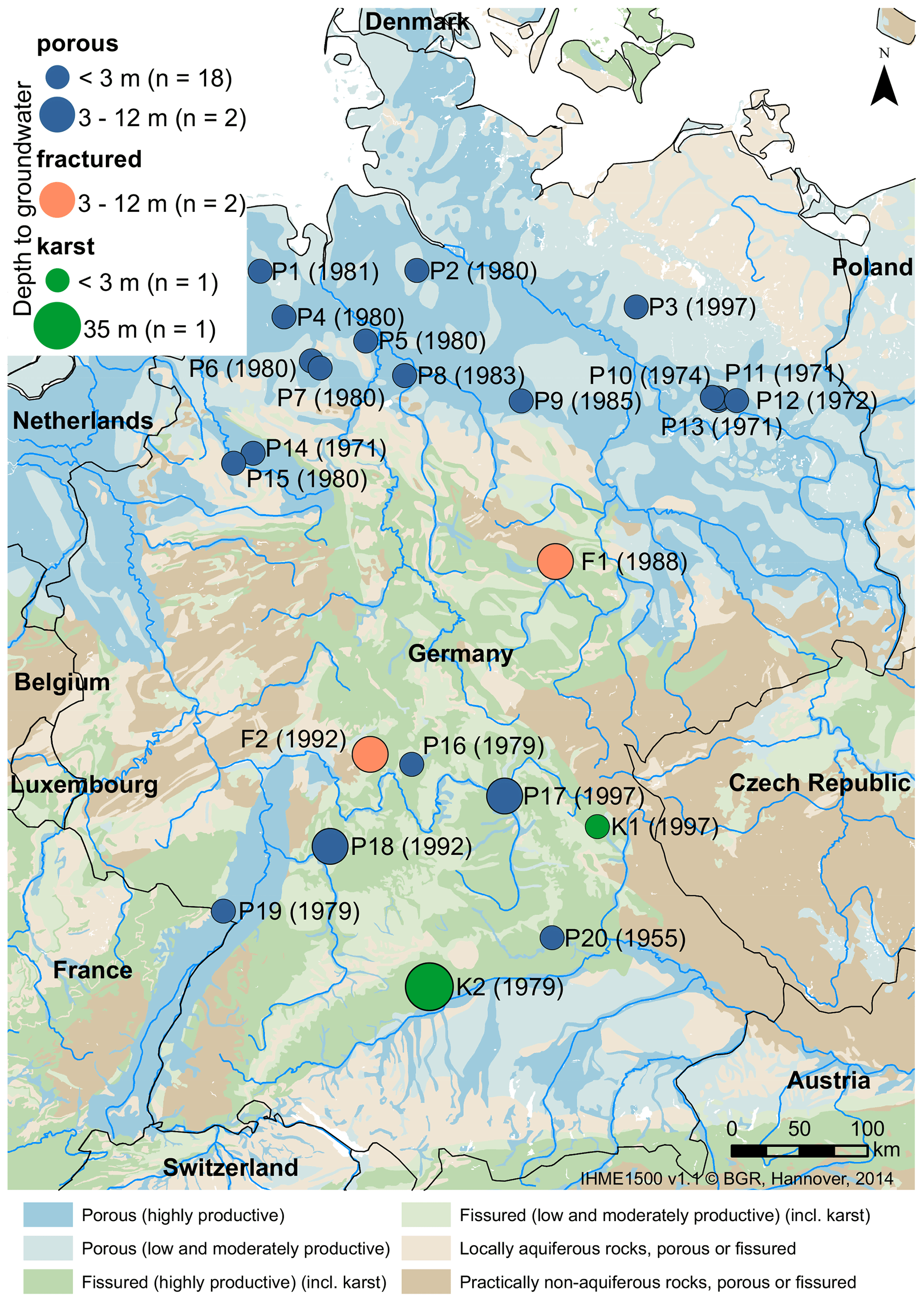
Figure 1 Map of the considered locations in Germany, with each circular symbol indicating the aquifer type of each well (symbol color), the depth to groundwater (symbol size), and an ID specifying the start year of the data records in parentheses (symbol label). The background shows the aquifer type based on the IMHE.

2 Data and methods

2.1 Data and locations

In this study, we use groundwater data from 24 different locations throughout Germany. All locations represent the uppermost, unconfined aquifer and exhibit weekly groundwater time series with a minimum length of 24 years (1997–2020) and a maximum length of 66 years (1955–2020). Most wells are located in very shallow, porous aquifers; however, two wells are located in fractured aquifers and two wells in karst aquifers, with a slightly larger depth to groundwater. The locations, the start year of the weekly data records, the aquifer type, and the depth to groundwater are depicted in Fig. 1. The groundwater data until 2015 are a subset of publicly available data (Wunsch et al., 2021b) and were preprocessed as described in Wunsch et al. (2022). More recent data were added using openly available and gapless groundwater data from the respective online services of the federal environmental agencies.

The input data are precipitation and temperature from the respective locations within the HYRAS (Hydrometeorologische Rasterdatensätze) v5.0 dataset from the German Meteorological Service (Rauthe et al., 2013; Razafimaharo et al., 2020). The HYRAS v5.0 dataset is a downscaled raster dataset with a cell size of 1 km² and is based on observations from meteorological stations; it is openly available via the German Meteorological Service (DWD) (2022). Conceptually, precipitation serves as a proxy for potential groundwater recharge after compensating for deficits in soil water, while temperature represents evapotranspiration processes. Usually, higher temperature also means higher evapotranspiration and thus less potential groundwater recharge; however, the relationships are complex and partly dependent. For example, in winter, higher temperature often goes along with higher precipitation intensity, thus higher potential recharge, because very cold conditions (≪0 °C) are usually dry, whereas in summer, precipitation intensity decreases with increasing temperatures (e.g., Berg et al., 2009).

2.2 Model selection and evaluation

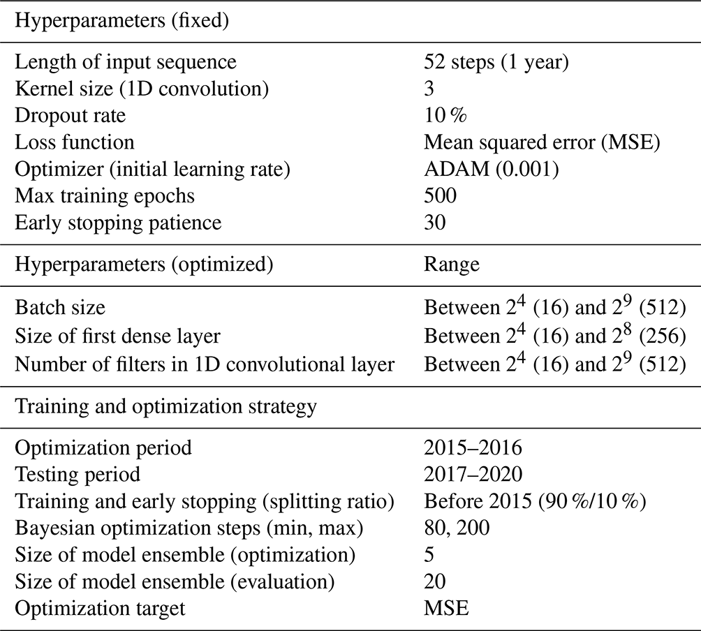
To perform this study, we use convolutional neural networks (CNNs) (LeCun et al., 2015), which are commonly applied to image-like data but have also shown to be valuable for the simulation of sequential data, such as water-related time series (Duan et al., 2020; Wunsch et al., 2021a, 2022). The CNNs applied in this study comprise the layers shown in Fig. 2 and use the hyperparameters listed in Table 1. All models are applied in a sequence-to-value forecasting mode and use a fixed input sequence length of 52 weeks (1 year), as illustrated in Fig. 2. This is necessary to answer the research questions of this study and to enable comparability between models. Bayesian optimization (Nogueira, 2014) is applied to select the optimal configuration for the training batch size, the number of filters in the 1D convolutional layer, and the number of neurons in the first dense layer (according to the range listed in Table 1). Between 80 and 200 optimization steps are performed; above 80, the process stops if no improvement occurs for 25 steps. Because the models depend on a random initialization, we use a model ensemble of 20 independently trained CNNs (with only 5 for each optimization step to save computation time). We derive a 90 % prediction interval from the model ensemble based on these 20 model initializations, meaning that 18 out of 20 model runs fall within the shown interval. All models are implemented in Python 3.8 using TensorFlow 2.7 (Abadi et al., 2015); Keras (Chollet, 2015); and the libraries “NumPy” (van der Walt et al., 2011), “pandas” (The pandas development team, 2024), “scikit-learn” (Pedregosa et al., 2011), and “Matplotlib” (Hunter, 2007).

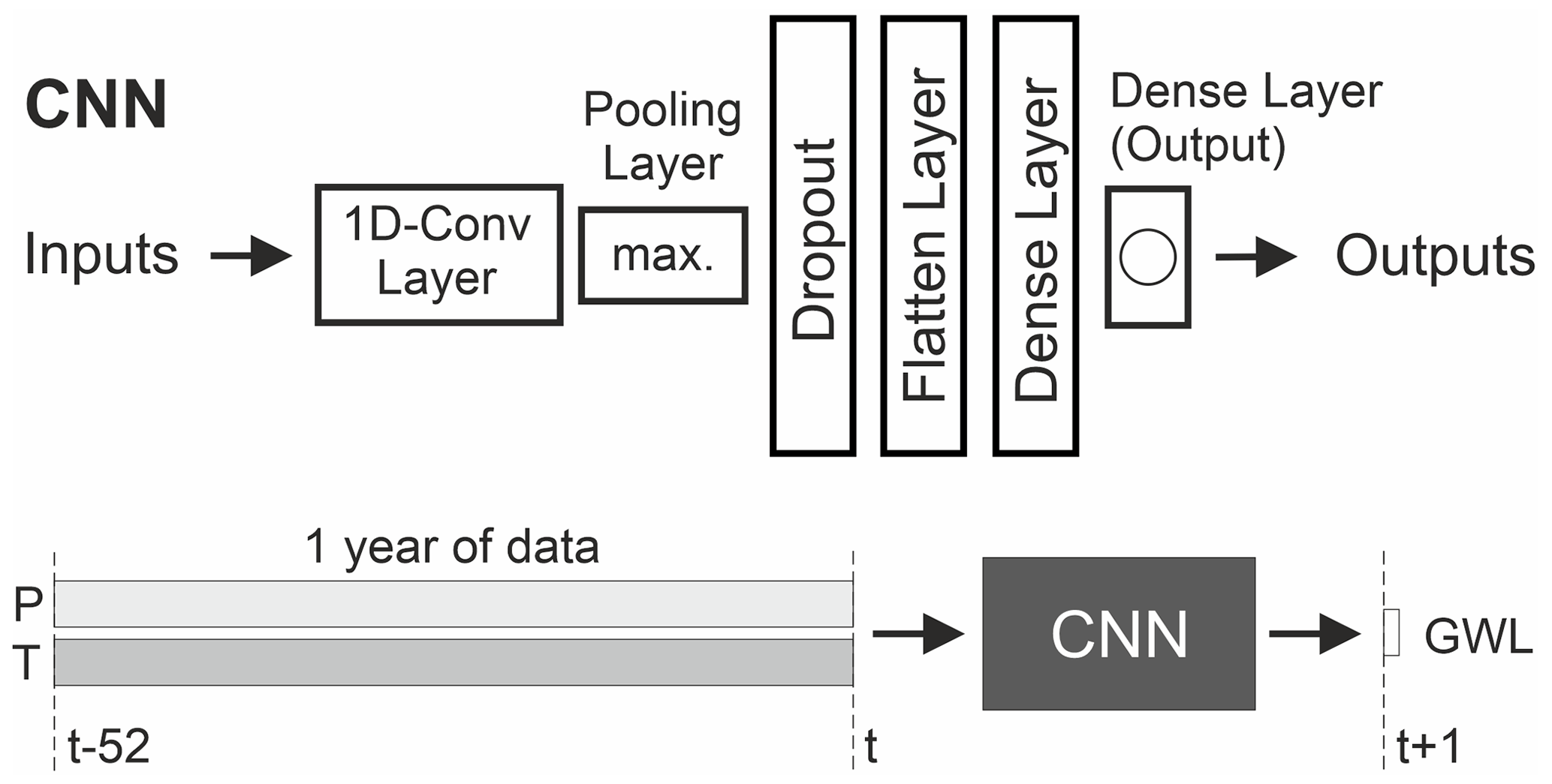
Figure 2 Structure of the CNN models (upper part) and illustration of the sequence-to-value forecasting mode with a fixed input sequence of 1 year (lower part).

Table 1 Summary of the model hyperparameters and important parts of the modeling and evaluation strategy.

We selected only those locations where the tested models achieve particularly good scores in the test set (Fig. 3b; details on each location in the Supplement). This way, we reduce uncertainty from model inaccuracies during the following analyses. However, because we will analyze the model not only in the test period but also in selected periods of the complete individual time series, we explored the model fit for the full time series and selected only locations with a highly accurate fit throughout the complete simulation (Fig. 3a). The simulation accuracy is demonstrated in Fig. 3 using the Nash–Sutcliffe efficiency (NSE) (Nash and Sutcliffe, 1970), coefficient of determination (R²), and Kling–Gupta efficiency (KGE) (Gupta et al., 2009). We also rigorously assessed the fit between observed and simulated values visually across all parts to reduce the possible influence of counterbalancing error effects. An example simulation and an illustration of the time series partition for training, optimization, and testing are depicted in Fig. 4 for location P11.

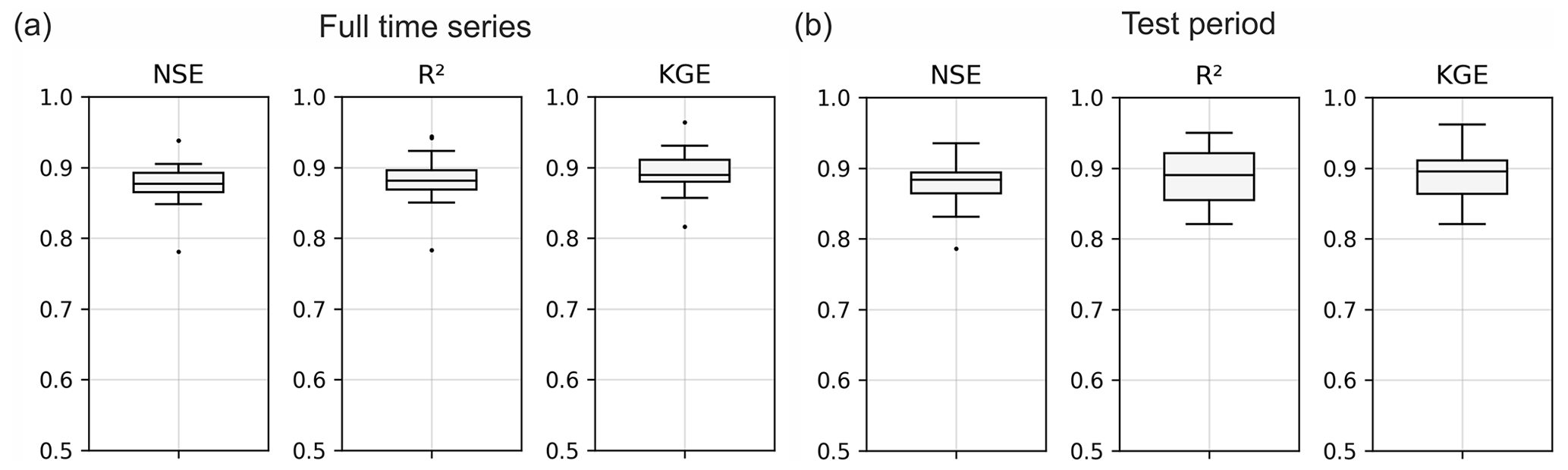
Figure 3 Model performance at all 24 locations for (a) the complete time series and (b) the test period only.

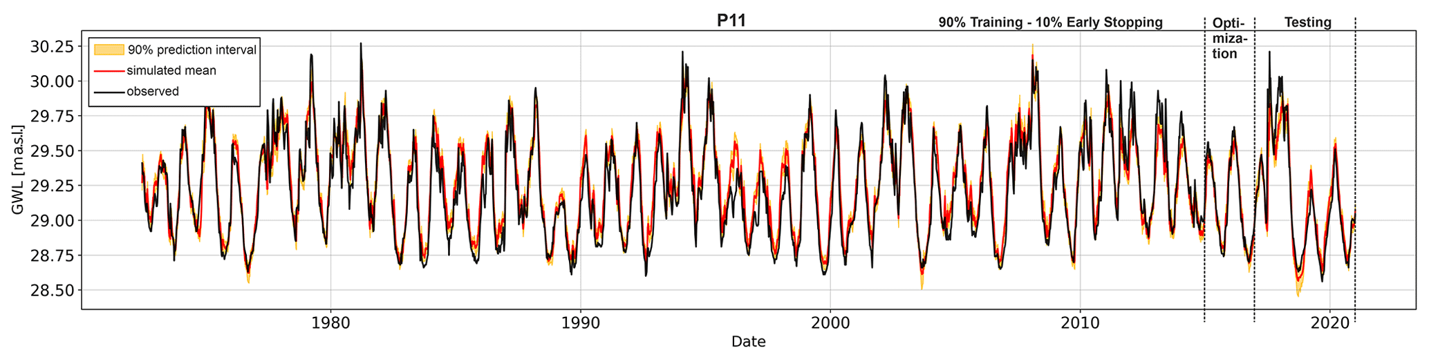
Figure 4 Model fit with high accuracy for all parts of the respective time series (location: P11; compare with Fig. 1).

2.3 Layer-wise relevance propagation

Layer-wise relevance propagation (LRP) (Bach et al., 2015) is a framework for explaining model predictions through decomposition. LRP redistributes the prediction f(x) backwards through all layers of a neural network (in our case) using local redistribution rules and assigns a relevance score R_i to each input (Samek et al., 2017); hence, in our case, a score is calculated for each value within the input sequence of both input variables, precipitation P and temperature T. LRP is also a local explanation method that explains each prediction using a single set of inputs. An important part of LRP is the conservation property, which means that each R_i of each input determines its individual contribution to the model output f(x), and no relevance is added or removed during the relevance redistribution procedure (Samek et al., 2017). LRP thus exhibits the additive feature attribution property, which means that the sum of all instances of R_i(x) equals f(x). Several redistribution or attribution rules exist, with the most basic one being the LRP_z rule, which performs a proportional decomposition and is used in this study (e.g., Kohlbrenner et al., 2020). We implement LRP using the “iNNvestigate” toolbox from Alber et al. (2019). As we use a model ensemble of 20 CNNs per location, for each individual R_i value, we investigate the mean R_i value of all 20 models for further interpretation during our analyses.

3 Results and discussion

For the following analyses, we refer to the four seasons as the 3-month periods DJF (winter), MAM (spring), JJA (summer), and SON (fall). At the investigated locations, the annual minimum usually occurs during September, which is why we distinguish between summer (JJA) and a so-called low-water period that we define as the 3 months from July to September (JAS). Besides the annual minimum, this period also nicely captures the strongest downward trends of the considered groundwater hydrographs. The corresponding high-water period, which includes the annual maximum in January or February and the strongest increasing groundwater levels of the annual cycle, aligns with the winter period and does not need a separate definition.

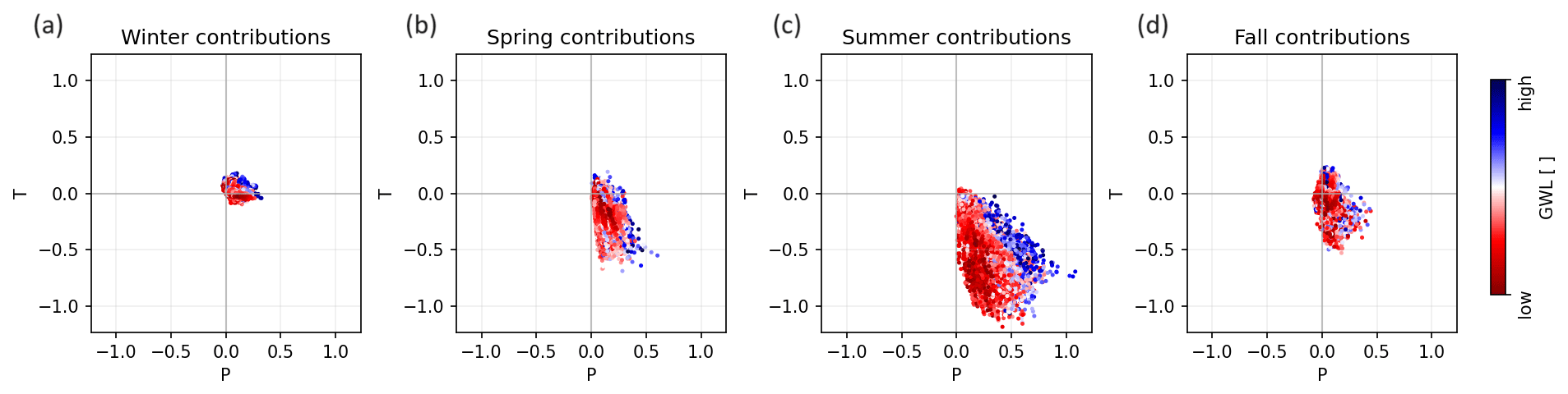
Figure 5 Influence of seasons on low-water periods expressed as relevance scores, distinguished by input variable. Each dot represents the accumulated effect of an input variable during one season on a specific low-water period.

In the following, we explore the influence of the four seasons on the low-water periods. Thanks to the additive feature attribution property of LRP, we can sum all R_i within a certain time period (here, one season) in the input sequence of a simulated groundwater level in a low-water period to estimate the effect of the whole season on the model output. The results for all low-water periods at all locations are shown in Fig. 5. For spring, summer, and fall, we mostly find negative contributions of T (i.e., higher temperatures relate to lower GWLs) and positive contributions of P (i.e., higher precipitation coincides with higher GWLs), as can be expected. We see that summer (Fig. 5c) has the largest influence (with generally high absolute relevance scores R_i) and winter (Fig. 5a) has the smallest influence on the GWLs in low-water periods, while spring and fall contributions are moderate. In winter (and in parts also in spring and fall), T predominantly contributes slightly positively, while negative contributions are subordinate. This might be explained by the correlation effects of T and P; for example, higher temperatures in winter and some periods of spring and fall are often associated with higher rainfall (or snowmelt in winter), and, especially in winter, low temperatures can be associated with either snow (which is included in P but does not directly lead to a groundwater level increase due to snow storage) or rather dry periods (Berg et al., 2009; Trenberth and Shea, 2005). The influence of summer is plausible, both in its relative strength because of the temporal proximity (overlap, even) and in its clear positive contributions of P and negative contributions of T. However, the small contribution values in winter demonstrate that the models do not learn any strong connection between winter and low-water periods, which also means that a preceding wet winter does not seem to be able to compensate for the negative influence of the summer that follows. Both spring and fall show a similarly moderate influence. The influence of fall is even higher than that of winter, despite the longer time lag, and might be related to the model learning that the conditions 1 year earlier have a certain importance. However, our approach per se cannot account for accumulative effects over several years, which is a clear limitation. Especially in summer, the influence of P can be clearly distinguished between high groundwater levels (blue dots) and low groundwater levels (red dots; i.e., a spread of red and blue dots along the P axis), while the influence of T is rather uniform. This leads to the conclusion that the models learn that summer P is the control for the severeness of a low-water period, whereas the temperature has a generally strong negative influence, but it cannot be seen that higher summer T leads to predominantly lower groundwater levels in dry periods.

In the following, we take a closer look at the generally identified influence of the input variables on groundwater levels (Fig. 6). In contrast to the analysis above, single events (data points) are shown, not sums within specific periods. The x axis represents the contribution to the model output, and the color encodes the input feature value. We find results in agreement with the analyses above, meaning that LRP identifies T as, on average, more important than P (higher mean absolute value); T is clearly responsible for negative contributions; and P contributes mostly positively to the model output. P exhibits a clear positive correlation with the relevance scores (Pearson's r=0.60, p=0.0), meaning that strong P events contribute more positively to the model output than weak events. The negative influence of T is less clear in this sense, and we find only a weak negative correlation (Pearson's $r=-\mathrm{0.14}$, p=0.0). The reason for this could be the partly contradictory role of temperature depending on the season, as already discussed in the context of the positive contributions of T in winter in Fig. 5a. In contrast to the analyses shown in Fig. 5, where the maximum relevance scores are higher for T than for P, we now look at single events, and here we clearly see that, in absolute values, strong precipitation contributes up to twice as strongly compared to temperature. Note that a few LRP relevance scores for high P inputs (dark blue) exhibit negative values. Further investigation showed that these occur predominantly with a large temporal distance to the target. This thus might be a way for the model to cope with strong precipitation events in the past that do not influence the model output positively anymore. We speculate that this might be an effect of the long input sequence that we forced the model to use, which is most certainly longer than what an optimization would have selected for the respective location.

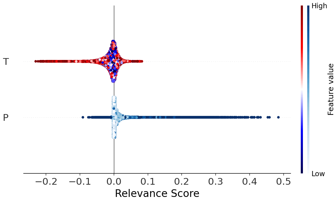
Figure 6 Summary bee swarm plots for all locations showing the learned relationships between the input variables (P, T) and groundwater levels. One dot represents 1 week at one location.

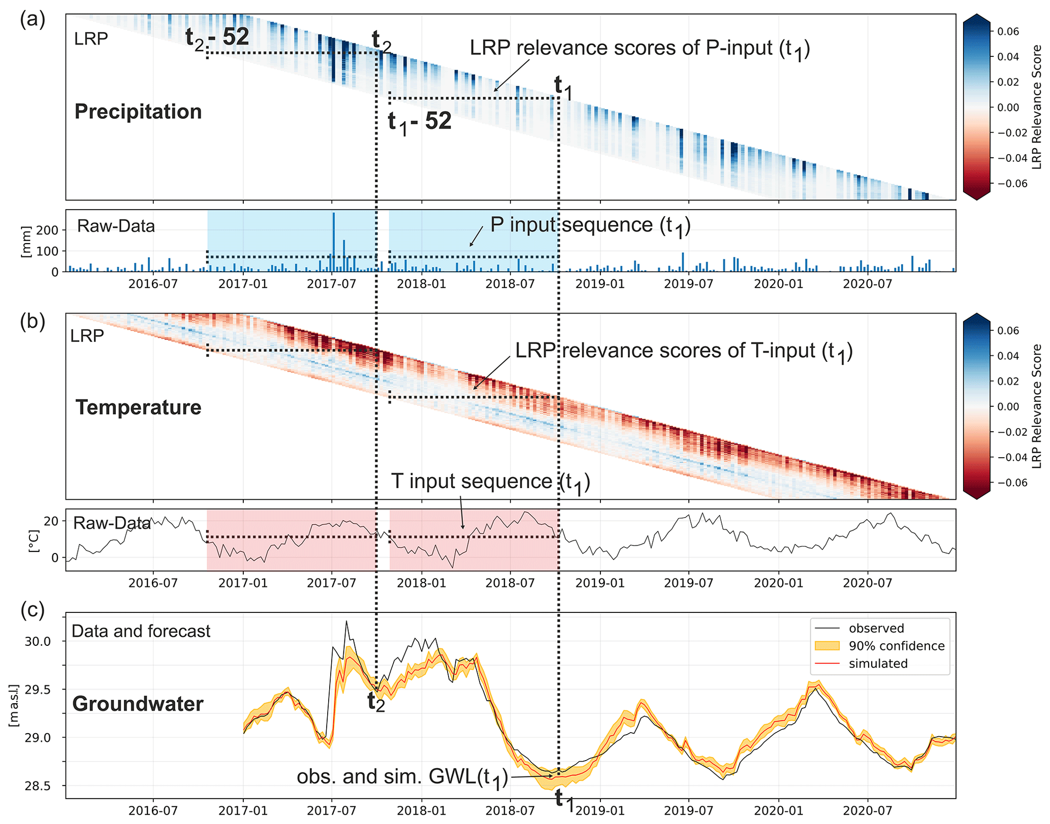
Figure 7 Breakdown of the LRP relevance scores of each variable in the input sequence within the test set (2017–2020) at location P11. All graphs are aligned in terms of time (x axis). The dashed lines indicate how to read the figure. Each forecasted GWL (c) at an arbitrary point in time (e.g., t₁ or t₂) uses an input sequence of 1 year (52 values) – compare raw data plots above in (a) and (b). Hence, each horizontal line within the LRP heatmaps for P (a) and T (b) represents the LRP relevance scores for each input value within one input sequence.

In the following, we explore the results at location P11 in detail, which, in terms of results, in many ways is a typical example from our dataset. Figure 7 shows the raw data of the former analyses, and thus the input data and corresponding LRP values, temporally ordered for the test period, and should be read as follows. (i) Panel (c) shows the observed and simulated GWLs within the test period. (ii) Each simulated GWL (e.g., at time t₁ or t₂) is based on an input sequence of 1 year (52 values). Such raw input data are displayed above in panels (a) and (b) for P and T, respectively. (iii) Additionally, heatmaps in (a) and (b) show the LRP relevance scores (dotted horizontal lines) for each input sequence from t−52 (left side) to t (right side). All panels share the same x axis and are aligned in terms of time. Corresponding figures for all other locations are part of the Supplement.

Figure 7 visualizes well how LRP relevance changes for each input value over time within the input sequence. For all P events, the heatmap of LRP values shows that blue fades out in columns from top to bottom, meaning that the importance of P events decreases with the temporal distance to the target value (right side), which is a plausible behavior. Even though some events (e.g., July 2017) do not seem to decrease, in reality they do, and this is only an effect of the upper limit of the color scale. Overall, strong events have an influence that lasts longer than that of weak events. We find that all LRP relevance scores in (a) are either positive or close to zero, while negative influences (as observed in Fig. 6) are not visible for location P11. The above-described seasonal differences in P contributions are also not clearly visible for location P11.

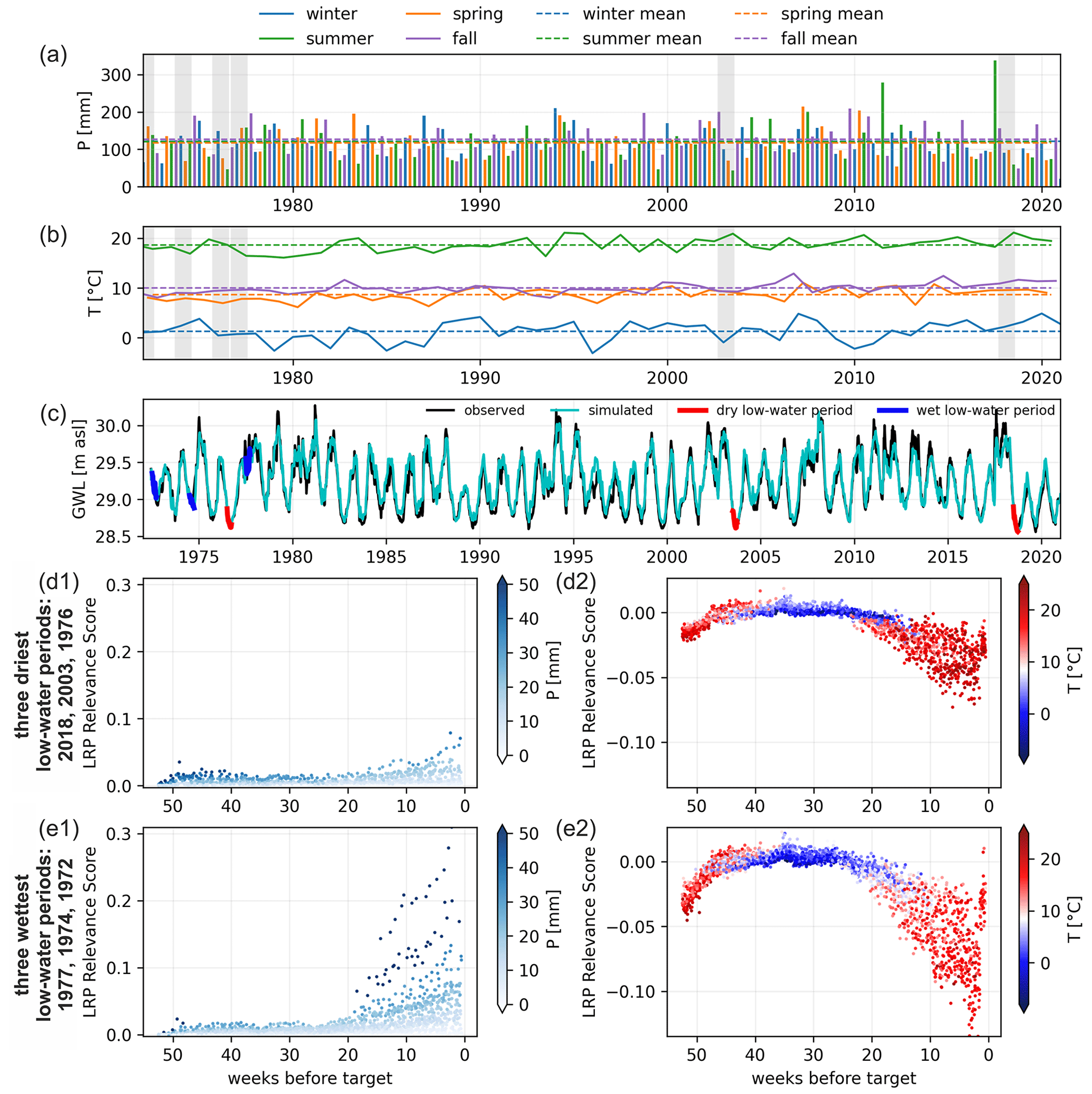
Figure 8 Seasonal P sum (a) and mean T (b) as well as observed and modeled GWLs (c) for the whole time series. LRP relevance of all input sequences for the three wettest (e) and three driest (d) low-water periods, distinguished by the input variable. Location: P11.

The second heatmap of LRP values of T inputs in (b) shows that summer T causes stronger negative contributions than winter T in the recent past, causing a periodical color pattern of dark and light red on the right side of the diagonal. In contrast, with a larger temporal distance to the target values (middle part of the diagonal), all T inputs cause neutral (white) or even slightly positive (blue) contributions. Again, summer T causes stronger LRP contributions compared to winter T; however, they are more positive in this case (white and blue diagonal). While this is only one example location, we find such patterns (summer–winter periodicity and/or negative contribution changing to positive contribution with temporal distance) regularly in our data. When investigating a particularly low groundwater level in late September 2018 (t₁) and examining the LRP values of the relevant input sequence, we find that though the temperatures were on average higher in the months before, the LRP values of T show only moderately negative influences in this time period. Rather, the temperature in the winter before has slightly lower positive influence, and there were exceptionally few precipitation events in the relevant time period. When looking at the low-water period 1 year before (t₂), which exhibits a distinctly higher groundwater level than t₁, the LRP values of T in the weeks before are much more negative but obviously were counteracted by heavy rainfall events in the summer of 2017, as is also shown by the strongly positive LRP values for P. This confirms the results shown above, indicating that summer P seems to be the most dominating factor for low groundwater levels in late-summer low-water periods.

By selecting specific periods and rearranging these LRP data, we can gain further insights into the differences between drier (most severe) and wetter (least severe) low-water periods. Figure 8 thus shows an analysis of the three wettest and three driest low-water periods at location P11. At the top of the figure, seasonal P sums (a) and T means (b) are shown, with gray bars marking the six selected periods evaluated below. Figure 8c displays observed and modeled GWLs, also highlighting the selected periods in red and blue.

Location P11 is a typical example of the low-water periods being dominated by summer P. We find considerably higher LRP values for P in the wetter low-water periods of the recent past (e1) than in the drier periods where the LRP values remain predominantly low (d1). This observation is in agreement with panel (a1), where we can see the drier periods have P sums during summer that are below the average of all years, whereas the wetter periods indeed show sums at about average (1972, 1974) or above (1977). Mean instances of summer T are mild for the wetter low-water periods, and in winter, there is no clear systematic behavior for both P and T (b). Correspondingly, the drier periods exhibit clearly below-average summer P (a), while winter P and T, again, show no systematic behavior (a, b). Interestingly, we can find stronger negative contributions in terms of T for the wetter years (d2), which might be related to the fact that evapotranspiration (with T as its proxy here) depends on water availability; thus, in wetter years, higher evapotranspiration can occur. However, the general shapes in (d2) and (e2) are similar, with strong negative values in the recent past (spring and summer), neutral values during winter (approx. between weeks 20 and 40), and slightly negative values in the distant past. Corresponding figures for all other locations are part of the Supplement to this study.

4 Conclusions

In this study, we gained insights into the influence of seasons on groundwater levels in Germany, with an emphasis on low-water periods. Layer-wise relevance propagation (LRP), a powerful XAI method, enabled us to interpret what artificial neural network models learn regarding the contribution of the two input variables, precipitation and temperature, in each season.

We found that LRP is a valuable tool not only for gaining general insights into what ANNs learn but also for disentangling such knowledge in terms of time and thus analyzing time series models. In the specific context of groundwater simulation, we found that the learned relationships do coincide well with the existing conceptual understanding of the relevant physical processes. This makes such modeling results trustworthy and also allows us to confidentially interpret yet unknown effects and relationships that can be found in the results.

We find that summer is the key season for low-GWL periods at our example locations. Especially, summer precipitation seems to control the severeness of such low-water periods in late summer, whereas higher summer T does not per se lead to lower GWLs in fall. Wetter low-water periods result from higher summer precipitation and are only subordinately related to the preceding winter season because, generally, winter exhibits only a minor influence on low-GWL periods in late summer. In summary, dry summers have a major influence on low-water periods and generate a deficit that apparently preceding wet winters cannot compensate for at the investigated locations.

In agreement with other studies (e.g., Thober et al., 2018) that indicate that lower water availability primarily originates from changes in temperature, in this study, T is identified as, on average, the more important variable. However, this seems to be the case only on average since single P events show LRP contributions that are twice as high as those of T at its maximum. The greater influence of P is especially relevant for low-water periods in late summer.

An important limitation is definitely that we focus on only two input variables – on the one hand, this allows us to disentangle effects and draw conclusions, but on the other hand, conclusions are somewhat limited. The main limitation of the approach used in this paper is, however, that it cannot account for accumulative effects over several years, as only 1 year of input data for each forecast is used and the model does not contain any kind of memory. Future research should focus on such interannual relationships and should account for such accumulative effects, which, of course, would also complicate evaluation and interpretation. This could be done, for example, by using recurrent neural networks, which contain a memory state, or replacing the whole ANN–XAI approach with a model class that has better capabilities in this sense.