the Creative Commons Attribution 4.0 License.
the Creative Commons Attribution 4.0 License.
 | 02 May 2024
Technical note: Two-component electrical-conductivity-based hydrograph separation employing an exponential mixing model (EXPECT) provides reliable high-temporal-resolution young water fraction estimates in three small Swiss catchments
Alessio Gentile
Jana von Freyberg
Davide Gisolo
Davide Canone
Stefano Ferraris
The young water fraction represents the portion of water molecules in a stream that have entered the catchment relatively recently, typically within 2–3 months. It can be reliably estimated in spatially heterogeneous and nonstationary catchments from the amplitude ratio of seasonal isotope (δ18O or δ2H) cycles of stream water and precipitation, respectively. Past studies have found that young water fractions increase with discharge (Q), thus reflecting the higher direct runoff under wetter catchment conditions. The rate of increase in the young water fraction with increasing Q, defined as the discharge sensitivity of the young water fraction (), can be useful for describing and comparing catchments' hydrological behaviour. However, the existing method for estimating , which only uses biweekly isotope data, can return highly uncertain and unreliable when stream water isotope data are sparse and do not capture the entire flow regime. Indeed, the information provided by isotope data depends on when the respective sample was taken. Accordingly, the low sampling frequency results in information gaps that could potentially be filled by using additional tracers sampled at a higher temporal resolution.
By utilizing high-temporal-resolution and cost-effective electrical conductivity (EC) measurements, along with information obtainable from seasonal isotope cycles in stream water and precipitation, we develop a new method that can estimate the young water fraction at the same resolution as EC and Q measurements. These high-resolution estimates allow for improvements in the estimates of the . Our so-called EXPECT (Electrical-Conductivity-based hydrograph separaTion employing an EXPonential mixing model) method is built upon the following three key assumptions:
-
We construct a mixing relationship consisting of an exponential decay of stream water EC with increasing young water fraction. This has been obtained based on the relationship between flow-specific young water fractions and EC.
-
We assume that the two-component EC-based hydrograph separation technique, using the above-mentioned exponential mixing model, can be used for a time-source partitioning of stream water into young (transit times < 2–3 months) and old (transit times > 2–3 months) water.
-
We assume that the EC value of the young water endmember (ECyw) is lower than that of the old water endmember (ECow).
Selecting reliable values from measurements of ECyw and ECow to perform this unconventional EC-based hydrograph separation is challenging, but the combination of information derived from the two tracers allows for the estimation of endmembers' values. The two endmembers have been calibrated by constraining the unweighted and flow-weighted average young water fractions obtained with the EC-based hydrograph separation to be equal to the corresponding quantities derived from the seasonal isotope cycles.
We test the EXPECT method in three small experimental catchments in the Swiss Alptal Valley using two different temporal resolutions of Q and EC data: sampling resolution (i.e. we only consider Q and EC measurements during dates of isotope sampling) and daily resolution. The EXPECT method has provided reliable young water fraction estimates at both temporal resolutions, from which a more accurate discharge sensitivity of the young water fraction () could be determined compared with the existing approach. Also, the method provided new information on ECyw and ECow, yielding calibrated values that fall outside the range of measured EC values. This suggests that stream water is always a mixture of young and old water, even under very high or very low wetness conditions. The calibrated endmembers revealed a good agreement with both endmembers obtained from an independent method and EC measurements from groundwater wells.
For proper use of the EXPECT method, we have highlighted the limitations of EC as a tracer, identified certain catchment characteristics that may constrain the reliability of the current method and provided recommendations about its adaptation for future applications in catchments other than those investigated in this study.
- Article
(8215 KB) - Full-text XML
-
Supplement
(707 KB) - BibTeX
- EndNote


Environmental tracers in catchment studies are used to understand the age, origin and pathways of water in natural environments (Kendall and McDonnell, 1998). Among tracers, hydrologists use the stable water isotopes (18O and 2H) because they are a constituent part of water molecules and, thus, are naturally present in precipitation (Kendall and McDonnell, 1998). The isotopic composition of precipitation (CP) generally shows a pronounced seasonal cycle (Dansgaard, 1964). Catchment storage acts as a filter on this seasonal input cycle, so that the isotope cycle in stream water (CS) is damped and lagged compared with that of precipitation (McGuire and McDonnell, 2006). The delay and damping that we observe in the stream water cycle is caused by the advection and dispersion of stable water isotopes that reach the catchment with precipitation, thus reflecting water mixing as well as the diversity of flow paths and their velocities (Kirchner, 2016a; McGuire and McDonnell, 2006).
Kirchner (2016a, b) proposed a new water age metric directly related to the amplitude ratio of the seasonal isotope cycles in stream water and precipitation: the young water fraction, i.e. the portion of runoff younger than roughly 2–3 months. The precipitation isotope cycle amplitude (AP) is generally estimated via a robust fit of a sine function to the isotopic composition of precipitation samples using the precipitation amount associated with each sample as the weight to reduce the influence of low-precipitation events (von Freyberg et al., 2018a; Kirchner, 2016a). The stream water isotope cycle amplitude is estimated via a robust fit of a sine function to the isotopic composition of stream water samples with or without using discharges (Q) at the sampling times as weights (von Freyberg et al., 2018a). Please note that, hereafter, the symbol “*” indicates a streamflow-weighted variable. Therefore, it is necessary to distinguish between the unweighted and the flow-weighted stream water amplitude (AS and , respectively; see Eq. (S2) for further details) and, accordingly, between the unweighted and the flow-weighted young water fraction (Fyw and , respectively).
Recently, Gallart et al. (2020b) proposed a method to estimate the rate of increase in the young water fraction with increasing Q by fitting the sinusoid function, with amplitude , directly to the isotopic data of stream water as follows:
where the , , and parameters are obtained via non-linear fitting (see “The discharge sensitivity of young water fraction” section in the Supplement for additional methodological details). The (d mm−1) parameter is defined as the discharge sensitivity of the young water fraction, (–) is the virtual young water fraction when Q=0, (rad) is the phase of the seasonal cycle, f is the frequency (equal to once per year for a seasonal cycle) and (‰) is a constant representing the vertical offset of the seasonal cycle. Referring to the expression enclosed in square brackets in Eq. (1), the young water fraction is assumed to vary with discharge following an exponential-type equation that converges toward 1 at the highest flows but that does not converge toward 0 at the lowest flows, thus theoretically admitting . Because of this mathematical relationship between the young water fraction and Q, young water fraction time series can, in theory, be calculated at the same temporal resolution as Q. However, the uncertainties in such time series can be substantial because the underlying isotope data, due to the low sampling frequency, are generally not able to capture the entire range of flow regimes, especially the (very) high flow rates (Xia et al., 2023). This becomes evident in Figs. 1 and 3 of Gallart et al. (2020b), where the standard errors of flow-specific Fyw are largest during the highest flows. From these considerations emerges the need for a new method to reliably estimate the time series of young water fractions and to better constrain the discharge sensitivity of young water fractions under very low and very high flow conditions.
Multiyear stable water isotope data sets are typically available at relatively low (e.g. biweekly or monthly) temporal resolutions because of the high cost of sampling and laboratory analysis (Mosquera et al., 2018). For the same reasons, high-resolution isotopic data sets are often limited to relatively short time windows (Wang et al., 2019). However, the information provided by isotope data depends on when the respective samples were taken (Wang et al., 2019). Consequently, sampling at low temporal resolution results in information gaps that could potentially be filled by using additional tracers sampled at higher temporal resolution. As a tracer, electrical conductivity (EC), which is a bulk measure of the major ions in water (Riazi et al., 2022), can be measured over extended periods at high temporal resolution, while the cost of installation and maintenance remains low (Cano-Paoli et al., 2019; Mosquera et al., 2018). However, EC is not a conservative tracer (like stable water isotopes) because it is affected by geochemical reactions and the dissolution of reactive solutes in stream water (Cano-Paoli et al., 2019; Benettin et al., 2022). Because of these characteristics, the EC and stable water isotope tracers complement each other well and, thus, can be jointly used to constrain model parameterizations and to inform transit time models (Cano-Paoli et al., 2019; Benettin et al., 2022).
A time-source separation is generally performed using isotope hydrograph separation, IHS (Klaus and McDonnell, 2013), while major ions (approximated by EC) have been previously used for geographic-source separation in endmember mixing analysis (Hooper, 2003; Penna et al., 2017). Major ions' concentration in stream water derives from mineral weathering. Weathering processes can be viewed as a series of geochemical reactions influenced by the characteristics of fluid movement, such as the contact time between the flowing water and mineral surfaces (Benettin et al., 2015, 2017). Thus, the longer a water particle remains within the subsurface, the higher its solute concentration (and thus EC) will be once it is released as streamflow (Benettin et al., 2017). Indeed, Mosquera et al. (2016), investigating the mean transit time (MTT) of water and its spatial variability in the wet Andean páramo, found that the mean EC is an efficient predictor of mean transit time in this high-elevation tropical ecosystem. More recently, Riazi et al. (2022), modelling EC variation using a travel time distribution approach, assumed that the salinity of water in catchment storages is a function of water age. Bonacci and Roje-Bonacci (2023) used EC measurements of a karst spring to estimate the time that water spent in the karst aquifer. In addition, Kirchner (2016b) stated that the concentration of reactive chemical species, such as EC, can be used to construct a mixing relationship with the young water fraction, which provides information about the water age. Overall, these studies suggest that EC may provide useful information on water age (Riazi et al., 2022). Indeed, past studies have used EC for time-source hydrograph separation (HS) in event and pre-event water with promising results that favourably compare with those obtained from conservative tracers (Riazi et al., 2022). For instance, Laudon and Slaymaker (1997), applied HS in two small nested alpine/subalpine catchments using different tracers (δ18O, δ2H, EC and silica) and returned generally comparable results overall. Cey et al. (1998), with the aim of quantifying groundwater discharge in a small agricultural watershed, separated the hydrograph into event and pre-event water (assumed to be groundwater), obtaining only slightly different results utilizing δ18O and EC. Pellerin et al. (2008) performed HS on 19 low- to moderate-intensity rainfall events in a small urban catchment via the use of EC, silica and δ2H, obtaining a similar outcome regardless of the tracer used. In a similar environment, Meriano et al. (2011) revealed a high level of agreement between flow partitioning results during a midsummer event using HS with δ18O and EC as tracers. Camacho Suarez et al. (2015), to identify the mechanisms of runoff in a semi-arid catchment, applied HS using both EC and δ18O and found no major disadvantages when using EC. More recently, Mosquera et al. (2018) used the TraSPAN model to simulate storm flow partitioning in a forested temperate catchment, revealing similar portions of pre-event water regardless of the tracer (δ18O and EC) used. Cano-Paoli et al. (2019), by investigating the streamflow separation into event and pre-event components in an alpine catchment, obtained consistent results using δ18O, δ2H and EC. Lazo et al. (2023) showed that, in a tropical alpine catchment, the use of EC returned similar results for event and pre-event water to those obtained with δ18O for a wide range of flow conditions reflected by the 37 monitored rainfall–runoff events. Overall, the findings of these studies suggest a quasi-conservative behaviour of EC under a wide range of hydrological and lithological conditions, even if its behaviour depends on specific characteristics (e.g. water partitioning between the surface and the subsurface, spatial distribution of minerals and subsurface properties, kinetics of rock dissolution, and individual ion concentrations) of each watershed (Laudon and Slaymaker, 1997; Benettin et al., 2022; Lazo et al., 2023). Nevertheless, these studies have been limited to the comparison of results obtained by applying HS with different tracers and did not integrate the information obtainable from stable water isotopes and EC to generate new insights into transit times, hydrological processes, or the links between water quality and water age variations (Benettin et al., 2017, 2022).
In this regard, here we develop a new multi-tracer method that combines biweekly stable water isotope data (δ18O) with EC measurements. This study aims to both reduce the standard error of and estimate the young water fraction at a temporal resolution higher than 2 weeks, which will lead to new insights into the catchments under study.
2.1 Study sites and the data set
To test the applicability of our method (Sect. 2.2), we use data from the Erlenbach (ERL), Lümpenenbach (LUE) and Vogelbach (VOG) catchments, located in the pre-alpine Alptal Valley in central Switzerland. The geographical framework of the three study sites is reported in Fig. 1.
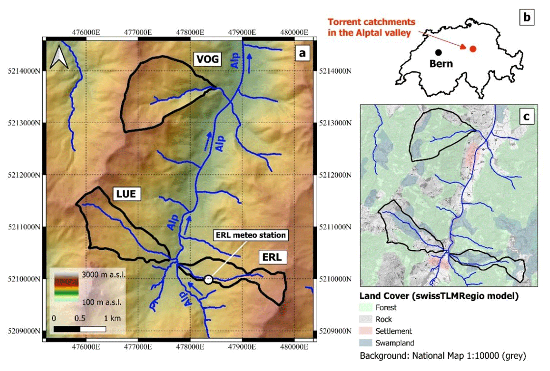
Figure 1(a) Location of the three study catchments with indication of the stream networks and elevation (DHM25 © swisstopo) as background. The Alp River is marked in the map with blue arrows indicating its flow direction. (b) Location of the Alptal Valley in Switzerland. (c) Land cover of the three study catchments from the swissTLMRegio 2D landscape model (© swisstopo).
The three study catchments cover areas of between 0.7 and 1.6 km2, and mean elevation ranges from 1335 to 1359 m a.s.l. (metres above sea level; Table 1, Fig. 1a). Mean catchment slopes are 13.53, 12.49 and 18.42° in the ERL, LUE and VOG catchments, respectively, but the hillslopes can be much steeper locally (20–40°) (Stähli et al., 2021). According to the swissTLMRegio model (Fig. 1c), the ERL catchment is mainly constituted by forest (45 %) and swampland (49 %); these are also the dominant classes in the LUE (21 % and 39 %, respectively) and VOG (72 % and 13 %, respectively) catchments. Most of the southern Alptal Valley is characterized by shallow, low-permeability Gleysols that limit the deep infiltration of water and lead to shallow groundwater tables (Stähli et al., 2021). The percentage of soils with a low storage capacity is about 4 % in both ERL and LUE, while it is 51 % in the VOG catchment; a large fraction of the soils is saturated (≥95 % in ERL and LUE and 49 % in VOG; von Freyberg et al., 2018a). The geological substratum of the three study sites consists mainly of sedimentary rock (flysch). The catchment area that is covered by Quaternary deposits is much higher in the ERL and LUE catchments than in the VOG catchment (Table 1). Therefore, although the study catchments are located within close proximity, they differ in terms of soil wetness and unconsolidated sediments.
Table 1Topographic, geological and hydro-climatic properties of the three study sites.
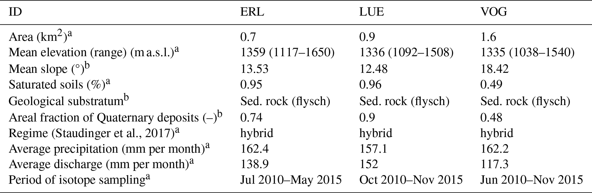
a Data published in von Freyberg et al. (2018a). b Data published in Gentile et al. (2023).
The average hydro-climatic conditions are generally similar for all three catchments. The average annual precipitation in the period from January 2000 to December 2015, based on interpolated data from the PREVAH model, was about 1853, 1803 and 1800 mm in the ERL, LUE and VOG catchments, respectively (von Freyberg et al., 2018a). The average monthly discharge is similar among the catchments: 138.9, 152.0, and 117.4 mm per month at the ERL, LUE and VOG catchments, respectively (von Freyberg et al., 2018a). These watersheds reveal a hybrid hydro-climatic regime (Staudinger et al., 2017; von Freyberg et al., 2018a), as we observe ephemeral snowpack formation (typically from December to April) that also rapidly melts away during winter, meaning that the snowpack may not last throughout the entire winter season (Stähli et al., 2021).
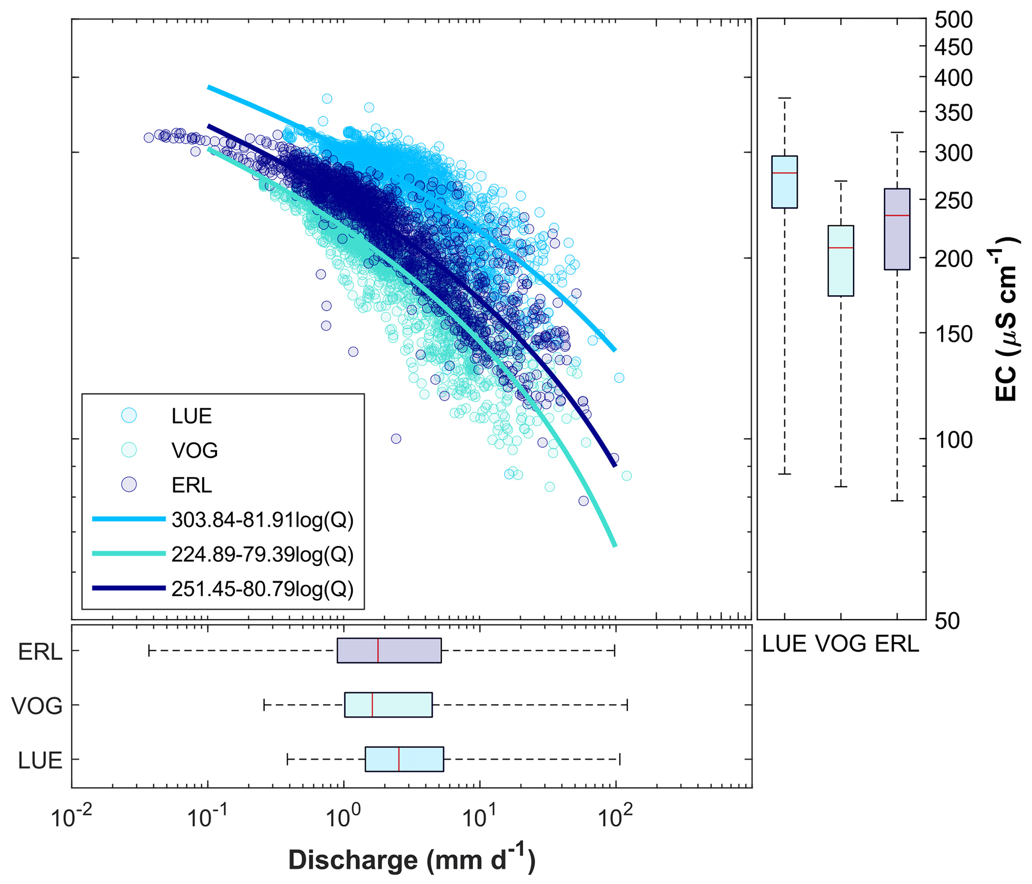
Figure 2Relation between daily EC and daily Q for the three study sites. As discharge increases, the EC decreases in the three study catchments. This pattern arises mainly due to the age (source) of water contributing to the stream: if a substantial amount of recent, low-EC water contributes to streamflow during rainfall or snowmelt, stream water EC decreases while discharge increases.
Daily-resolution Q and stream water EC data have been downloaded from the Swiss Federal Office for Forest, Snow and Landscape Research (WSL, Birmensdorf, Switzerland) data portal. We have estimated the Q–EC relationships with a log-type fit (Fig. 2). As daily Q increases, daily EC decreases at the three study sites. This pattern arises due to the contribution of different sources (i.e. ages) of water to the stream. At the three study sites, stream discharge increases due to rainfall or snowmelt, which are generally low in EC, resulting in a dilution of stream water EC. In addition, during wet conditions (high Q), more rapid flow paths are activated, leading to a prevalence of the younger hydrograph component. Because of the short interaction time with mineralized rocks and soils, young water can be assumed to be low in dissolved ions (i.e. low EC). The other extreme, low Q and high stream water EC, occurs during baseflow conditions when the stream is mainly fed by old (i.e. highly mineralized and high-EC) subsurface water (Schmidt et al., 2012).
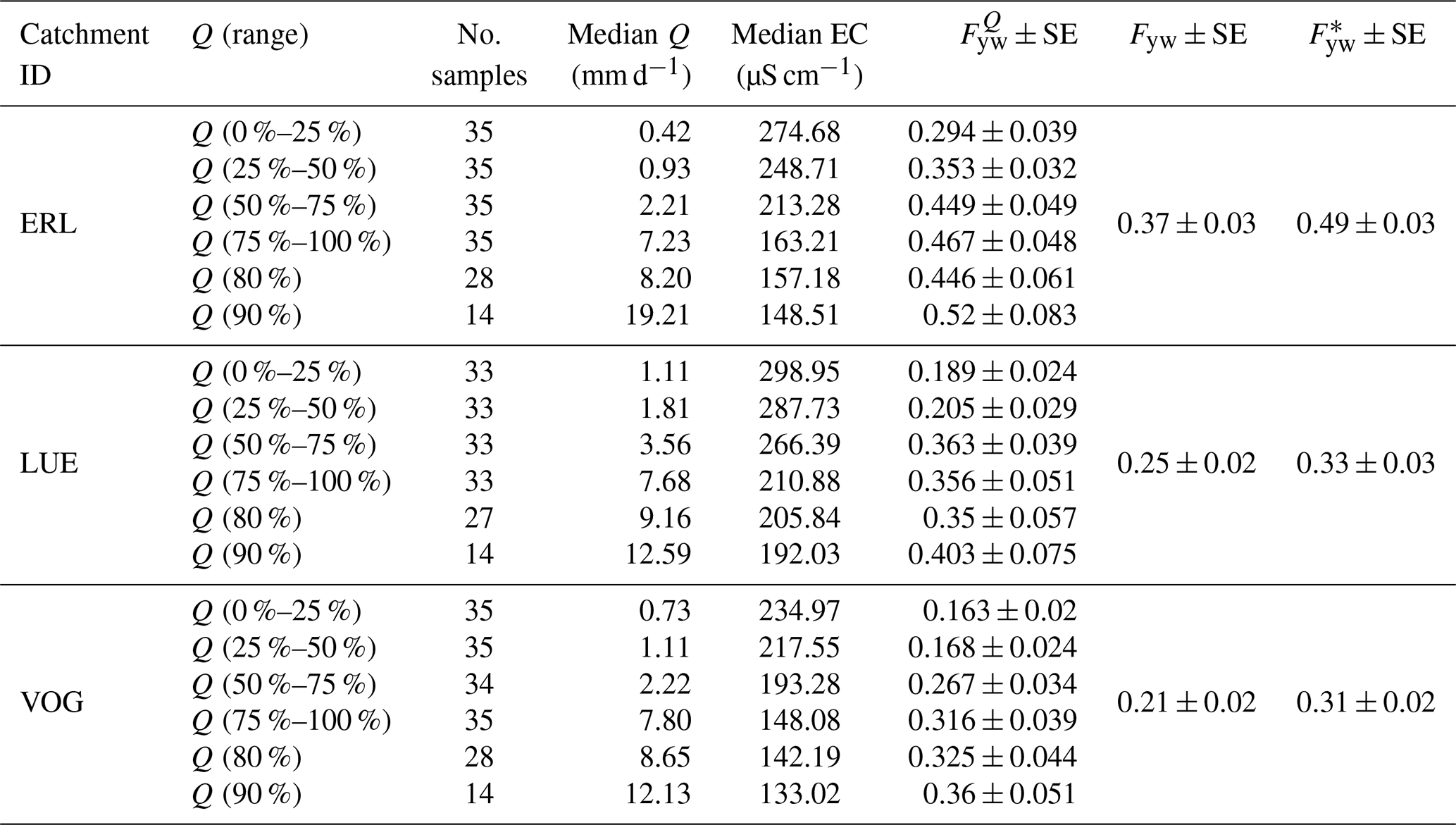
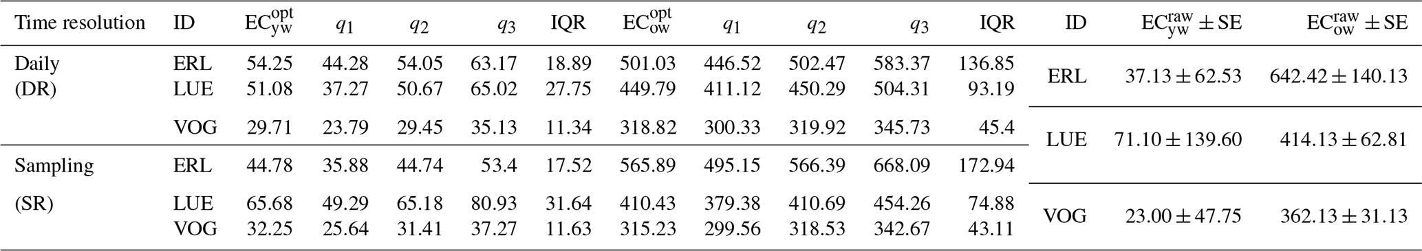
This study uses Fyw, , and (Tables 2, 4), which have been estimated in past studies (Gallart et al., 2020b; von Freyberg et al., 2018a) by considering streamflow δ18O data from biweekly grab sampling over a period of approximately 5 years for the three study catchments. values refer to young water fractions estimated in discrete flow regimes (Kirchner, 2016b). Indeed, it is possible to separate the stream water isotope data collected into different discharge ranges and fit sinusoids separately to the isotope content in each range. For each of these individual flow regimes, this method enables one to obtain the stream water seasonal isotope cycles amplitude () values that will be divided by AP to obtain (von Freyberg et al., 2018a; Kirchner, 2016b). For more details about estimation, the reader is referred to Kirchner (2016b) and von Freyberg et al. (2018a).
Table 2Young water fractions of distinct flow regimes () as well as average unweighted and flow-weighted young water fractions (Fyw and , respectively) with the corresponding standard error (SE) values. The number of samples used to estimate alongside the median Q and EC of each flow regime are also reported. These data, excluding the median EC, were previously obtained by von Freyberg et al. (2018a).
2.2 The EXPECT method: two-component electrical-conductivity-based hydrograph separation employing an exponential mixing model
The young water fraction may be useful for inferring chemical processes from streamflow concentrations of reactive chemical species (Kirchner, 2016b). Indeed, as it is known how the fraction of young water varies in discrete flow regimes, it is possible to construct mixing relationship between and the concentration of reactive chemical species (Kirchner, 2016b). Accordingly, we calculate the median EC within each individual discharge range (reported in Table 2), and we investigate how the median EC varies with (Fig. 3).
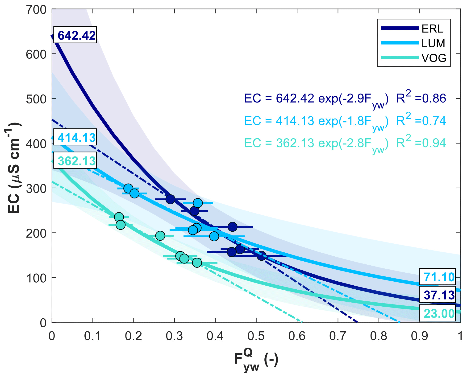
Figure 3Median-flow-specific EC against for the three study catchments. Horizontal bars indicate the standard error. The solid lines indicate the exponential fits (for which expressions with the corresponding R2 value are also indicated). The shaded areas indicate the 90 % prediction bounds. The text boxes corresponding to indicate a first-order estimate of old water endmembers (EC) using the exponential expression. Similarly, the text boxes corresponding to indicate a first-order estimate of young water endmembers (EC) using the exponential expression. The dashed lines indicate the linear fits to data that point to a negative EC endmember of young water (i.e. EC value corresponding to ).
As visible in Fig. 3, the relationship between and median-flow-specific EC is well described by an exponential mixing model. Indeed, the widely used linear mixing model proves to be poorly suited here because it is pointing to a negative EC endmember of young water (i.e. EC value corresponding to ; Fig. 3). This will be thoroughly discussed in Appendix A. By considering the exponential mixing model, we can estimate the “idealized” old water and young water endmembers via evaluation of the fitted exponential expressions for and , respectively. Accordingly, a first-order estimate of the two endmembers (EC EC, respectively) is reported in Fig. 3 and Table 3. It is evident that the measured for the three study catchments ranges from approximatively 0.1 to 0.5 (Fig. 3). As the measurable range of young water fractions is not wide enough, the parameters estimated with the exponential fit are highly uncertain because the curve is poorly constrained at very low (<0.1) and very high (>0.5) young water fractions. In this regard, hereafter, we propose a new methodology to estimate the EC endmembers of young and old water, respectively, and to perform a continuous hydrograph separation with an alternative mixing model.
Table 3Optimized endmembers obtained via the EXPECT method. The 1st, 2nd and 3rd quartiles (q1, q2 and q3, respectively) and the interquartile range (IQR) of the optimized endmembers' empirical distribution are also reported. First-order estimates of endmembers derived from the exponential model fitted on median EC vs. (see also Fig. 3) with the related standard error (SE) values are reported on the right-hand side of this table. Values are in µS cm−1.
The definition of the fraction of the streamflow younger than a threshold age (varying modestly from 2 to 3 months) at the generic time ti, Fyw(ti), implicitly defines the existence of a complementary fraction of streamflow older than that threshold age at the same time ti, Fow(ti). Thus, mass conservation requires the following:
To estimate Fyw(ti), and thus Fow(ti), we use EC as a tracer to separate the hydrograph into young (transit time < 2–3 months) and old (transit time > 2–3 months) water. Solid support from the scientific literature justifying the use of EC for time-source hydrograph separation is illustrated in Sect. 1.
As suggested by the analysis reported in Fig. 3, to perform the hydrograph separation, we assume that stream water EC at the generic time ti, EC(ti), decreases exponentially with increasing Fyw(ti):
where ECow is the old water EC endmember and a is a parameter. The exponential decay proposed in Eq. (3) guarantees a realistic scenario for the case Fyw(ti)=0, i.e. streamflow contains only old water (Fow(ti)=1) and stream water EC is equal to ECow(EC(ti)=ECow). Conversely, if Fyw(ti) is equal to 1, streamflow is made up entirely of young water. Accordingly, we can include the following condition: if Fyw(ti)=1, EC(ti)=ECyw, where ECyw is the young water EC endmember (Eq. 4),
Furthermore, we assume ECyw<ECow. Solid support of this assumption from the scientific literature is illustrated in Sect. 3.1 alongside the discussion of the results.
By further considering the law of water mass conservation (Eq. 2), it is possible to solve the system of three equations (Eqs. 2–4) with three variables (a, Fyw(ti) and Fow(ti)), thus obtaining the explicit expression of a (Eq. 5) and, accordingly, of Fyw(ti) (Eq. 6).
The main difficulty in applying Eq. (6) to estimate Fyw(ti) is that we generally cannot accurately determine the endmembers ECyw and ECow from the analysis reported in Fig. 3 or from measurements. Indeed, such endmembers correspond to the (rare) scenarios in which Fyw(ti) is either 0 or 1. The first scenario (Fyw(ti)=0) might occur only after prolonged periods without rainfall or snowmelt, whereas the second scenario (Fyw(ti)=1) is unlikely to occur in most natural catchments where baseflow is usually older than 3 months (Gentile et al., 2023), and thus we cannot directly measure ECyw (Kirchner, 2016b). In this regard, hereafter, we present a novel methodology to estimate the endmembers. Such a methodology lays its foundations on the statement that the isotope-based Fyw and (Eqs. 7a and 7b; see the Supplement for further details) accurately estimate the unweighted and the flow-weighted average young water fractions in streamflow, respectively (Kirchner, 2016b).
Accordingly, if we know the young water fraction over a generic time step ti, Fyw(ti) (e.g. daily young water fraction), we can calculate the unweighted and the flow-weighted average young water fraction in streamflow using Eqs. (8a) and (8b), respectively:
where n is the number of time steps (e.g. days) in the period of isotope sampling and Q(ti) is the discharge at the time ti(e.g. daily discharge). The hat “ ” symbol is simply used to visually differentiate between the average young water fractions obtained with both approaches. Note that Eq. (8b) was previously presented in Gentile et al. (2023).
We therefore determine ECyw and ECow through calibration, respecting the following three constraints:
- i.
ECow and ECyw are greater than or equal to 0;
- ii.
, where Fyw(ti) is obtained using Eq. (6), must match the Fyw estimated with the amplitude ratio technique (Eq. 7a);
- iii.
, where Fyw(ti) is obtained using Eq. (6), must match the estimated with the amplitude ratio technique (Eq. 7b).
In summary, we perform a constrained EC-based hydrograph separation in which the two endmembers (ECyw and ECow) are calibrated through an optimization procedure. Specifically, we use the MATLAB fmincon solver, specifically the sqp (sequential quadratic programming) algorithm, within the GlobalSearch procedure that repeatedly runs the local solver to generate a global solution. To satisfy point (i), we search the endmember values within the range [0, +∞). We consider ∞ as the upper limit because catchments can also have immobile storages that could potentially never participate to the water cycle (Staudinger et al., 2017). In addition, we calibrate the EC endmembers by minimizing the following objective function, which is designed to satisfy points (ii) and (iii):
We give a greater weight to the second term, . The weight is proportional to how much higher is than Fyw, as Gallart et al. (2020a) showed that the flow-weighted analysis produces a less biased estimation of the young water fraction. The outputs of the optimization procedure are the calibrated young water and old water endmembers (EC and EC, respectively). Subsequently, we calculate the (at every time step ti) with Eq. (6) by using the optimal endmembers (EC and EC), and we plot against Q, thereby visualizing an empirical relationship between the two variables. Finally, we fit the expression enclosed in square brackets in Eq. (1) (corresponding to Eq. 6 from Gallart et al., 2020b) to our data:
We then compare the discharge sensitivity, , previously determined using only stream water isotope data (see Eq. 1), and the discharge sensitivity, , determined from Eq. (10). We further compare our results to the values (Table 2) previously obtained by von Freyberg et al. (2018a).
We apply our method at two different time resolutions that are reflected in our data set: the daily resolution (DR) and the sampling resolution (SR). At the DR, EC(ti) and Q(ti) refer to the daily average EC and Q values, respectively; thus, Fyw(ti) is the average young water fraction of each day. At the SR, it should be noted that the “EC samples” are not referring to physical samples in this specific application. Accordingly, EC(ti) and Q(ti) are obtained by sub-setting those EC and Q values from the daily time series that correspond to the time of isotope sampling. In this sense, we can say that the number of EC samples and isotope samples is the same. Nevertheless, the method can be potentially applied at the SR in catchments in which EC is only measured from water samples. At the SR, Fyw(ti) values are estimated only for those days on which an isotope sample was taken.
We quantify the uncertainty in EC and EC by repeating the global optimization procedure by randomly sampling 10 000 couples of Fyw and from the intervals Fyw ± SE and ± SE, respectively. The SE values are reported in Table 2. The random sampling assumes that the values within the two intervals have a Gaussian probability of extraction, thus favouring the sampling of the core values. Therefore, we obtain 10 000 couples of endmembers for which we compute statistics. We further calculate the uncertainty in : we apply Eq. (6) using the 10 000 couples of endmembers, thus obtaining 10 000 values at each time step ti, for which we calculate the standard deviation.
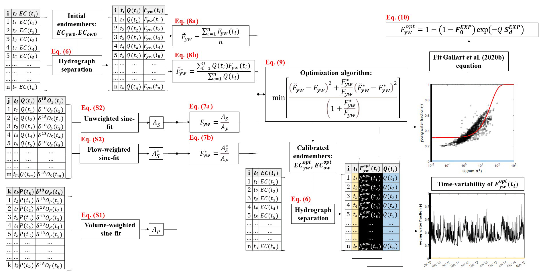
Figure 4Schematic representation of the EXPECT method. The subscript “P” refers to precipitation, while the subscript “S” refers to stream water. P(tk) indicates the volume of precipitation used for the volume-weighted fit of precipitation isotopes (δ18OP(tk)). The sampling times of EC(ti), Q(ti), δ18OS(tj) and δ18OP(tk) may not be aligned; consequently, the time series typically have different lengths. Thus, the times ti, tj and tk have different indices and usually .
It should be noted that the initial conceptualization of the mixing model was based on testing the hydrograph separation using the two-component endmember linear mixing approach with EC as the tracer (e.g. Cano-Paoli et al., 2019). As could already be inferred from Fig. 3, this approach was not successful because it can represent only a limited hydrological behaviour of catchments that does not capture that of our three study catchments. A detailed explanation of the limits regarding the linear mixing model is provided in Appendix A of this paper.
Last but not least, as our method consists of a two-component Electrical-Conductivity-based hydrograph separaTion employing an EXPonential mixing model, we decide to name it EXPECT. A schematic representation of the EXPECT method is reported in Fig. 4.
3.1 Physical likelihood of calibrated endmembers and the discharge sensitivity of the young water fraction
The application of the EXPECT method showed, at both the daily and sampling resolutions, that the old water EC endmembers, EC, are about 1 order of magnitude larger than the young water EC endmembers, EC, for all three experimental catchments (Table 3, Fig. 5). This result can be explained by considering that old water had a longer contact period with mineral surfaces in the subsurface (Benettin et al., 2015, 2017); thus, weathering-derived solute concentrations (and, correspondingly, EC) will be higher in old water compared with young water. Moreover, young and old stream water components can originate from different reservoirs in a catchment (Riazi et al., 2022). Among these reservoirs, old water is generally assumed to represent groundwater. This is also supported by the fact that the fraction of baseflow (representing the groundwater contribution to streamflow) was found to be complementary to the young water fraction in the framework (including the three Swiss catchments in this study) investigated by Gentile et al. (2023). In this regard, different papers that have characterized groundwater EC have shown notable differences with the EC of precipitation and/or meltwater. Indeed, Zuecco et al. (2018), by investigating the hydrological processes in an alpine catchment, found that the EC of rainwater and of recent snow was 19.2 and 12.2 µS cm−1, respectively. Conversely, they found that groundwater from springs had an EC of 166 µS cm−1. Moreover, by investigating the conceptualization of meltwater dynamics in an alpine catchment through hydrograph separation, Penna et al. (2017) defined the snowmelt endmember range as 2.9–15.3 µS cm−1, the glacier melt endmember range as 2–2.7 µS cm−1 and the groundwater endmember range as 210–317.7 µS cm−1 (average values from springs or streams in fall/winter). These examples are intended to show that groundwater (the main source of old water) generally reveals an EC value that is much higher (around 10- to 100-fold) than other sources in a catchment that should preferentially contribute to the young stream water component. Differences in young and old water EC endmembers can also be partially justified by looking at differences in event and pre-event water EC endmembers. Indeed, old (transit times > 2–3 months) water is a large fraction of pre-event (transit times > a few days) water, whereas event water (transit times < a few days) is a portion of young water (transit times < 2–3 months). Due to this overlap, a similarity in the old water and pre-event water EC endmembers or in the young water and event water EC endmembers would not be surprising. Cano-Paoli et al. (2019) used stream water EC to investigate hydrological processes in alpine headwaters by separating the hydrograph into event and pre-event water. In this regard, they defined the event water endmember as being equal to 8 µS cm−1 (Penna et al., 2014) and the pre-event water endmember as being equal to 95 µS cm−1 (the mean value during baseflow conditions). Laudon and Slaymaker (1997), by investigating the hydrograph separation using EC at the lower station of an alpine catchment, defined the rainwater EC endmember as being equal to 6.15 µS cm−1 and the pre-event water endmember as being equal to 39 µS cm−1. However, young and old water EC endmembers are expected to be higher than event and pre-event water EC endmembers, respectively. Accordingly, these past results taken from the scientific literature support our assumption that ECyw<ECow.
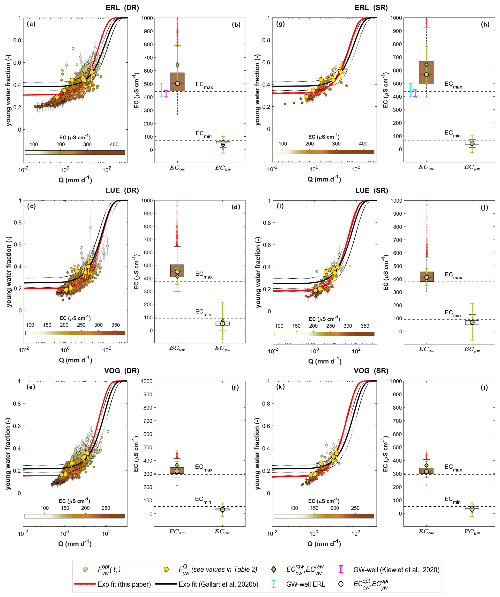
Figure 5The –Q(ti) relation for the ERL, LUE and VOG study catchments at the daily resolution (DR, a, c, e) and sampling resolution (SR, g, i, k) as well as the corresponding EC endmembers (b, d, and f and h, j, and l, respectively). The white–brown colour gradient of the points indicates the EC(ti) value. For comparison, average values of specific flow ranges (Table 2) are shown in yellow with related standard errors (yellow bars). The black curve represents the exponential-type fit using the parameters and previously obtained via non-linear fitting of Eq. (1) to stream water isotope data from Gallart et al. (2020b). The red curve represents the exponential-type fit using the parameters and obtained in this study via non-linear fitting of Eq. (10) to vs. Q. Black and red dashed lines indicate ±1 SE (standard error). Panels (b), (d), (f), (h), (j) and (l) show the box plots of EC and EC derived from the endmember uncertainty analysis. The white dots indicate the optimal endmembers (obtained by constraining the EC-based hydrograph separation using Fyw and ) used to calculate via Eq. (6). EC and EC (with the related SE values, green bars) have been superimposed for validation purposes along with the measured EC range in two groundwater wells within (solid cyan line) and near (solid magenta line) the ERL catchment. The dashed black lines, labelled ECmax and ECmin, refer to the respective maximum and minimum EC values measured in the stream.
The highest EC values were obtained for ERL (501 µS cm−1, DR), whereas the lowest values were obtained for VOG (319 µS cm−1, DR). The EC values are in line with those measured in groundwater (Fig. 5). In a 6.8 m deep monitoring well at the ERL meteorological station, groundwater EC generally varies between 400 µS cm−1 (spring–summer) and 500 µS cm−1 (fall–winter; data not shown), whereas the EC in groundwater at up to 1.5 m depth was generally around 400–450 µS cm−1 during no-snowmelt conditions in the neighbouring catchment of ERL (Kiewiet et al., 2020). The optimal endmembers are also in line with the first-order estimates of endmembers, EC and EC, derived from the exponential model fitted on median EC vs. (Table 3; Figs. 3, 5), except for ECow in the ERL catchment. This can be explained by considering the high standard error (Table 3) of the parameter (corresponding to EC) in the exponential model that is poorly constrained for ERL (more than for LUE and VOG) at low young water fractions (Fig. 3). The optimized EC values of the young water fractions appear slightly elevated compared with data derived from central European precipitation (Monteith et al., 2023). However, it is plausible to posit that the young water fraction encompasses some soil water with higher EC.
Figure 5 shows further that the interquartile range (IQR) values of the EC empirical distributions are much larger than those of EC. Assuming that the solute concentration in stream water increases with water age (Riazi et al., 2022), this can possibly be explained by the much wider range of transit times (from approximately 0.2 to tending to infinity years) of old water compared with young water (0 to 0.2 years). Consequently, the concentrations of weathering-derived solutes in old water are not only higher but also more variable than in young water.
Our method estimates the EC endmember values for the cases Fyw(ti)=1 and Fyw(ti)=0 that are generally difficult to determine experimentally, thus providing additional information about young and old water in the systems under study. In this regard, at each one of the three study sites, the theoretical endmembers EC are lower than the minimum EC value measured in the streams; analogously, the calibrated EC values are higher than the maximum measured EC value (box plots vs. horizontal dashed lines in Fig. 5). This is expected for a natural, heterogeneous system in which incoming precipitation mixes with stored water, and thus stream water never contains 100 % young or 100 % old water. Instead, stream water is a mixture of these two components. This is supported by the fact that values cover only a limited range of young water fractions (roughly from 0.1 to 0.5). This result demonstrates that the choice of the old water endmember based on tracer values sampled during baseflow conditions can result in an underestimation of the theoretical old water endmember. Although these stream conditions suggest the prevalence of old water, if the percentage of old water is less than 100 %, the measured tracers still reflect some mixing (albeit limited) with young water.
The estimated discharge sensitivity of the young water fraction, , based on the EXPECT method satisfactorily describes the –Q(ti) relationships of the three catchments, as reflected by R2 values of 0.58 and higher (Table 4; red curves in Fig. 5). Moreover, the red curve in Fig. 5 also fits the values of the distinct flow regimes well (Table 2). By taking advantage of the consecutive values at the daily or sampling resolution, we better constrain the parameters of Eq. (10) at very low and very high discharges compared with the fit obtained with Eq. (1) that is using only stream water δ18O data at the sampling resolution (black curve in Fig. 5, Table 4; see the Supplement for methodological details). As a result, our estimated discharge sensitivity is higher for the ERL and VOG catchments and similar (within error) for the LUE catchment compared to , whereas our estimates of for all three sites are slightly smaller than the respective values obtained with Eq. (1).
Table 4Comparison of discharge sensitivity parameters obtained with the EXPECT method ( and ), by fitting Eq. (10) to data (the goodness of fit is indicated by R2), and parameters obtained with the Gallart et al. (2020b) method (, ), by fitting Eq. (1) directly to the seasonal variation in the isotopic signal of stream water.
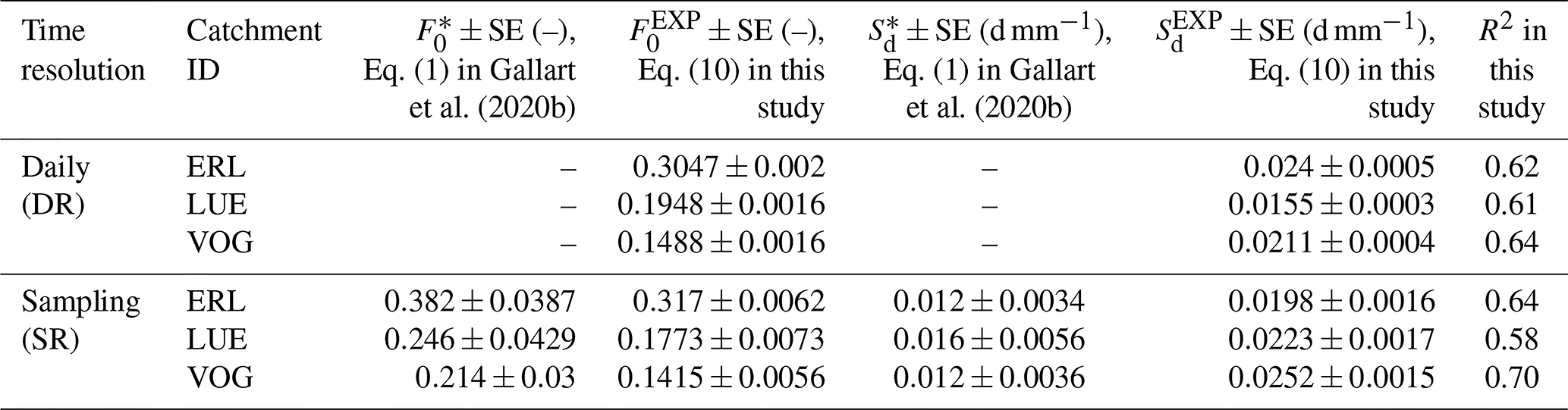
We also find that the values obtained at the SR can differ from those at the DR. For LUE, at the SR is larger than at the DR (Table 4), whereas it is the other way around for ERL. Such differences can be attributed to the different flow regimes represented by the isotope samples that influence the EC endmember estimations at each site (Table 3). Moreover, at the DR, we are calibrating the EC endmembers using Fyw and based on isotope data at the SR. To be fully consistent in terms of the temporal resolution, we theoretically need daily stream water isotope data to derive Fyw and . The influence of sampling frequency is one of the limitations of the EXPECT method, as explained in Sect. 3.3. Nevertheless, the values are consistent between the two temporal resolutions.
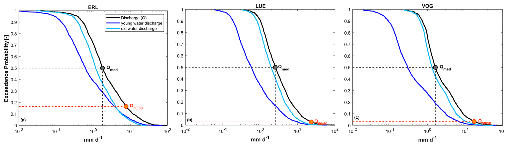
Figure 6Total flow, young flow and old flow duration curves of the (a) ERL, (b) LUE and (c) VOG catchments. indicates the median discharge value at which 50±1 % of both young and old water exists in streamflow. Qmed represents the median stream discharge.
As can be seen in Fig. 5, the values obtained with the EXPECT method form a data cloud around the idealized discharge sensitivity function of Eq. (10). Specifically, for a given discharge value, we obtain various values, which can be explained by the delayed response of old water during precipitation events: while the young water fraction is generally highest during the rising limb of the hydrograph, it decreases during the falling limb when old water reaches the stream (von Freyberg et al., 2018a, b)
3.2 An immediate application of the EXPECT method: flow duration curves of young/old water and the temporal variability in the young water fractions
Because the EXPECT method allows for the estimation of the young water fraction at up to the DR, we can determine the respective flow duration curves of young and old water discharge. Moreover, we calculate , i.e. the median discharge value at which 50±1 % of both young and old water exist in streamflow. In the ERL catchment, Fig. 6a shows that a shift from old-water-dominated streamflow towards young water-dominated streamflow occurs for discharges larger than approximately 7.7 mm d−1 (; Fig. 6a). In the LUE and VOG catchments, the streamflow contains more old water than young water for most of the flow regime (Fig. 6b, c); only on relatively few occasions, when Q exceeds (23.2 and 17.5 mm d−1, respectively), was the relative contribution of young water slightly larger than that of old water.
By comparing with the median stream discharge (Qmed), we observe that is higher than Qmed in all three study catchments (Fig. 6). This result suggests that a major proportion of old water reaches the stream more than 50 % of the time. In both the LUE and VOG catchments, is higher than in the ERL catchment, revealing that the LUE and VOG streams are dominated by old water for longer than the ERL stream. This explains why the isotope-based average young water fraction is higher in the ERL catchment than in the LUE and VOG catchments (Table 2).
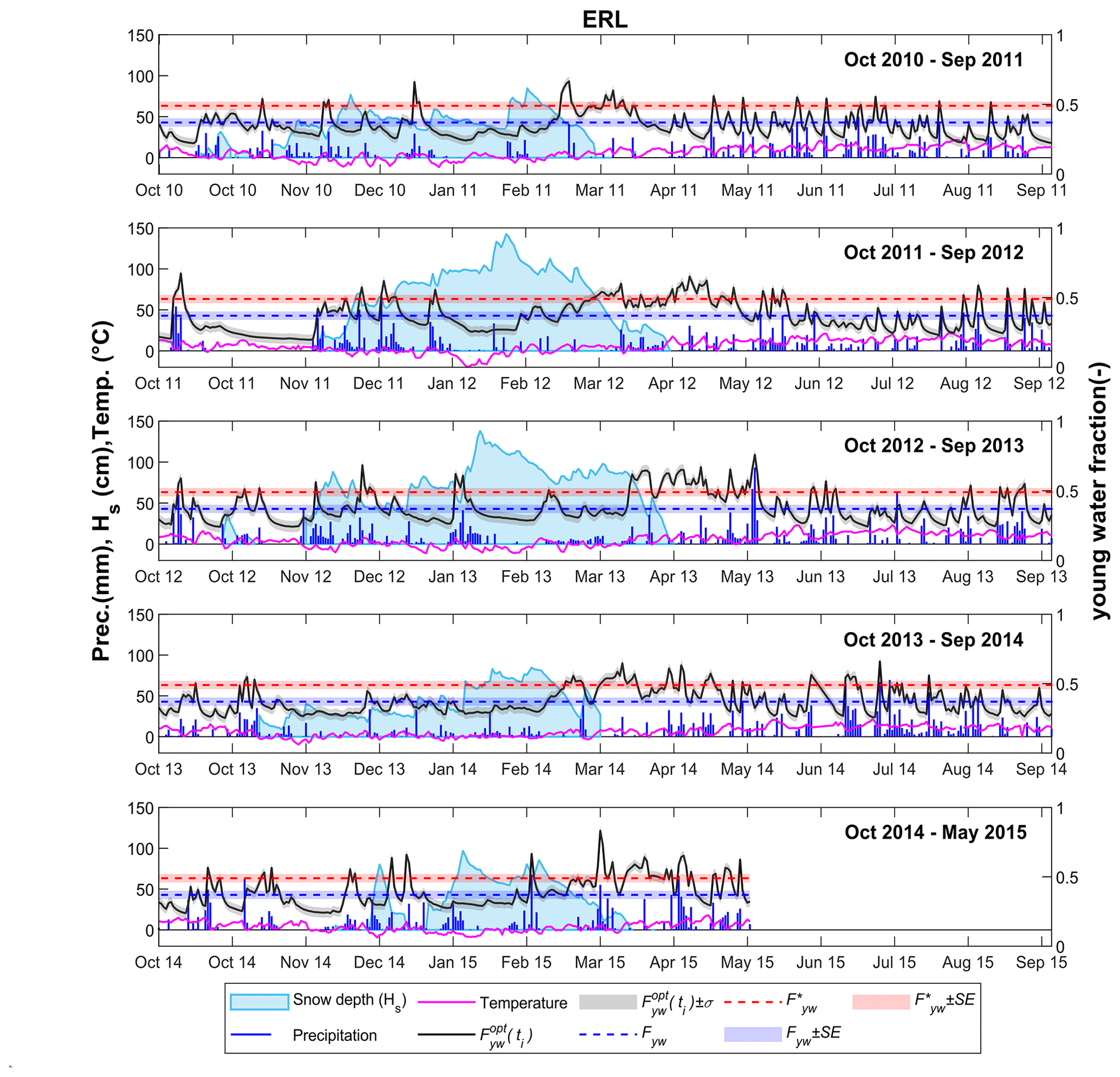
Figure 7Time series of daily precipitation, snow depth, air temperature and for the ERL catchment. Each panel reports a different hydrologic year.
With the EXPECT method, the temporal variability in can be explored in detail, e.g. by comparing time series of with those of other hydro-climatic variables (Fig. 7). Accordingly, in the following, we show a comparison between and hydro-climatic observations at the DR of the ERL catchment, as it has the most complete hydro-climatic data set (including discharge, precipitation, snow depth and temperature measurements; all data available from WSL) compared with the other two catchments. As visible from Fig. 7, daily young water fractions in the ERL catchment respond directly to precipitation events, which is further reflected by a strong positive correlation between and the daily precipitation volumes (ρSpearman=0.41, p value ≪ 0.01 considering only days with precipitation; Fig. 8). We estimate that, after a rainfall or snowmelt event, the growth rate of is on average 0.062±0.058 d−1 (to reach the local maximum next to the previous local minimum; Fig. S1 in the Supplement). On the other hand, during the recession phase, the average rate of decrease in is d−1 (to reach the local minimum next to the previous local maximum; Fig. S1). Accordingly, rapidly increases after an event (peak is reached on average after 1.98±1.25 d), while it recedes slower during no-input days (the next minimum is reached on average after 3.36±3.10 d). The largest daily young water fractions in the ERL catchment occurred during spring snowmelt (March–May), suggesting that the meltwater of the ephemeral snowpack is an important source of young water (as no relevant water ageing is observed in such a snowpack) that flows off quickly in the stream (Gentile et al., 2023). Rapid surface runoff of snowmelt can occur due to soil freezing (temperatures < 0 °C) or high soil moisture contents (temperatures > 0 °C), both of which can limit infiltration (Harrison et al., 2021; Keller et al., 2017; Fig. 7). During the periods of snow accumulation and persistent snow cover, typically from November to February, values were often as low as 0.3 and did not vary much (except during snowmelt and rain-on-snow events). Thus, streamflow in ERL was mainly composed of old water during this period, likely originating from the soil and groundwater storages.
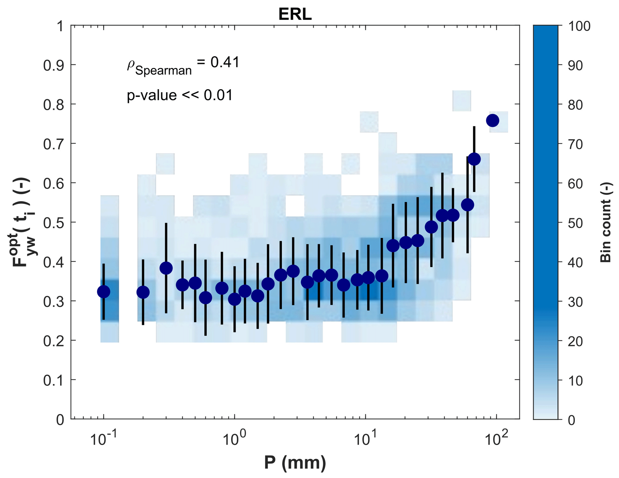
Figure 8Correlation between daily and daily precipitation when precipitation is higher than 0. Blue points indicate the median observed in the stream corresponding to different ranges of daily precipitation with error bars indicating the standard deviation. These median values are plotted against the median daily precipitation in each range. The blue colour gradient of the bins indicates the number of observations within each bin. A rapid increase in the young water fraction is observed when the daily precipitation is higher than 10 mm d−1, reflecting hydrological connectivity and the generation of rapid flow paths.
3.3 Limitations of the EXPECT method and recommendations for future applications
While the EXPECT method can offer valuable insights into the young water fraction's discharge sensitivity and its temporal variability, it is not without its limitations. The assumption that EC is a proxy for stream water age may not hold true in all hydrological systems. For example, human activities, such as mining, irrigation or wastewater inputs can alter the stream water EC in unpredictable ways. Another example involves catchments with highly soluble rocks in the aquifers (e.g. limestone or gypsum) that are susceptible to dissolution by water. It has been shown that EC can increase with Q in some karst systems due to the remobilization of circulating water in the fractured areas (Balestra et al., 2022). Therefore, the Fyw–EC relationship (Eq. 3) can be very different from that in our three study catchments, which are mainly groundwater-influenced systems. Indeed, an early study also advised that one should be mindful of EC behaviour, as it depends on the specific characteristics of each catchment (Laudon and Slaymaker, 1997). Accordingly, for future applications of the method presented in this paper, we recommend visualization of the relationship between flow-specific young water fractions and flow-specific electrical conductivities with the aim of constructing a site-specific mixing relationship, as suggested by Kirchner (2016b). It should be noted that this relationship could potentially be different from an exponential mixing model. Indeed, the use of an exponential mixing model is not proposed to be the definitive answer to the problem of choosing the right mixing model for flow partitioning into young and old water. Accordingly, if the most suitable mixing model turns out to be different from an exponential mixing model, the equations presented in this study will need to be adapted to the specific case study. However, the method's application scheme for calibrating the endmembers can still be employed. Nevertheless, in some catchments with short and sparse isotope time series, flow-specific young water fractions cannot be estimated reliably (von Freyberg et al., 2018b). The study by von Freyberg et al. (2018a) was able to estimate reliable flow-specific young water fractions for nine Swiss catchments that comprised 4- to 5-year-long isotope time series with a minimum number of 81 samples to a maximum number of 140 samples, where stream water grab samples were collected approximately fortnightly. Thus, we suggest an isotope data set with these characteristics to construct a reliable site-specific mixing model with both flow-specific EC and .
Another major limitation of the EXPECT method is its strong dependency on reliable Fyw and estimates, i.e. assumptions (ii) and (iii) in Sect. 2.2. If stream water isotope data sets are short or sparse, Fyw or can be highly uncertain and EC endmembers cannot be sufficiently constrained. Recently, Gallart et al. (2020a) revealed that unweighted and flow-weighted young water fractions were significantly lower than results with virtual (perfect) sampling when using a weekly sampling frequency. Thus, for the same catchment, we could potentially obtain different EC endmembers if stable water isotopes were sampled at higher or lower temporal resolution. Accordingly, we strongly recommend evaluating how the uncertainty in Fyw or propagates in the uncertainty in the calibrated endmembers, as described in Sect. 2.2.
For many catchments, Q and EC values are measured at a sub-hourly resolution. Thus, theoretically, the EXPECT method could provide reasonable young water fraction estimate results at these resolutions as well. However, we should consider that short-term variations in EC may not necessarily represent short-term variations in water age. For example, for a small stream in Sweden, Calles (1982) showed that diurnal variations in EC seem to be due to evapotranspiration but that the influence of gravity variations may also play a role. Moreover, a past study in a pre-alpine river in Switzerland revealed that the diurnal fluctuation in EC can be due to biogeochemical processes, such as calcite precipitation and photosynthesis (Hayashi et al., 2012). Accordingly, biological (photosynthesis and respiration) and chemical processes (carbonate equilibrium and calcite precipitation) can play a key role in controlling Ca2+ and HCO concentrations and, consequently, EC (Nimick et al., 2011; Hayashi et al., 2012). By calculating the average daily EC, and thus removing diurnal and nocturnal EC dynamics, it should better reflect variations in water age under the assumptions of the EXPECT method. Accordingly, we recommend applying the method using the daily mean of EC.
The discharge sensitivity of the young water fraction () is a useful metric that quantifies how the proportion of streamflow younger than 2–3 months changes as a catchment becomes wetter. In a past study, was obtained by fitting a sine function to the stream water isotope values, assuming an exponential relationship between the young water fraction and discharge (Gallart et al., 2020b). Most available stream water isotope data sets are characterized by a relatively low sampling frequency, which often fails to capture the entire flow regime from very low to very high discharges. This can result in highly uncertain or unrealistic estimates of the discharge sensitivity of young water fractions. Therefore, this paper aims to incorporate EC and δ18O data to develop a new method that (a) estimates young water fractions at high temporal resolution by taking advantage of continuous EC measurements and (b) better constrains the estimated discharge sensitivity.
We have designed the EXPECT method that combines a sine-wave model of the seasonal isotope cycles and an alternative EC-based hydrograph separation. Specifically, we use an exponential mixing model in which EC endmembers are calibrated using unweighted and flow-weighted young water fractions obtained from δ18O data. By considering the calibrated endmembers, daily and biweekly (sampling) young water fractions are estimated using EC measurements considered to be a proxy for the water age. The EXPECT method was tested in three small experimental catchments in Switzerland.
The application of this multi-tracer method has revealed that the optimal EC endmembers lie beyond the range of measured EC in stream water. This result reflects that streams are commonly a mixture of young and old water and that corresponding EC endmembers are difficult to obtain experimentally. The discharge sensitivities of the young water fractions obtained with the EXPECT method agree well with those obtained with the conventional approach, which uses only isotope data. However, the EXPECT method significantly reduced the standard error in the discharge sensitivity. In addition, the method allows for the estimation of young water fractions at a daily resolution, thereby providing interesting insights into short-term variations in the stream water age with changes in meteorological conditions, e.g. during snow accumulation and snowmelt. Young water fractions at a biweekly (i.e. sampling) resolution also revealed high reliability, highlighting the general applicability of this method in ungauged catchments: δ18O and EC data can both be obtained from laboratory analysis of collected water samples, while Q can be directly measured in the stream during sampling campaigns using conventional methods (e.g. the current meter method or weir method) without the presence of fixed instrumentation for measuring Q and EC.
To conclude, a recent review paper (Benettin et al., 2022) highlighted the challenge of integrating non-conservative tracers in lumped models due to a missed definition of catchment-scale chemical properties. Overall, the EC for the three study catchments was found to be an informative property that keeps track, in an integrated way, of faster (younger) and slower (older) flow paths at the catchment scale. Considering the necessary precautions regarding the use of EC, the methodology presented in this paper can be applied (with possible adaptations) to other catchments to generate new insights into transit times, hydrologic flow paths and related sources.
In order to use EC to separate the hydrograph into young and old water at a specified time ti, we may employ the two-component EC-based hydrograph separation (ECHS), built on the water (Eq. A1) and tracer (Eq. A2) mass balance:
where EC(ti) is the electrical conductivity measured in the stream at the time ti, ECyw is the young water EC endmember and ECow is the old water EC endmember. By solving the system of two equations (Eqs. A1 and A2) with two variables (Fyw(ti) and Fow(ti)), we can obtain the explicit expression of Fyw(ti):
As mentioned in Sect. 2.2, we assume ECyw < ECow. However, by performing the constrained ECHS (Sect. 2.2), in which the two endmembers (ECyw and ECow) are calibrated, the optimization algorithm finds ECyw=0, which is exactly the lower bound of the defined range [0, +∞) in which the optimization algorithm searches for the solution. This result suggests that the algorithm wants to search for the best solution below the lower bound of the specified range, thereby potentially returning a negative ECyw value. This is consistent with the negative ECyw obtained by fitting a linear model on the median EC vs. of the three study catchments (Fig. 3). Obviously, this mathematical solution is not physically acceptable, but we can investigate this result to better understand the catchment functioning. Accordingly, if we make evaluate the expression of EC(ti) starting from Eq. (A3), we find a linear decrement of EC(ti) with the increasing Fyw(ti) (Eq. A4):
By requiring a negative ECyw as the best solution, the constrained ECHS suggests that, for an exhaustive description of the catchments' behaviour, EC(ti) needs to rapidly decrease at low Fyw(ti), as shown by the red lines in Fig. A1. Nevertheless, physical reasons limit the slope (α) of this line (α ≥ −ECow); the most extreme, although still acceptable, condition (i.e. when ECyw=0 and ) is indicated by the dashed black line in Fig. A1a and b. Accordingly, to obtain a rapid decrease in EC(ti) at low Fyw(ti) and also maintain positive ECyw, it is necessary to improve the linear mixing model. As visible from Fig. A1b, the exponential mixing model described in Sect. 2.2 was suitable to describe a rapid decrease in EC(ti) at low Fyw(ti) and maintain positive ECyw.
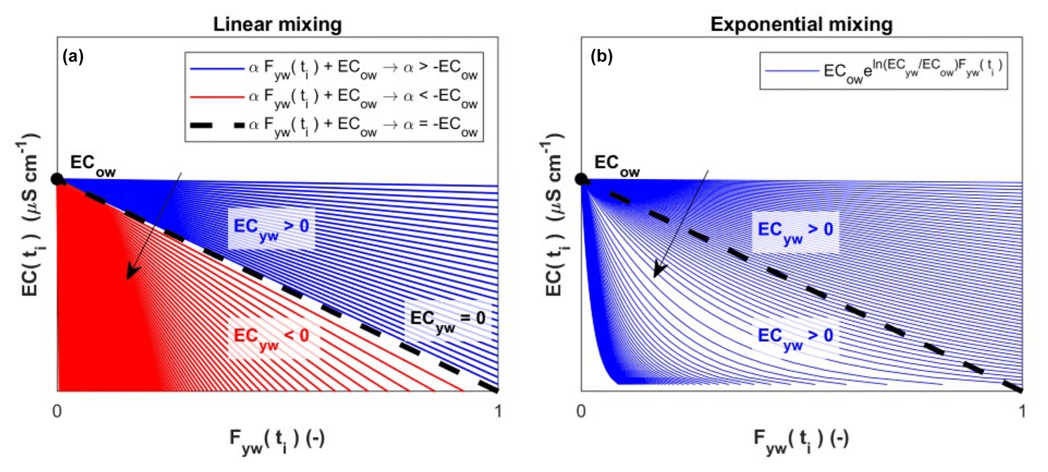
Figure A1(a) Limits of the linear decay of EC(ti) with increasing Fyw(ti). Red lines with a slope (α) lower than −ECow are not physically admitted because they imply a negative ECyw; (b) the exponential mixing overcomes this limit. Black arrows indicate the direction in which ECyw decreases.
| List of symbols. | |
| * | Indicates a flow-weighted variable |
| a | Parameter of the exponential mixing model reported in Eq. (3) |
| AP | Precipitation isotope cycle amplitude (‰) obtained via a volume-weighted robust fit of a sine |
| function to the isotopic composition of precipitation | |
| AS | Stream water isotope cycle amplitude (‰) obtained via a robust fit of a sine function to the isotopic |
| composition of stream water | |
| Stream water isotope cycle amplitude (‰) obtained via a flow-weighted robust fit of a sine function | |
| to the isotopic composition of stream water | |
| Stream water isotope cycle amplitude (‰) varying with discharge: | |
| Stream water seasonal isotope cycles amplitude (‰) obtained by fitting sinusoids separately to the | |
| isotope data collected in different discrete flow regimes, as described in Kirchner (2016b) and von | |
| Freyberg et al. (2018a) | |
| CP | Isotopic composition of precipitation (‰) |
| CS | Isotopic composition of stream water (‰) |
| DR | Daily resolution |
| EC | Electrical conductivity (µS cm−1) |
| EC(ti) | Electrical conductivity (µS cm−1) in stream water at the generic time ti |
| ECyw | Young water electrical conductivity endmember (µS cm−1) |
| EC | First-order estimate of the young water electrical conductivity endmember (µS cm−1) obtained by |
| evaluating the exponential model, fitted on the median-flow-specific EC vs. , for | |
| EC | Optimized young water electrical conductivity endmember (µS cm−1) derived from calibration |
| ECow | Old water electrical conductivity endmember (µS cm−1) |
| EC | First-order estimate of the old water electrical conductivity endmember (µS cm−1) obtained by |
| evaluating the exponential model, fitted on the median-flow-specific EC vs. , for | |
| EC | Optimized old water electrical conductivity endmember (µS cm−1) derived from calibration |
| ECHS | EC-based hydrograph separation |
| ERL | Erlenbach catchment |
| EXPECT | Two-component electrical-conductivity-based hydrograph separaTion employing an EXPonential |
| mixing model. |
| f | Frequency of the seasonal cycle (equal to once per year for a seasonal cycle) |
| Fyw | Unweighted average isotope-based young water fraction (–) obtained as |
| Unweighted average hydrograph-separation-based young water fraction (–) obtained with the | |
| exponential mixing model | |
| Flow-weighted average isotope-based young water fraction (–) obtained as | |
| Flow-weighted average hydrograph-separation-based young water fraction (–) obtained with the | |
| exponential mixing model | |
| Young water fraction (–) varying with discharge following the exponential-type equation of Gallart et | |
| al. (2020b) | |
| Fyw(ti) | Young water fraction (–) at the generic time ti |
| Fow(ti) | Old water fraction (–) at the generic time ti |
| Optimized young water fractions (–), obtained with the exponential mixing model, using the | |
| calibrated endmembers EC and EC | |
| Optimized young water fraction (-) at the generic time ti, obtained with the exponential mixing model, | |
| using the calibrated endmembers EC and EC | |
| Virtual young water fraction (–) when Q=0 in the exponential-type equation of Gallart et al. (2020b) | |
| Virtual young water fraction (–) when Q=0 obtained by fitting Eq. (6) of Gallart et al. (2020b) on | |
| vs. Q data. | |
| Young water fractions (–) estimated in discrete flow regimes as described in Kirchner (2016b) and von | |
| Freyberg et al. (2018a): | |
| HS | Hydrograph separation |
| HS | Snow depth (cm) |
| ID | Identifier |
| IHS | Isotope hydrograph separation |
| IQR | Interquartile range |
| k | Number (–) of precipitation isotope samples |
| Constant (‰) representing the vertical offset of the seasonal cycle | |
| LUE | Lümpenenbach catchment |
| n | Number (–) of Q and EC observations |
| m | Number (–) of stream water isotope samples |
| MTT | Mean transit time |
| obj | Objective function |
| Old water | Water with transit times roughly higher than 2–3 months (definition given in this paper) |
| P | Precipitation (mm) |
| P(tk) | Volume of precipitation (mm) used for the volume-weighted fit of precipitation isotopes |
| q1 | 1st quartile |
| q2 | 2nd quartile |
| q3 | 3rd quartile |
| Q | Discharge (mm d−1) |
| Qmed | Median stream discharge (mm d−1) |
| Q(ti) | Discharge at the time ti (mm d−1) |
| Q(tj) | Discharge at the time tj (mm d−1) |
| Median discharge (mm d−1) at which 50±1 % of both young and old water exists in streamflow | |
| Young water | Water with transit times roughly lower than 2–3 months (definition given in this paper) |
| Discharge sensitivity of young water fraction (d mm−1) obtained with the method of Gallart et al. (2020b) | |
| Discharge sensitivity of young water fraction (d mm−1) obtained by fitting Eq. (6) of Gallart et al. (2020b) | |
| on vs. Q data | |
| SE | Standard error |
| SR | Sampling resolution |
| ti | Generic time in which Q and EC are measured |
| tj | Generic time in which a stream water isotope sample is collected |
| tk | Generic time in which a precipitation isotope sample is collected |
| VOG | Vogelbach catchment |
| δ2H | Isotope content (‰) considering deuterium |
| δ18O | Isotope content (‰) considering oxygen-18 |
| δ18Op | Isotope content of precipitation (‰) considering oxygen-18 |
| δ18OP(tk) | Isotope content of precipitation (‰) at time tk considering oxygen-18 |
| δ18OS | Isotope content of stream water (‰) considering oxygen-18 |
| δ18OS(ti) | Isotope content of stream water (‰) at time ti considering oxygen-18 |
| Phase of the seasonal cycle (rad) | |
| σ | Standard deviation |
| ρSpearman | Spearman correlation coefficient |
Time series of δ18O in streamflow and precipitation for the ERL, LUE and VOG catchments are available from Zenodo at https://doi.org/10.5281/zenodo.4057967 (Staudinger et al., 2020b) and are presented and described in Staudinger et al. (2020a). Daily discharge and electrical conductivity data for the ERL, LUE and VOG catchments are available from the Swiss Federal Institute for Forest, Snow and Landscape research (WSL) data portal: https://doi.org/10.16904/envidat.380 (Stähli, 2018). The shapefiles (.shp) for the ERL, LUE and VOG catchments are available from https://doi.org/10.5281/zenodo.4057967 (Staudinger et al., 2020b).
The supplement related to this article is available online at: https://doi.org/10.5194/hess-28-1915-2024-supplement.
AG, JvF and SF identified the research gap, designed the EXPECT method and prepared the paper. AG implemented the EXPECT method in a MATLAB code with support from DG and DC. All authors revised the manuscript and approved the submitted version.
The contact author has declared that none of the authors has any competing interests.
Publisher's note: Copernicus Publications remains neutral with regard to jurisdictional claims made in the text, published maps, institutional affiliations, or any other geographical representation in this paper. While Copernicus Publications makes every effort to include appropriate place names, the final responsibility lies with the authors.
This work was supported by the PRIN MIUR 2017SL7ABC_005 WATZON Project, by the PRIN 2022 202295PFKP SUNSET Project and by Funding 2021 Fondazione CRT. Jana von Freyberg was supported by the Swiss National Science Foundation (SNSF; grant no. PR00P2_185931). The results of this study have been discussed within the COST Action WATSON, CA19120, supported by COST (European Cooperation in Science and Technology).
This publication is part of the NODES project, which has received funding from the MUR – M4C2 1.5 of PNRR (grant no. ECS00000036).
This paper was edited by Natalie Orlowski and reviewed by two anonymous referees.
Balestra, V., Fiorucci, A., and Vigna, B.: Study of the Trends of Chemical–Physical Parameters in Different Karst Aquifers: Some Examples from Italian Alps, Water, 14, 441, hhttps://doi.org/10.3390/w14030441, 2022.
Benettin, P., Bailey, S. W., Campbell, J. L., Green, M. B., Rinaldo, A., Likens, G. E., McGuire, K. J., and Botter, G.: Linking water age and solute dynamics in streamflow at the Hubbard Brook Experimental Forest, NH, USA, Water Resour. Res., 51, 9256–9272, https://doi.org/10.1002/2015WR017552, 2015.
Benettin, P., Bailey, S. W., Rinaldo, A., Likens, G. E., McGuire, K. J., and Botter, G.: Young runoff fractions control streamwater age and solute concentration dynamics, Hydrol. Process., 31, 2982–2986, https://doi.org/10.1002/hyp.11243, 2017.
Benettin, P., Rodriguez, N. B., Sprenger, M., Kim, M., Klaus, J., Harman, C. J., van der Velde, Y., Hrachowitz, M., Botter, G., McGuire, K. J., Kirchner, J. W., Rinaldo, A., and McDonnell, J. J.: Transit Time Estimation in Catchments: Recent Developments and Future Directions, Water Resour. Res., 58, e2022WR033096, https://doi.org/10.1029/2022WR033096, 2022.
Bonacci, O. and Roje-Bonacci, T.: Water temperature and electrical conductivity as an indicator of karst aquifer: the case of Jadro Spring (Croatia), Carbon. Evaporit., 38, 55, https://doi.org/10.1007/s13146-023-00881-x, 2023.
Calles, U. M.: Diurnal Variations in Electrical Conductivity of Water in a Small Stream, Hydrol. Res., 13, 157–164, https://doi.org/10.2166/nh.1982.0013, 1982.
Camacho Suarez, V. V., Saraiva Okello, A. M. L., Wenninger, J. W., and Uhlenbrook, S.: Understanding runoff processes in a semi-arid environment through isotope and hydrochemical hydrograph separations, Hydrol. Earth Syst. Sci., 19, 4183–4199, https://doi.org/10.5194/hess-19-4183-2015, 2015.
Cano-Paoli, K., Chiogna, G., and Bellin, A.: Convenient use of electrical conductivity measurements to investigate hydrological processes in Alpine headwaters, Sci. Total Environ., 685, 37–49, https://doi.org/10.1016/j.scitotenv.2019.05.166, 2019.
Cey, E. E., Rudolph, D. L., Parkin, G. W., and Aravena, R.: Quantifying groundwater discharge to a small perennial stream in southern Ontario, Canada, J. Hydrol., 210, 21–37, https://doi.org/10.1016/S0022-1694(98)00172-3, 1998.
Dansgaard, W.: Stable isotopes in precipitation, Tellus, 16, 436–468, https://doi.org/10.3402/tellusa.v16i4.8993, 1964.
Gallart, F., Valiente, M., Llorens, P., Cayuela, C., Sprenger, M., and Latron, J.: Investigating young water fractions in a small Mediterranean mountain catchment: Both precipitation forcing and sampling frequency matter, Hydrol. Process., 34, 3618–3634, https://doi.org/10.1002/hyp.13806, 2020a.
Gallart, F., von Freyberg, J., Valiente, M., Kirchner, J. W., Llorens, P., and Latron, J.: Technical note: An improved discharge sensitivity metric for young water fractions, Hydrol. Earth Syst. Sci., 24, 1101–1107, https://doi.org/10.5194/hess-24-1101-2020, 2020b.
Gentile, A., Canone, D., Ceperley, N., Gisolo, D., Previati, M., Zuecco, G., Schaefli, B., and Ferraris, S.: Towards a conceptualization of the hydrological processes behind changes of young water fraction with elevation: a focus on mountainous alpine catchments, Hydrol. Earth Syst. Sci., 27, 2301–2323, https://doi.org/10.5194/hess-27-2301-2023, 2023.
Harrison, H. N., Hammond, J. C., Kampf, S., and Kiewiet, L.: On the hydrological difference between catchments above and below the intermittent-persistent snow transition, Hydrol. Process., 35, e14411, https://doi.org/10.1002/hyp.14411, 2021.
Hayashi, M., Vogt, T., Mächler, L., and Schirmer, M.: Diurnal fluctuations of electrical conductivity in a pre-alpine river: Effects of photosynthesis and groundwater exchange, J. Hydrol., 450–451, 93–104, https://doi.org/10.1016/j.jhydrol.2012.05.020, 2012.
Hooper, R. P.: Diagnostic tools for mixing models of stream water chemistry, Water Resour. Res., 39, 1055, https://doi.org/10.1029/2002WR001528, 2003.
Keller, D. E., Fischer, A. M., Liniger, M. A., Appenzeller, C., and Knutti, R.: Testing a weather generator for downscaling climate change projections over Switzerland, Int. J. Climatol., 37, 928–942, https://doi.org/10.1002/joc.4750, 2017.
Kendall, C. and McDonnell, J. J.: Isotope Tracers in Catchment Hydrology, in: 1st Edn., Elsevier, 839 pp., ISBN 978-0-444-81546-0, 1998.
Kiewiet, L., van Meerveld, I., Stähli, M., and Seibert, J.: Do stream water solute concentrations reflect when connectivity occurs in a small, pre-Alpine headwater catchment?, Hydrol. Earth Syst. Sci., 24, 3381–3398, https://doi.org/10.5194/hess-24-3381-2020, 2020.
Kirchner, J. W.: Aggregation in environmental systems – Part 1: Seasonal tracer cycles quantify young water fractions, but not mean transit times, in spatially heterogeneous catchments, Hydrol. Earth Syst. Sci., 20, 279–297, https://doi.org/10.5194/hess-20-279-2016, 2016a.
Kirchner, J. W.: Aggregation in environmental systems – Part 2: Catchment mean transit times and young water fractions under hydrologic nonstationarity, Hydrol. Earth Syst. Sci., 20, 299–328, https://doi.org/10.5194/hess-20-299-2016, 2016b.
Klaus, J. and McDonnell, J. J.: Hydrograph separation using stable isotopes: Review and evaluation, J. Hydrol., 505, 47–64, https://doi.org/10.1016/j.jhydrol.2013.09.006, 2013.
Laudon, H. and Slaymaker, O.: Hydrograph separation using stable isotopes, silica and electrical conductivity: an alpine example, J. Hydrol., 201, 82–101, https://doi.org/10.1016/S0022-1694(97)00030-9, 1997.
Lazo, P. X., Mosquera, G. M., Cárdenas, I., Segura, C., and Crespo, P.: Flow partitioning modelling using high-resolution electrical conductivity data during variable flow conditions in a tropical montane catchment, J. Hydrol., 617, 128898, https://doi.org/10.1016/j.jhydrol.2022.128898, 2023.
McGuire, K. J. and McDonnell, J. J.: A review and evaluation of catchment transit time modeling, J. Hydrol., 330, 543–563, https://doi.org/10.1016/j.jhydrol.2006.04.020, 2006.
Meriano, M., Howard, K. W. F., and Eyles, N.: The role of midsummer urban aquifer recharge in stormflow generation using isotopic and chemical hydrograph separation techniques, J. Hydrol., 396, 82–93, https://doi.org/10.1016/j.jhydrol.2010.10.041, 2011.
Monteith, D. T., Henrys, P. A., Hruška, J., de Wit, H. A., Krám, P., Moldan, F., Posch, M., Räike, A., Stoddard, J. L., Shilland, E. M., Pereira, M. G., and Evans, C. D.: Long-term rise in riverine dissolved organic carbon concentration is predicted by electrolyte solubility theory, Sci. Adv., 9, eade3491, https://doi.org/10.1126/sciadv.ade3491, 2023.
Mosquera, G. M., Segura, C., Vaché, K. B., Windhorst, D., Breuer, L., and Crespo, P.: Insights into the water mean transit time in a high-elevation tropical ecosystem, Hydrol. Earth Syst. Sci., 20, 2987–3004, https://doi.org/10.5194/hess-20-2987-2016, 2016.
Mosquera, G. M., Segura, C., and Crespo, P.: Flow Partitioning Modelling Using High-Resolution Isotopic and Electrical Conductivity Data, Water, 10, 904, https://doi.org/10.3390/w10070904, 2018.
Nimick, D. A., Gammons, C. H., and Parker, S. R.: Diel biogeochemical processes and their effect on the aqueous chemistry of streams: A review, Chem. Geol., 283, 3–17, https://doi.org/10.1016/j.chemgeo.2010.08.017, 2011.
Pellerin, B. A., Wollheim, W. M., Feng, X., and Vörösmarty, C. J.: The application of electrical conductivity as a tracer for hydrograph separation in urban catchments, Hydrol. Process., 22, 1810–1818, https://doi.org/10.1002/hyp.6786, 2008.
Penna, D., Engel, M., Mao, L., Dell'Agnese, A., Bertoldi, G., and Comiti, F.: Tracer-based analysis of spatial and temporal variations of water sources in a glacierized catchment, Hydrol. Earth Syst. Sci., 18, 5271–5288, https://doi.org/10.5194/hess-18-5271-2014, 2014.
Penna, D., Engel, M., Bertoldi, G., and Comiti, F.: Towards a tracer-based conceptualization of meltwater dynamics and streamflow response in a glacierized catchment, Hydrol. Earth Syst. Sci., 21, 23–41, https://doi.org/10.5194/hess-21-23-2017, 2017.
Riazi, Z., Western, A. W., and Bende-Michl, U.: Modelling electrical conductivity variation using a travel time distribution approach in the Duck River catchment, Australia, Hydrol. Process., 36, e14721, https://doi.org/10.1002/hyp.14721, 2022.
Schmidt, C., Musolff, A., Trauth, N., Vieweg, M., and Fleckenstein, J. H.: Transient analysis of fluctuations of electrical conductivity as tracer in the stream bed, Hydrol. Earth Syst. Sci., 16, 3689–3697, https://doi.org/10.5194/hess-16-3689-2012, 2012.
Stähli, M.: Longterm hydrological observatory Alptal (central Switzerland), EnviDat [data set], https://doi.org/10.16904/envidat.380, 2018.
Stähli, M., Seibert, J., Kirchner, J. W., von Freyberg, J., and van Meerveld, I.: Hydrological trends and the evolution of catchment research in the Alptal valley, central Switzerland, Hydrol. Process., 35, e14113, https://doi.org/10.1002/hyp.14113, 2021.
Staudinger, M., Stoelzle, M., Seeger, S., Seibert, J., Weiler, M., and Stahl, K.: Catchment water storage variation with elevation, Hydrol. Process., 31, 2000–2015, https://doi.org/10.1002/hyp.11158, 2017.
Staudinger, M., Seeger, S., Herbstritt, B., Stoelzle, M., Seibert, J., Stahl, K., and Weiler, M.: The CH-IRP data set: a decade of fortnightly data on δ2H and δ18O in streamflow and precipitation in Switzerland, Earth Syst. Sci. Data, 12, 3057–3066, https://doi.org/10.5194/essd-12-3057-2020, 2020a.
Staudinger, M., Seeger, S., Herbstritt, B., Stoelzle, M., Seibert, J., Stahl, K., and Weiler, M.: The CH-IRP data set: fortnightly data of δ2H and δ18O in streamflow and precipitation in Switzerland (Version 2), Zenodo [data set], https://doi.org/10.5281/zenodo.4057967, 2020b.
von Freyberg, J., Allen, S. T., Seeger, S., Weiler, M., and Kirchner, J. W.: Sensitivity of young water fractions to hydro-climatic forcing and landscape properties across 22 Swiss catchments, Hydrol. Earth Syst. Sci., 22, 3841–3861, https://doi.org/10.5194/hess-22-3841-2018, 2018a.
von Freyberg, J., Studer, B., Rinderer, M., and Kirchner, J. W.: Studying catchment storm response using event- and pre-event-water volumes as fractions of precipitation rather than discharge, Hydrol. Earth Syst. Sci., 22, 5847–5865, https://doi.org/10.5194/hess-22-5847-2018, 2018b.
Wang, L., von Freyberg, J., van Meerveld, I., Seibert, J., and Kirchner, J. W.: What is the best time to take stream isotope samples for event-based model calibration?, J. Hydrol., 577, 123950, https://doi.org/10.1016/j.jhydrol.2019.123950, 2019.
Xia, C., Zuecco, G., Chen, K., Liu, L., Zhang, Z., and Luo, J.: The estimation of young water fraction based on isotopic signals: challenges and recommendations, Front. Ecol. Evol., 11, 1114259, https://doi.org/10.3389/fevo.2023.1114259, 2023.
Zuecco, G., Penna, D., and Borga, M.: Runoff generation in mountain catchments: long-term hydrological monitoring in the Rio Vauz Catchment, Italy, Cuad. Investig. Geográfica, 44, 397–428, https://doi.org/10.18172/cig.3327, 2018.