A coupled atmospheric–hydrologic modeling system with variable grid sizes for rainfall–runoff simulation in semi-humid and semi-arid watersheds: how does the coupling scale affects the results?

The coupled atmospheric–hydrologic modeling system is an effective way to improve the accuracy of rainfall–runoff modeling and extend the lead time in real-time flood forecasting. The aim of this study is to explore the appropriate coupling scale of the coupled atmospheric–hydrologic modeling system, which is established by the Weather Research and Forecasting (WRF) model and the gridded Hebei model with three different sizes (1 km×1 km, 3 km×3 km and 9 km×9 km). The Hebei model is a conceptual rainfall–runoff model designed to describe a mixed runoff generation mechanism, including both storage excess and infiltration excess, in the semi-humid and semi-dry area of northern China. The soil moisture storage capacity and infiltration capacity of different grids in the gridded Hebei model are obtained and dispersed using the topographic index. The lumped Hebei model is also used to establish the lumped atmospheric–hydrologic coupled system as a reference system. Four 24 h storm events occurring at two small- and medium-scale sub-watersheds in northern China are selected as case studies. Contrastive analyses of the flood process simulations from the gridded and lumped systems are carried out. The results show that the flood simulation results may not always be improved with higher-dimension precision and more complicated system, and the grid size selection has a strong relationship with the rainfall evenness. For the storm events with uniform spatial distribution, the coupling scale has less impact on flood simulation results, and the lumped system also performs well. For the storm events with uneven spatiotemporal distribution, the corrected rainfall can improve the simulation results significantly, and higher resolution leads to better flood process simulation. The results can help to establish the appropriate coupled atmospheric–hydrologic modeling system to improve the flood forecasting accuracy.

1 Introduction

Compared to the traditional flood forecast models that take gauge precipitation as inputs, the coupling of a mesoscale numerical weather prediction (NWP) model with a hydrological model has been proven to be an effective way to improve the accuracy of rainfall–runoff modeling and extend the lead time in real-time flood forecasting (Wu et al., 2014; Wan and Xu, 2011). The atmospheric–hydrologic coupled system has become the current world technology frontier for flood forecasting, and correlation studies have received extensive attention (Benoit et al., 2000; Tian et al., 2019). Given the multiscale nature of watershed hydrologic models and rainfall data output by numerical atmospheric models, one key to obtaining accurate simulations results is the establishment of a suitable atmospheric–hydrologic coupled system.

Most atmospheric–hydrologic coupling studies tend to use lumped or distributed hydrological models (constructed in research watersheds) to run atmospheric models based on hydrological model requirements by inputting meteorological information such as rainfall (Wagner et al., 2016). Liu et al. (2015) simulated the floods by a lumped hydrological model integrated with the Weather Research And Forecasting (WRF) model at a 10 km scale at a small catchment (135.2 km²). Rogelis et al. (2018) focused on comparison of streamflows obtained from three different lumped hydrological models driven by WRF precipitation forecast at the Tunjuelo River basin (380 km²). The spatial resolution of 1.67 km was set for finest domain in the WRF model. Li et al. (2017) extended the flood forecasting lead time in the Liujiang River basin (58 270 km²) by WRF precipitation forecast with a distributed hydrological model. The WRF precipitation forecast with the resolution being 20 km × 20 km was downscaled to 200 m × 200 m, which was suited for the resolution of the hydrological model. However, most studies have no consideration for the spatial-scale matching issue between atmospheric and hydrological models, which has significant impact on the flood forecast accuracy.

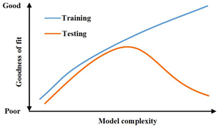
Model complexity is another impact factor that must be considered during model construction. When investigating the complexity of data-driven models, Myung et al. (2009) found that the relationship between model complexity and error can be described as in Fig. 1. It is outlined that model selection and construction should not solely be based on the goodness of fit but must also consider the model complexity (whether the model's description of observed data is achieved in the simplest possible manner). This is because a highly complex model can provide a good fit without necessarily bearing any interpretable relationship with the underlying process. It is shown that model selection based solely on the fit to observed data will result in the choice of an unnecessarily complex model that overfits the data and, thus, generalizes poorly (Myung, 2000).

Figure 1 Relationship between the model complexity and the goodness of fit of a data-driven model.

This could also be true when dealing with the coupled atmospheric–hydrologic systems. Although the models in the coupled system are physically based with deterministic structures and parameters, the complexity is to a great extent decided by choosing an appropriate spatial scale (grid size) for coupling (Verbunt et al., 2006; Hostache et al., 2011; Rogelis and Werner, 2018). A smaller coupling scale between the atmospheric and the hydrologic models helps utilize higher-resolution rainfall information, but a higher grid resolution results in a greater computational load, leading in turn to greater cumulative errors in the simulated discharge at the watershed outlet. On the other hand, a larger coupling scale allows a smaller computational load, but the accuracy of the rainfall information decreases such that the final simulation results may be subject to larger errors. Therefore, finding the underlying law of how the performance of the coupled atmospheric–hydrologic system is impacted by the coupling scale is of great importance in enhancing the accuracy of rainfall–runoff simulation. Within this scope, important issues that should be addressed in depth include how to effectively use the high-resolution rainfall information provided by atmospheric models, how to select a suitable spatial scale for constructing a coupled atmospheric–hydrologic system, and how to make tradeoffs between the computational efficiency and accuracy. Moreover, to date, the spatial scale of atmospheric–hydrologic coupling has not yet been investigated with respect to different rainfall processes.

In this study, a coupled atmospheric–hydrologic system with variable grid scales is firstly developed based on the construction of a gridded hydrologic model in combination with a mesoscale NWP model to provide rainfall driving data at different resolutions; this allows the atmospheric–hydrologic coupling at different spatial scales. The most recently developed mesoscale NWP model, i.e., the Weather Research & Forecasting (WRF) model, is adopted to provide the downscaled rainfall information and the Hebei model (Tian et al., 2019), a conceptual model with mixed runoff generation mechanisms of both saturation-excess and infiltration-excess, is used to construct the gridded hydrologic model. Three different coupling scales are considered in this study, which is 1 km×1 km, 3 km×3 km, and 9 km×9 km. Next, the coupled atmospheric–hydrologic system with different spatial scales to reflect the degree of model complexity, is applied to four storm events in semi-humid and semi-arid watersheds of northern China. The storm events are characterized by different representatives of the rainfall distribution evenness in space and time. The performance of the coupled system in different degree of complexity (i.e., with different coupling scale or grid size) is fully investigated with regard to different storm events, and the relationship between the rainfall evenness and the selection of the most appropriate coupling scale is further discussed.

Figure 2 Location map of the two study sub-watersheds.

Figure 3 Topographic map of the two study sub-watersheds with the locations of rain and flow gauge stations.

2 Data sources

2.1 Study site

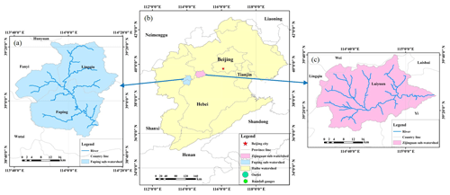
In this study, two mountainous sub-watersheds of the Daqing River basin (Fuping of the south branch and Zijingguan of the north branch) are chosen as the study area (Figs. 2 and 3). The Fuping sub-watershed has a total area of 2219 km² and is located in the upper reaches of the Shahe River, a south branch of the Daqing River. The Zijingguan sub-watershed has a total area of 1760 km² and is located in the upper reaches of the Juma River, a north branch of the Daqing River. The two sub-watersheds are the most concentrated and typical cinnamon regions. The land use mainly includes grassland, farmland, and forestland. The soil erosion is severe. Due to the dry soil conditions and the groundwater overexploitation, the river has extensive seepage during the storm season. More information about the two sub-watersheds is shown in Table 1. The study area embodies the representative rainfall–runoff characteristics of the sub-humid and sub-arid area in northern China. Rainfall in northern China is characterized by summer storms with short durations and large intensities, which are likely to result in severe flood disasters, especially in mountainous areas like Fuping and Zijingguan.

Table 1 The characteristics of the two sub-watersheds.

Figure 4 Rainfall–runoff processes of the four 24 h storm events.

2.2 Storm events

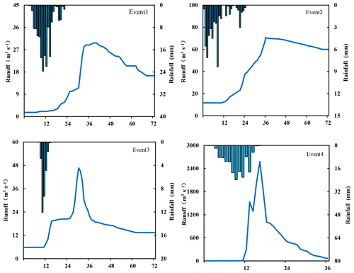
Based on the analyses of the historical floods in the study area, four representative 24 h duration storm events with relatively high flow peaks (Fig. 4) are selected and used to test the performance of the coupled atmospheric–hydrologic system for rainfall–runoff modeling. The start and end times together with the 24 h cumulative rainfall amounts and the peak discharges are listed in Table 2. Among the four events, three occur in Fuping sub-watershed and one occurs in Zijingguan sub-watershed. Before the establishment of the coupled atmospheric–hydrologic system, quality controls of the observational rainfall–runoff data are carried out. Rainfall observations from the rain gauges are verified by the weather radar, and interpolations are done to guarantee the continuity of the flow observations (Liu et al., 2018).

Table 2 Four 24 h storm events selected from the study site.

The coefficient of variation C_v is used as an indicator to verify the representativeness of the selected storm events and to characterize their temporal and spatial distributions. With regard to the spatial distribution, the coefficient reflects the variations in the 24 h cumulative rainfall among different rainfall stations across the watershed. As for the temporal distribution, it shows the variations in the average areal rainfall at different time steps during the whole storm event. The coefficient of variation C_v can thus be calculated as (Yue et al., 2014; Jha et al., 2015; Tian et al., 2017a, b)

$$\begin{array}{}\text{(1)}& C_{\mathrm{v}}=\sqrt{{\displaystyle \frac{\sum _{i=\mathrm{1}}^n{\left(\frac{x_i}{\stackrel{\mathrm{‾}}{x}}-\mathrm{1}\right)}^{\mathrm{2}}}{n}}}.\end{array}$$

For spatial distribution calculations, x_i is the 24 h cumulative rainfall at a certain rainfall station i, $\stackrel{\mathrm{‾}}{x}$ represents the average cumulative rainfall of all stations, and n refers to the number of rainfall stations in the sub-watershed. For temporal distribution calculations, x_i is the areal rainfall at the ith time step, $\stackrel{\mathrm{‾}}{x}$ is the average of the areal rainfall of all time steps, and n refers to total time steps the rainfall lasts for, which is 24 h in this study. The calculated spatial and temporal values for the four selected events can be found in Table 3. The smaller the value of C_v is, the more even the rainfall distribution is in space or time. According to Table 3, the ranking of the distribution evenness of rainfall in space is event 2 > event 1 > event 4 > event 3, and that in time is event 1 > event 2 > event 4 > event 3. Event 1 has relatively even rainfall in both space and time, and the rainfall of event 2 is evenly distributed in space but unevenly distributed in time. Both event 3 and event 4 have unevenly distributed rainfall in space and time, while event 4, which can be noted with much larger C_v values and higher cumulative rainfall, is considered to be an extreme case. The storm happened in a very short period of time and in a very concentrated area with high rainfall intensity.

Table 3 C_v values for the four storm events.

3 Experimental design with WRF and the grid-based hydrological model

3.1 Atmospheric modeling

3.1.1 WRF model setup

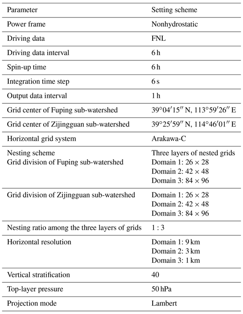
The WRF model with a variety of physical and numerical options has widely been used for numerical rainfall prediction in the catchment scale (Liu et al., 2012; Cassola et al., 2015; Tian et al., 2017b). In this study, three nested domains are adopted, centered over the Fuping sub-watershed (at 39^∘04^′15^′′ N, 113^∘59^′26^′′ E) or the Zijingguan sub-watershed (39^∘25^′59^′′ N, 114^∘46^′01^′′ E). The two sub-watersheds are totally covered by the innermost domain, with the interaction between the parent and child domain being allowed. The horizontal grid spacing is set to 1, 3, and 9 km from the innermost to the outermost domain, which is consistent with the resolution of the hydrological model and allows easy operation during coupling (Tian et al., 2017a). The NCEP/NCAR final operational global analysis (FNL) data with spatial resolution of 1^∘ × 1^∘ and temporal resolution of 1 h are used to provide the lateral and boundary conditions of the WRF model (C. C. Wang et al., 2013; H. Wang et al., 2013). In order to eliminate the discrepancy of the initial and boundary conditions with the driven data, another outermost domain is set beyond the WRF three nested domains to downscale the FNL data to a spatial resolution of 27 km. The integration time step of the model is set to 6 s, and the output data interval is set to 1 h (Hong and Lee, 2009). Forty layers are considered in the three nested domains, with a top-layer pressure of 50 hPa. The projection method is chosen to be Lambert, which has good applicability in the midlatitude regions. The other basic settings of the WRF model adopted in this study can be found in Table 4.

Table 4 Basic settings of the WRF model for the two sub-watersheds.

3.1.2 Physical parameterizations

The WRF rainfall simulation is sensitive to the selection and the combination of its physical parameterizations (Di et al., 2015). In this study, the well-performing and extensively used parameterizations in northern China were chosen (Miao et al., 2011; Di et al., 2015; Tian et al., 2017a), which include two microphysics parameterizations, i.e., Purdue-Lin (Lin) (Lin et al., 1983) and WRF Single-Moment 6 (WSM6) (Hong et al., 2006); two cumulus parameterizations, i.e., Kain–Fritsch (KF) (Kain, 2004) and Grell–Devenyi (GD) (Grell and Freitas, 2014); and two PBL (planetary boundary layer) parameterizations, i.e., Mellor–Yamada–Janjic (MYJ) (Hong et al., 2006) and Yonsei University (YSU) (Janjić, 1994). Besides, Rapid Radiative Transfer Model (RRTM) and Dudhia (Evans et al., 2012) usually cooperate well as the long- and shortwave radiation parameterizations, and Noah is chosen to be the land surface model (Chen et al., 2014). The most suitable physical parameterizations resulting the best rainfall simulations (Tian et al., 2017a) are used for each of the four storm events, as shown in Table 5. It should be clarified that the comparison of different coupling scales is carried out for each of storm event under the same model parameterizations (MPs) and thus using different MPs for different events will not cause difficulties in analyzing the final results.

Table 5 Physical parameterizations adopted for the selected storm events.

3.2 Hydrologic modeling

3.2.1 Construction of a grid-based hydrologic model

A mesoscale NWP model can produce downscaled rainfall data with different horizontal resolutions through the multilayer nested grids. In order to use the spatial information of the WRF rainfall output data, a loosely structured hydrological model is constructed in each of the two sub-watersheds. The sub-watersheds are firstly divided into grids, based on which a rainfall–runoff model is established on each grid cell to calculate the runoff generation and concentration within the grid cell. After that, a spatially distributed river network model is used to calculate the confluence of the river flow from the grids to obtain the total discharge at the outlet of the watershed. As the scale of grid-based hydrologic models is dependent on the grid size, it is possible to conduct the grid division of the watershed according to the horizontal resolution of the WRF output rainfall data.

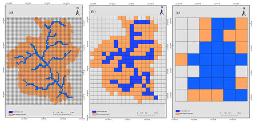
Figure 5 DEM grids for the Fuping sub-watershed with channel and non-channel cells: (a) 1 km×1 km grids, (b) 3 km×3 km grids, and (c) 9 km×9 km grids.

Figure 6 DEM grids for the Zijingguan sub-watershed with channel and non-channel cells: (a) 1 km×1 km grids, (b) 3 km×3 km grids, and (c) 9 km×9 km grids.

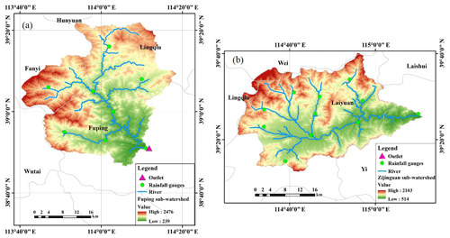
In this study, the 30 m digital elevation model (DEM) provided by Geospatial Data Cloud (http://www.gscloud.cn/, last access: 30 January 2019) assists in establishing the grid-based hydrologic model. Based on the DEMs of the two sub-watersheds and the GIS spatial analysis tools, the flow direction of each grid cell is determined, the river network is generated, and the computing orders of the grids are then obtained. Considering the horizontal resolution of the WRF model in this study is set to be 1, 3, and 9 km from the innermost to the outermost domain, the two sub-watersheds, Fuping and Zijingguan, are divided into grids with the same three resolutions. The divided 1 km×1 km, 3 km×3 km, and 9 km×9 km grids of the two sub-watersheds with a distinction between channel and non-channel cells are shown in Figs. 5 and 6.

Figure 7 Main structure of the Hebei rainfall–runoff model built on each grid cell.

3.2.2 Runoff generation and water exchange processes

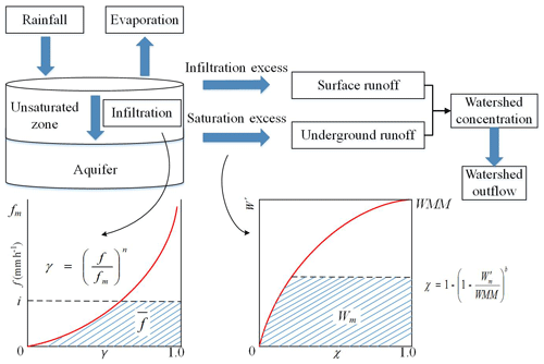
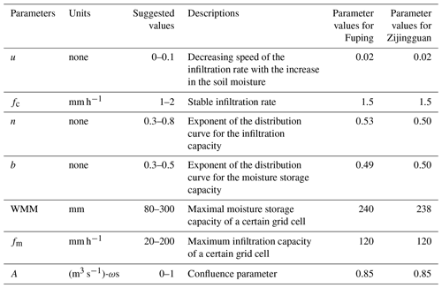
In this study, a conceptual rainfall–runoff model, named Hebei model, is built on each grid cell of the two sub-watersheds. The Hebei model is specially developed for rainfall–runoff modeling in the semi-humid and semi-dry area of northern China and has widely been applied in Hebei Province by considering both infiltration-excess and saturation-excess mechanisms of the runoff generation (Tian et al., 2019). Due to the perennial water shortage and groundwater overexploitation, both storage excess and infiltration excess are found in the study area with extensive seepage along the river channel during the storm season. The obvious advantage of the Hebei model is the consideration of both storage-excess and infiltration-excess mechanisms for rainfall–runoff generation. The model is easily applied and can be used in other semi-humid and semi-arid watersheds. In the Hebei model, the description for the storage excess part is the same as that in the Xin'anjiang model (Zhao, 1992). On the other hand, the infiltration capacity across the watershed is described by a distribution curve described below, and the Horton model is applied to calculate the seepage along the river channel during the river routing (Horton, 1933). The structure of the Hebei rainfall–runoff model is shown in Fig. 7 and calibrated parameters are listed in Table 6. γ is the proportion of the area with the infiltration capability within a certain value, χ is the proportion of no runoff generation area to entire basin area, W^′ is the storage capacity of the point in the basin, and WMM is the storage capacity of the maximum point in the basin. The surface runoff is generated when the rainfall intensity exceeds the infiltration capacity, and when the infiltrated water volume matches the soil's water shortage capacity, the surplus water generates the groundwater runoff. The total flow at the watershed outlet is composed of both the surface and the underground runoff.

Table 6 Calibrated parameters in the Hebei model.

The infiltration curve of the model can be expressed as

$$\begin{array}{}\text{(2)}& f=\left(i-{\displaystyle \frac{i^{(\mathrm{1}+n)}}{(\mathrm{1}+n)f_{\mathrm{m}}^n}}\right)e^{-um}+f_{\mathrm{c}},\end{array}$$

where f is infiltration rate (mm h⁻¹), i is rainfall intensity (mm h⁻¹), n is an exponent, f_c is the stable infiltration rate (mm h⁻¹), m is the surface soil moisture (mm), u is an exponent indicating the decreasing speed of the infiltration rate with the increase in the soil moisture, and f_m is the infiltration capacity inside the grid (mm h⁻¹).

When the calculation period is t hours, the infiltration volume in that time period can be calculated as

$$\begin{array}{}\text{(3)}& F_t=\sum _{i=\mathrm{1}}^t\stackrel{\mathrm{‾}}{f_{\mathrm{i}}},\end{array}$$

where $\stackrel{\mathrm{‾}}{f_{\mathrm{i}}}$ is the accumulation infiltration volume in ith time period.

Thus, surface runoff R_s in a given time period can be expressed as

$$\begin{array}{}\text{(4)}& R_{\mathrm{s}}=P_t-E_t-F_t,\end{array}$$

where P_t is the precipitation volume (mm), E_t is the evaporation volume (mm), and F_t is the infiltration volume (mm) in the time period t. The calculation of the underground runoff (R_g) is the same with the Xin'anjiang model. Detailed descriptions are shown by Zhao (1992).

According to the principles of infiltration volume calculation in the time period and the spatial distribution of the water storage capacity in the grid, the groundwater runoff in the time period can be calculated as follows.

When $P_{\mathrm{a}}+F_t<W_m^{\prime }$,

$$\begin{array}{}\text{(5)}& R_{\mathrm{g}}=F_t-E_t+P_{\mathrm{a}}-W_{\mathrm{m}}+W_{\mathrm{m}}{\left(\mathrm{1}-{\displaystyle \frac{F_t+P_{\mathrm{a}}}{W_{\mathrm{m}}^{\prime }}}\right)}^{(\mathrm{1}+b)}.\end{array}$$

When $P_{\mathrm{a}}^{\prime }+F_t\ge W_{\mathrm{m}}^{\prime }$,

$$\begin{array}{}\text{(6)}& R_{\mathrm{g}}=F_t-E_t+P_{\mathrm{a}}-W_{\mathrm{m}},\end{array}$$

where R_g is the groundwater runoff in the time period (mm), E_t is the evaporation volume in the time period, P_a is the influenced precipitation during the early phase of the grid (mm), W_m is the average storage capacity of the grid (mm), $W_{\mathrm{m}}^{\prime }$ is the storage capacity of the grid at the maximum point (in mm), and b is the exponent of the water storage capacity curve.

(1) Exchange of water in a non-channel grid cell

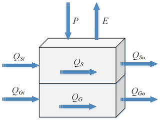
The exchange of water between non-channel grid cells is illustrated in Fig. 8, where P and E are the rainfall and the evaporation in the grid cell, Q_Si and Q_Gi are the surface runoff inflow and the underground runoff inflow from the upstream grid cell, Q_S and Q_G are the surface runoff and the groundwater runoff, and Q_So and Q_Go are the surface and the groundwater runoff outflow to the downstream grid cell.

Figure 8 The water exchange processes in a non-channel grid cell.

As mentioned, when the rainfall intensity in the grid cell is greater than the infiltration capacity, the surface runoff Q_S occurs in this cell. If the upstream cell also generates the surface runoff Q_Si, the surface runoff outflow Q_So can be calculated as

$$\begin{array}{}\text{(7)}& Q_{\mathrm{So}}=Q_{\mathrm{Si}}+Q_{\mathrm{S}}.\end{array}$$

As part of the groundwater runoff from the upstream grid cell supplements the soil water storage, the ratio of which is set as “sc”; the groundwater runoff outflow Q_Go is calculated as

$$\begin{array}{}\text{(8)}& Q_{\mathrm{Go}}=Q_{\mathrm{Gi}}\times (\mathrm{1}-\mathrm{sc})+Q_{\mathrm{G}}.\end{array}$$

The soil water storage of the grid cell $P_{{\mathrm{a}}_t}$ at the end of the period t is

$$\begin{array}{}\text{(9)}& P_{{\mathrm{a}}_t}=P_{{\mathrm{a}}_{t-\mathrm{1}}}+Q_{\mathrm{Gi}}\times \mathrm{sc}.\end{array}$$

If the soil water storage $P_{{\mathrm{a}}_t}$ is greater than the storage capacity of the grid cell, then let $P_{{\mathrm{a}}_t}$ equal to the soil moisture capacity.

(2) Exchange of water in a channel grid cell

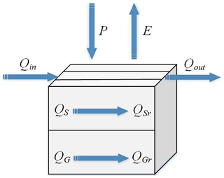
For the exchange of water in a channel grid cell, the generated surface and groundwater runoff is no longer supplied directly to the downstream cell, but imported to the river channel and passes through the channel routing to the next cell. The processes are as illustrated in Fig. 9; the symbols of which have the same meanings as Fig. 8.

Figure 9 The water exchange processes in a channel grid cell.

With the rainfall P and the evaporation E, the surface runoff Q_S and the groundwater runoff Q_G are generated. Based on the flow routing, the surface and the groundwater inflow to the river channel Q_Sr and Q_Gr can be obtained. The generated total inflow Q_c of the channel grid is then calculated as

$$\begin{array}{}\text{(10)}& Q_{\mathrm{c}}=\left(Q_{\mathrm{Sr}}+Q_{\mathrm{Gr}}\right)\times \mathit{\epsilon },\end{array}$$

where ε is the proportional coefficient of the surface and the groundwater runoff into the river channel. By adding Q_in and Q_c, the outflow of the channel grid cell Q_out to the downstream cell can be obtained as

$$\begin{array}{}\text{(11)}& Q_{\mathrm{out}}=Q_{\mathrm{in}}+Q_{\mathrm{c}}.\end{array}$$

3.2.3 Confluence calculation and channel seepage

The storage–discharge relation of grid cell can be simplified to a single-line form. The storage–discharge equation can be obtained as

$$\begin{array}{}\text{(12)}& S={\displaystyle \frac{A}{\mathrm{1}-\mathit{\omega }}}{Q}^{\mathrm{1}-\mathit{\omega }},\end{array}$$

where S is water storage (m³), Q is the outflow rate (m³ s⁻¹), A is the confluence parameter, and ω is the shape parameter. According to the water balance equation

$$\begin{array}{}\text{(13)}& {\displaystyle \frac{\mathrm{d}S}{\mathrm{d}t}}=I-Q,\end{array}$$

the outflow rate of the grid cell Q_t at the end of the period t (Goutal and Sainte-Marie, 2011) is

$$\begin{array}{}\text{(14)}& \begin{array}{rl}& Q_t=\\ & \left\{\begin{array}{ll}{Q}_{t-\mathrm{1}}{\left(\mathrm{1}+\frac{\mathit{\omega }}{A}{Q}_{t-\mathrm{1}}^{\mathit{\omega }}\right)}^{-\frac{\mathrm{1}}{\mathit{\omega }}}& I_{t-\mathit{\tau }}=\mathrm{0}\\ {\left[\mathrm{0.5}{\left(\mathrm{16}{A}^{\mathrm{2}}+\mathrm{8}{I}_{t-\mathit{\tau }}+\mathrm{16}A{Q}_{t-\mathrm{1}}^{\mathrm{0.5}}-\mathrm{4}{Q}_{t-\mathrm{1}}\right)}^{\mathrm{0.5}}-\mathrm{2}A\right]}^{\mathrm{2}}& \mathit{\omega }=\mathrm{0.5}\\ e^{\left(\frac{I_{t-\mathit{\tau }}-\mathrm{0.5}{Q}_{t-\mathrm{1}}+S_{t-\mathrm{1}}+A\ln Q_{t-\mathrm{1}}-\mathrm{0.5}{Q}_t}{A}\right)}& \mathit{\omega }=\mathrm{1}\\ \left[\frac{I_{t-\mathit{\tau }}-\mathrm{0.5}{Q}_{t-\mathrm{1}}+D{Q}_{t-\mathrm{1}}^{\mathrm{1}-\mathit{\omega }}-\mathrm{0.5}{Q}_t}{D}\right]& \mathit{\omega }\ne \mathrm{1},\end{array}\right.\end{array}\end{array}$$

where I is the inflow rate (m³ s⁻¹), I_t−τ is the inflow rate (m³ s⁻¹) at time t−τ (τ is the travel time of flood wave), and D can be expressed as

$$\begin{array}{}\text{(15)}& D={\displaystyle \frac{A}{(\mathrm{1}-\mathit{\omega })\mathrm{\Delta }t}},\end{array}$$

where Δt is the calculation time interval (s).

Due to the perennial water shortage and extensive channel seepage in study site, Horton infiltration model is applied to obtain the infiltration volume. When the calculation interval is 1 h, the infiltration volume can be calculated by the following equation (Horton, 1933):

$$\begin{array}{}\text{(16)}& f=\left(f_{\mathrm{0}}-f_{\mathrm{c}}\right)\cdot e^{-kt}+f_{\mathrm{c}},\end{array}$$

where f₀ is the initial infiltration rate (mm h⁻¹), and k is a parameter about soil. The channel seepage should be deducted before channel confluence is calculated with Eq. (14).

3.2.4 Discretization method for the soil moisture storage capacity and the infiltration capacity

In a grid-type hydrological model, it is necessary to determine the soil moisture storage capacity and infiltration capacity in the grid cells in order to calculate the runoff generated within the grid and to simulate the generation and convergence of runoff in the river basin. Therefore, the determination of soil moisture storage capacity and infiltration capacity are key to model construction. Beven and Kirky (1979) proposed a topography-based semi-distributary hydrological model (TOPMODEL) that fully considered the effects of topography on the formation and change of runoff areas, using the spatial distribution of the terrain index ln (α∕tan β) to reflect the spatial distribution of saturated and deficit water volumes in the river basin. Based on this theory, it can be assumed that areas with similar topographic indices have the same hydrological response.

According to a statistical analysis of topographic indices for the 1 km×1 km, 3 km×3 km, and 9 km×9 km grids in the Fuping and Zijingguan basins, the cumulative distribution curves of the different grids' topographic indices in the same area have the same shape (parabolic). However, the cumulative distribution curve of topographic indices between different areas is also very similar. Experimentation showed that the soil moisture storage capacity and infiltration capacity of different grids can be obtained and dispersed using the topographic indices as follows:

$$\begin{array}{}\text{(17)}& {\displaystyle \frac{W_i}{\mathrm{WMM}}}=\exp \left\{-{\left[{\displaystyle \frac{\ln \left({\mathrm{TI}}_{\mathrm{i}}-{\mathrm{TI}}_{\min }+\mathrm{1}\right)}{\mathit{\alpha }}}\right]}^{\mathit{\beta }}\right\},\end{array}$$

where W_i is the moisture storage capacity of a certain grid cell (mm), WMM is the maximal moisture storage capacity of a certain grid cell, TI_i is the topographic index of the grid, TI_min is the topographic index of the minimum point in the basin, α is the scale parameter of the grid, and β is the shape parameter of the grid.

$$\begin{array}{}\text{(18)}& {\displaystyle \frac{f_{\mathrm{i}}}{f_{\mathrm{m}}}}={\left\{\mathrm{1}-{\left[\mathrm{1}-\exp [-{\displaystyle \frac{\mathrm{1}}{\mathit{\alpha }}}{\left[\ln \left(T_{\mathrm{i}}-{\mathrm{TI}}_{\min }+\mathrm{1}\right)\right]}^{\mathit{\beta }}\right]}^b\right\}}^{\mathrm{1}/n},\end{array}$$

where f_i is the infiltration capacity of a certain grid cell in the river basin, and f_m is the infiltration capacity of the maximum point in the basin.

3.3 Establishment of coupled atmospheric–hydrologic systems

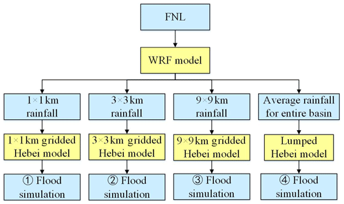
Either one-way or two-way coupling can be achieved. For the latter, it is necessary to establish a communication mechanism between the atmospheric and hydrologic models to allow both to respond and combine dynamically. However, this process requires more complicated mechanisms and a higher amount of supportive data, making this approach difficult to use widely in actual forecasting, so this study focuses on one-way coupling. In order to research coupling scales, it is necessary to establish a gridded atmospheric–hydrologic coupled system. The WRF model is used to generate gridded rainfall data, and the gridded Hebei model is used as the land surface hydrologic model. The latter is set up with different grid divisions to allow the retrieval of rainfall data with a corresponding precision from the output data of the WRF model. Differences in the output processes of the hydrological models at different scales are then analyzed, and the relationships between the differences and rainfall patterns are considered. The lumped Hebei model is also used to establish the lumped atmospheric–hydrologic coupled system. The gridded rainfall data from the WRF model are averaged over each sub-watershed, which is regarded as the input of the lumped Hebei model. The coupled atmospheric–hydrologic system is illustrated in Fig. 10.

Figure 10 The coupled atmospheric–hydrologic system.

The gridded Hebei model is divided into the three different grid sizes noted above. The coordinates of the grid cell centers could be used to retrieve the corresponding output data from the WRF model for driving the hydrologic model. The SCE-UA (shuffled complex evolution) method (Duan et al., 1994) is used to calibrate the parameters, and the calibrated values are shown in Table 6. Due to the limited observational data, seven storm events in Fuping and six storm events in Zijingguan are selected and used to calibrate the Hebei model, and another two from each sub-watersheds are used for model validation. In order to guarantee reasonable values for the initial model conditions, the storm events are not independently used but rather with an antecedent period of data with the length of 15 days before the start of the event. The validation results show an average Nash–Sutcliffe efficiency coefficient (NSE) value of up to 0.686, indicating the calibrated models are reliable for further applications. It should be noted that the four storm events in Sect. 2.2 are different from those used for calibration and validation.

3.4 Evaluation statistics

The flood simulation results are evaluated using three statistics: the relative flood peak error (R_f), the relative flood volume error (R_l), and the Nash–Sutcliffe efficiency coefficient (NSE).

$$\begin{array}{}\text{(19)}& {\displaystyle }& {\displaystyle }{R}_{\mathrm{f}}=\left(Q_{\mathrm{f}}^{\prime }-Q_{\mathrm{f}}\right)/Q_{\mathrm{f}}\text{(20)}& {\displaystyle }& {\displaystyle }{R}_{\mathrm{l}}=\left(Q_{\mathrm{l}}^{\prime }-Q_{\mathrm{l}}\right)/Q_{\mathrm{l}}\text{(21)}& {\displaystyle }& {\displaystyle }\mathrm{NSE}=\mathrm{1}-{\displaystyle \frac{\sum _{i=\mathrm{1}}^N{\left(Q_i^{\prime }-Q_i\right)}^{\mathrm{2}}}{\sum _{i=\mathrm{1}}^N{\left(Q_i-\stackrel{\mathrm{‾}}{Q}\right)}^{\mathrm{2}}}},\end{array}$$

where $Q_{\mathrm{f}}^{\prime }$ and Q_f are the simulated and observed flood peak flow, $Q_{\mathrm{l}}^{\prime }$ and Q_l are the simulated and the observed flood volume, $Q_i^{\prime }$ and Q_i are the simulated and observed flow discharge at the ith time step, N is the total time steps of the flood event, and $\stackrel{\mathrm{‾}}{Q}$ is the average value of Q_i at each time step.

4 Results

4.1 Simulation results of the coupled atmospheric–hydrologic systems

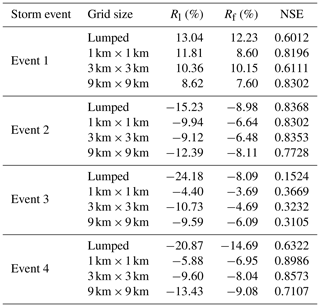
The coupled atmospheric–hydrologic systems mentioned in Sect. 3.3 are used to simulate the four storm events. The flood processes at different grid divisions are retrieved by the gridded atmospheric–hydrologic coupled system, and the comparison is also made with the results from the lumped atmospheric–hydrologic coupled system. As shown in Fig. 11 and Table 7, the lumped system performs worse than the gridded system in most cases. The simulation results of the lumped system are close to the gridded system with different grid divisions for storm events 1 and 2, while the simulation results have a significant difference between lumped system and grid system for storm events 3 and 4. The gridded system, especially with the 1 km×1 km and 3 km×3 km grid, can improve accuracy and reduce error in the flood simulation for event 4.

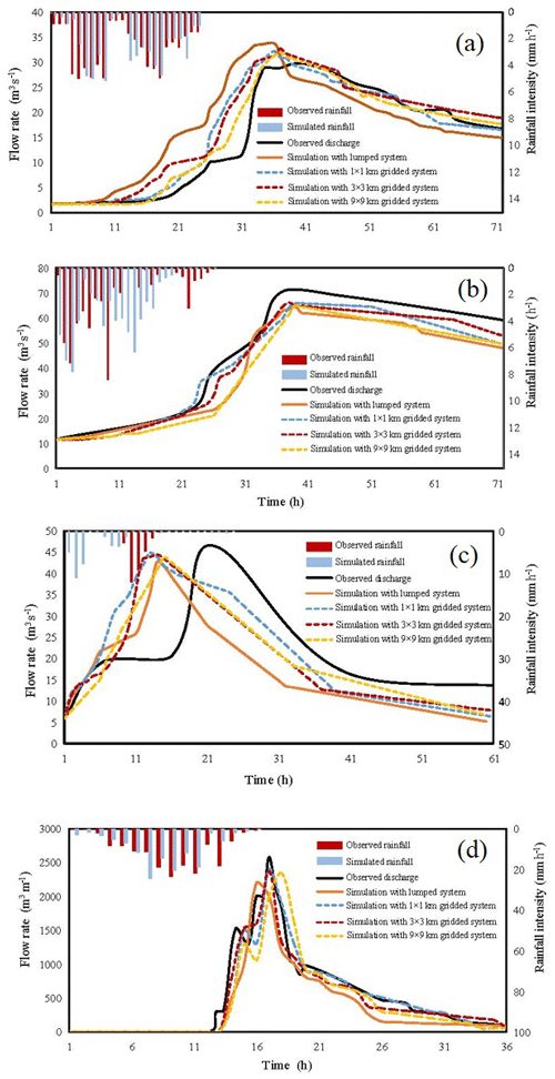
Figure 11 Flood process simulations of the coupled atmospheric–hydrologic systems for the four storm events: (a) event 1 in Fuping, (b) event 2 in Fuping, (c) event 3 in Fuping, and (d) event 4 in Zijingguan.

Table 7 Simulation results of the coupled atmospheric–hydrologic systems for four storm events.

The simulated results based on different grid sizes are similar for storm event 1, though the 9 km×9 km grid has the optimal simulation performance. All the coupled atmospheric–hydrologic systems at different grid divisions perform well for storm event 2, and the 3 km×3 km grid produces the optimal simulation result. For storm event 3 (a short-duration heavy rainfall), although the peak flow error and flood volume error are not significant, the simulation results fail to truly reflect the runoff process. The 1 km×1 km grid generates the optimal simulation result for storm event 4.

It can be easily found that different rainfall events have different simulation results with the three grid sizes. The absolute value of R_f is within 3.69 %–8.60 % for the system with 1 km resolution, 4.69 %–10.15 % for the system with 3 km resolution, and 6.09 %–9.08 % for the system with 9 km resolution. The absolute value of R_l ranges from 4.40 % to 11.81 % for the system with 1 km resolution, ranges from 9.12 % to 10.36 % for the system with 3 km resolution, and ranges from 8.62 % to 13.43 % for the system with 9 km resolution. The NSE is from 0.3669 to 0.8986 for a 1 km×1 km grid, from 0.3232 to 0.8573 for a 3 km×3 km grid, and from 0.3105 to 0.8302 for a 9 km×9 km grid. Considering the rainfall simulation errors from the WRF model for storm event 3, the 1 km×1 km and 3 km×3 km grids provide better simulation results overall, while the 9 km×9 km grid leads to unstable variations over a wide area. However, for a specific storm event, higher resolution may not lead to better flood process simulation. For example, the 9 km×9 km grid provides the optimal simulation results for storm event 1, while the best grid size is 3 km×3 km for rainfall event 2.

4.2 Relationship between the rainfall evenness and the performance of the gridded model with different grid size

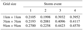
Considering the characteristics of the spatial rainfall distributions, the gridded rainfall simulation results from the WRF model are more suitable for the application of the gridded Hebei model than lumped Hebei model. In order to analyze the relationship between the rainfall evenness and the performance of the gridded model with different grid size, the C_v values are calculated for the rainfall simulations from the WRF model. Table 8 shows that there is not much difference among the C_v values with different grid size for the same storm event, while the difference is obvious for different storm events. The ranking of the spatial evenness of the rainfall simulations is event 1 > event 2 > event 3 > event 4.

Table 8 C_v values of simulated rainfall spatial distribution for the four storm events.

Table 9 Comparison between gridded system and lumped system for flood simulation results.

The average flood simulation results (${\stackrel{\mathrm{‾}}{R}}_{\mathrm{l}}$, ${\stackrel{\mathrm{‾}}{R}}_{\mathrm{f}}$, and $\stackrel{\mathrm{‾}}{\mathrm{NSE}}$) for different grid size are calculated and used to compare with the flood simulation results (R_l-lumped, R_f-lumped, and NSE_-lumped) of the lumped system (shown in Table 9). Due to the large error in the rainfall simulation, storm event 3 is used as a reference event for further comparisons in this study. For the other three storm events, the difference between the gridded system and lumped system becomes more significant as the heterogeneity of the rainfall spatial distribution increases. In other words, when the spatial distribution of the rainfall is uniform, as events 1 and 2, both the lumped and gridded systems achieve good simulation results. The simulation results of the former are even superior to those of the latter in some cases, such as the NSE for event 2. However, when the spatial distribution of the rainfall is uneven, the lumped system in most cases could only simulate the overall runoff situation but fails to fully describe the runoff process, while the gridded system could obtain a better simulation, such as for event 4. Furthermore, the 3 km×3 km grid produces the most stable simulation results for events 1 and 2, which have the evenly distributed rainfall in space. It means that the simulation results may not always be improved with higher-dimension precision and a more complicated system. As the spatial distribution of rainfall becomes uneven, the simulated effect with 9 km×9 km grid declines quickly, and other grid sizes lead to better flood process simulation. The simulation results tend to improve with higher-dimension precision.

Table 10 Simulation results of the coupled atmospheric–hydrologic systems based on the corrected gridded rainfall for four storm events.

5 Discussion

The errors in the rainfall simulation from the WRF model have a significant influence on the coupled atmospheric–hydrologic modeling system. Do the above conclusions change if the rainfall errors were eliminated? It is necessary to analyze the flood simulation results driven by the simulated rainfall, which is corrected by the measured values from the rain gauges. We assume that the WRF model is able to capture the spatial patterns of the simulated rainfall. The Thiessen polygon method is used to divide the control region of each rain gauge. The areal rainfall of the control region based on the rain gauge is regarded as the true rainfall value, which is allocated by the spatial distribution ratio from the simulated rainfall. The average value of the corrected gridded rainfall should be equal to the measured value of the rain gauge in a specific control region.

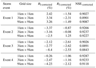
The corrected gridded rainfall is used to drive the coupled atmospheric–hydrologic modeling system, and the simulation results are shown in Table 10. The system obtains similar simulation results of the three different grid sizes for events 1 and 2. It is hard to say which grid division is the most outstanding, and higher resolution may not lead to better flood process simulation. The corrected rainfall leads to much better flood process simulations than the uncorrected rainfall from the WRF model. The simulations have significant improvement by using the corrected rainfall for event 3, and the system can reproduce the flood process. The NSE_-corrected values are all above 0.88, and the R_f-correctedvalues are all lower than 3 % at different grid sizes. The system with low R_f-corrected and R_l-corrected and high NSE_-corrected also performs well with different grid divisions for event 4. Higher resolution can lead to better flood process simulation for events 3 and 4. The system with 1 km×1 km grid size has the best simulation result. The conclusions are similar for both the corrected rainfall and the uncorrected rainfall. It is not always better for higher resolution, and the grid size selection has a strong relationship with the rainfall evenness. Considering the study only focusing on two semi-humid and semi-dry watersheds with limited storm events involved, the results in this study should be verified by more case studies before more general conclusions can be achieved.

Table 11 The system errors from the rainfall simulations for four storm events.

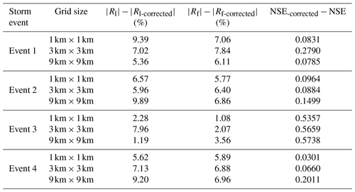
Comparing the results from Tables 7 and 10, the system errors from the rainfall simulations (as shown in Table 11) can be easily obtained by the subtraction of the corresponding values in Tables 7 and 10. For event 1, the average $\left|R_{\mathrm{l}}\right|-\left|R_{\mathrm{l}\text{-}\mathrm{corrected}}\right|$, $\left|R_{\mathrm{f}}\right|-\left|R_{\mathrm{f}\text{-}\mathrm{corrected}}\right|$, and NSE_-corrected−NSE of the three different grid sizes caused by the rainfall simulations are 7.26 %, 7.00 %, and 0.1469. In the same way, the average $\left|R_{\mathrm{l}}\right|-\left|R_{\mathrm{l}\text{-}\mathrm{corrected}}\right|$, $|R_{\mathrm{f}}-|R_{\mathrm{f}\text{-}\mathrm{corrected}}|$, and NSE_-corrected−NSE of the three grid sizes are 7.47 %, 6.34 %, and 0.1116 for event 2. A notable case is event 3. $\left|R_{\mathrm{l}}\right|-\left|R_{\mathrm{l}\text{-}\mathrm{corrected}}\right|$ of event 3 with the grid size 3 km×3 km (7.96 %) is the highest among the three grid sizes, and the highest $\left|R_{\mathrm{f}}\right|-\left|R_{\mathrm{f}\text{-}\mathrm{corrected}}\right|$ (3.56 %) comes from the grid size 9 km×9 km. Due to the errors in the rainfall simulations, all the NSEs decline by more than 0.5 for the three grid sizes. For event 4, the average $\left|R_{\mathrm{l}}\right|-\left|R_{\mathrm{l}\text{-}\mathrm{corrected}}\right|$, $\left|R_{\mathrm{f}}\right|-\left|R_{\mathrm{f}\text{-}\mathrm{corrected}}\right|$, and NSE_-corrected−NSE of the three grid sizes caused by the rainfall simulations are 7.32 %, 6.58 %, and 0.0991. It can easily be found that the magnitudes of most errors in Table 11 are higher than those of Table 10, which indicates that the accuracy of the simulated rainfall is the main factor affecting the performance of the coupled system. In order to improve the rainfall simulation in small- and medium-scale catchments, radar data with high spatiotemporal resolution should be a good choice, such as radar quantitative precipitation estimates (QPE) or quantitative precipitation forecasts (QPF) and radar data assimilation for the NWP model (Xiao and Sun, 2007; Harader et al., 2012; Dai et al., 2019).

It should be mentioned that there is a necessity to incorporate parameter uncertainty analysis in this study. However, this will need a considerable set of the observational data (Hughes et al., 2010). Due to the lack of sufficient historical storm–flood processes, it is impossible to carry out such analyses. Nevertheless, parameter uncertainty estimations and ensemble simulations with perturbed parameters are suggested for future study when sufficient observational data are available.

6 Conclusion

This study establishes a coupled atmospheric–hydrologic modeling system with variable grid sizes in sub-humid and sub-arid area in northern China. The choice of coupling scales (1 km×1 km, 3 km×3 km, 9 km×9 km) is discussed in depth. The WRF model and the gridded Hebei model are used to establish the gridded atmospheric–hydrologic coupled system. The lumped Hebei model is also used to establish the lumped atmospheric–hydrologic coupled system, and the simulation result serves as a reference.

Contrastive analyses of the flood process simulations from the gridded atmospheric–hydrologic coupled system and the lumped atmospheric–hydrologic coupled system are carried out. Four main conclusions can be drawn: (1) the lumped system performs worse than the gridded system in most cases, while the simulation results are close to the gridded system for the storm events with uniform spatial distribution; (2) the coupled atmospheric–hydrologic systems at different grid divisions obtain similar simulation results and perform well for the storm events with uniform spatial distribution; (3) the simulation results may not always be improved with higher-dimension precision, and the grid size selection should considering the rainfall evenness; and (4) for the storm events with uneven spatiotemporal distribution, the corrected rainfall can improve the simulation results significantly, and higher resolution can lead to better flood process simulation. Flood forecasting is a stress and difficulty in the sub-humid and sub-arid area in northern China. The coupled atmospheric–hydrologic modeling system is influenced by the rainfall forecast accuracy and physics mechanisms of a hydrologic model. Further research considering the improvement of rainfall forecast and hydrologic models should be carried out to further verify the conclusions of this study.