Neighbourhood and stand structure affect stemflow generation in a heterogeneous deciduous temperate forest

Although stemflow oftentimes only represents a small portion of net precipitation in forests, it creates hot spots of water input that can affect subsurface storm-flow dynamics. The distribution of stemflow over different trees is assumed to be temporally stable, yet often unknown. Therefore, it is essential to know the systematic factors driving stemflow patterns. Several drivers have been identified in the past, mainly related to tree traits. However, less attention has been paid to tree neighbourhood interactions impacting stemflow generation and creating stand patches with enhanced or reduced stemflow.

We recorded stemflow during 26 precipitation events on 65 trees, growing in 11 subplots (100 m² each), in a temperate mixed beech forest in the Hainich National Park, Germany. We used linear mixed effects models to investigate how traits of individual trees (tree size, tree species, number of neighbouring trees, their basal area and their relative height) affect stemflow and how stemflow is affected by stand properties (stand, biomass and diversity metrics).

As expected, stemflow increased with event and tree size. Stemflow was highly variable at both the tree and subplot scale. Especially in large rainfall events (>10 mm), the tree/subplot ranking was almost identical between events, probably due to fully developed flow paths bringing out the full stemflow potential of each tree. Neighbourhood and stand structure were increasingly important with event size (15 % of fixed effects on the tree scale and ca. 65 % on the subplot scale for large events). Subplot-scale stemflow was especially enhanced by a higher proportion of woody surface, expressed by a high number of trees, low leaf area and a large maximum tree size. The Simpson diversity index contributed positively to stemflow yield for large events, probably by allowing more efficient space occupation. Furthermore, our models suggest that the neighbourhood impacts individual tree morphology, which may additionally increase stemflow in dense, species diverse neighbourhoods. Unexpectedly, rain shading within the canopy had little impact on the stemflow spatial variation.

Overall, we find a strong cross-scale temporal stability. Tree size and tree density were the main drivers, independently increasing stemflow, creating forest patches with strongly enhanced or reduced stemflow. Our results show that, besides tree metrics, forest structure and tree diversity also affect stemflow patterns and the potentially associated biogeochemical hot spots.

1 Introduction

In forests, precipitation is intercepted by the canopy and reaches the soil partitioned into throughfall and stemflow. The different pathways of precipitation through the forest canopy create a strongly heterogeneous pattern of water input to the soil, with consequences for soil hydrobiochemistry (Levia and Frost, 2003; Zimmermann et al., 2007). These pathways compartmentalize the forest floor into cold and hot spots of infiltration, with a strong subsequent impact on subsurface flow and biogeochemical processes (Liang et al., 2007; Guswa and Spence, 2012; Coenders-Gerrits et al., 2013). Thus, an understanding of forest canopy precipitation partitioning processes is highly important for our conceptual understanding of forest ecohydrology systems.

Although stemflow constitutes a minor fraction of net precipitation, research shows that stemflow is important for a site's hydrological functioning (Pressland, 1976; Durocher, 1990; Levia and Frost, 2003; Hildebrandt et al., 2007; Staelens et al., 2008; Levia and Germer, 2015; Carlyle-Moses et al., 2018). Stemflow introduces a strong additional heterogeneity to subcanopy precipitation. Stems potentially act as funnels and can make trees prominent hot spots of canopy drainage. Concentrated water inputs to the soil can trigger macropore flow (Flühler and Roth, 2004), bypassing the soil and thresholding subsurface storm-flow processes that contribute to deep percolation (Taniguchi et al., 1996; Liang et al., 2007). This effect has been called double-funnelling of trees (Martinez-Meza and Whitford, 1996; Johnson and Lehmann, 2006; Li et al., 2009; Liang et al., 2011; Schwärzel et al., 2012) and renders trees important players in the hydrological functioning of forests, on top of their role with respect to soil water depletion.

Correctly depicting variance of stemflow and understanding its mechanisms can be of utter importance, because according to the hot spots and hot moments hypotheses (McClain et al., 2003), maximum fluxes have the strongest impact on the system (rather than site averages). However, few studies have provided measures of stemflow spatial (i.e. tree-to-tree) variation (Hanchi and Rapp, 1997; Zimmermann et al., 2015). Most stemflow studies focus on a few trees to exemplify a site's possible stemflow processes. This is probably because elaborate sampling is required to capture stemflow variance: a random and representative sample is needed, encompassing a high coverage and extent within the study stand. The limited data that are available show that stemflow variation is substantial, and higher for stemflow than for throughfall (Metzger et al., 2017; van Stan et al., 2019). Thus, stemflow contributes importantly and even primarily to net precipitation heterogeneity and flux hot and cold spots and moments. At the same time, some research suggests that tree-to-tree stemflow variation is stable in time (Metzger et al., 2017), meaning that during different precipitation events, the same trees produce relatively high or relatively low stemflow. Although few studies have explicitly investigated this temporal stability in stemflow, a great deal of research has been conducted to link tree traits to stemflow yield to understand spatial (i.e. tree-to-tree) variability, and thus inherently implied temporally stabile drivers. Most prominently, tree diameter (or circumference, basal area, crown projection area) has been identified as a factor shaping tree-specific stemflow within an event (Reynolds and Henderson, 1967; Aboal et al., 1999; André et al., 2008; Krämer and Hölscher, 2009; Takahashi et al., 2011). However, stemflow yield still shows a great deal of between-tree variation after accounting for tree size (Reynolds and Henderson, 1967; Takahashi et al., 2011; McKee and Carlyle-Moses, 2017), as trees' traits related to morphology and crown architecture additionally affect individual tree stemflow. For example, factors such as many and steeply inclined branches (Herwitz, 1987; Návar, 1993; Iida et al., 2005; Levia et al., 2015; Martinez-Meza and Whitford, 1996), smoother bark (Aboal et al., 1999; Iida et al., 2005; van Stan and Levia, 2010; van Stan et al., 2016), leaf hydrophobicity (Iida et al., 2005), low LAI/few leaves (Takahashi et al., 2011; Molina and del Campo, 2012; Levia et al., 2015) and more woody surface (Levia and Germer, 2015; Levia et al., 2015) have been found to enhance stemflow production.

So far, most of the investigations have targeted species-specific variables. However, some canopy traits are also affected by stand structure: trees have been shown to strongly adapt their growth to the space occupation of neighbouring trees (Schröter et al., 2012; Juchheim et al., 2017). Different competition strategies and typical phenotypes of different species complement each other in mixed forest, allowing for more efficient niche and space occupation (Frech et al., 2003; Juchheim et al., 2017). Thus, neighbourhood characteristics such as species composition, diversity or size heterogeneity could also impact tree traits related to stemflow. Stand and neighbourhood properties might directly and indirectly influence stemflow formation of the individual tree. This pattern could also persist on a larger scale, forming forest patches of structure-induced enhanced and reduced stemflow.

Nevertheless, neighbourhood effects have hardly been considered for stemflow analyses. Some studies have included canopy position, (Reynolds and Henderson, 1967; Aboal et al., 1999; Terra et al., 2018) or neighbouring tree proximity (McKee and Carlyle-Moses, 2017) in tree stemflow models, whereas Krämer and Hölscher (2009) tested species composition effects on area average stemflow. Other studies have discussed a shading effect in the lower canopy (André et al., 2008; Takahashi et al., 2011) as a possible explanation for their stemflow results. However, a systematic study explicitly focusing on neighbourhood effects on stemflow in a quantitative approach is currently missing.

In this contribution, we tackle spatio-temporal patterns of stemflow in conjunction with spatially distributed tree and neighbourhood variables using a spatially stratified design. Additionally, by assessing stemflow area based on 11 small (100 m²) subplots, we obtain a first assessment of effects impacting areal integrated stemflow patterns at the subplot scale.

Based on the above design, we assess the temporal stability of spatial stemflow patterns and test the impacts of stand structure and neighbourhood parameters (additional to tree size) on individual stemflow yield as well as whether these factors even out for stemflow variation at a larger scale.

2 Methods

2.1 Site description and sampling design

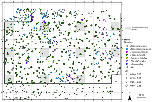
The measurement site is situated in a gently sloping forested area in the Hainich low mountain range in central Germany. It is a site of the Hainich Critical Zone Exploratory within the Collaborative Research Center AquaDiva (Küsel et al., 2016). Annual rainfall ranges between 600 and 900 mm. The mixed beech forest is part of a national park and is unmanaged, with a high age and species heterogeneity. Within a 1 ha sampling plot, 11 respective subplots of 10 m × 10 m were chosen in a regular pattern and stemflow was measured on all trees within the subplots (Fig. 1). A total of 65 trees were such selected with the following species composition: 80 % were beech trees (Fagus sylvatica), 12 % were sycamore maple (Acer pseudoplatanus), and Acer platanoides, Fraxinus excelsior, Carpinus betulus and Ulmus glabra also occurred. The diameter at breast height (DBH) showed a negative exponential distribution, with 54 % of the trees having a DBH that was less than 0.1 m and a maximum DBH of 0.81 m. Tree metrics within the subplots were representative of the larger-scale stand (see Appendix).

Figure 1 Position of the 11 subplots (grey shaded areas, 10 m × 10 m) in which stemflow was sampled within the forest plot.

2.2 Field sampling

2.2.1 Measurement of stand properties

Trees within the plot and a 10 m buffer zone around the plot were surveyed and given and identification number (ID). The position of each tree was determined using a total station (Topcon, Tokyo, Japan) combined with a differential GPS (Topcon, Tokyo, Japan). Tree height was measured using an ultrasonic sensor (Haglöf Vertex, Haglöf, Järfälla, Sweden), and tree circumference at breast height was measured with a measuring tape in 2014. The trees' DBH and basal area values were calculated from their circumference at breast height, assuming a circular tree trunk. The leaf area index was measured in summer 2015 using an LAI-2000 (LI-COR, Lincoln, Nebraska USA).

2.2.2 Neighbourhood of individual trees

From the stand properties we derived metrics describing the neighbourhood of the 65 individual trees. “Neighbourhood” was defined as the area around the tree with a radius of the mean tree distance on the plot:

$$\begin{array}{}\text{(1)}& r=\mathrm{2}\sqrt{{\displaystyle \frac{\frac{A_{\mathrm{plot}}}{n_{\mathrm{trees},\mathrm{plot}}}}{\mathit{\pi }}}},\end{array}$$

where r is the mean tree distance (which equals 4.7 m on our plot), A_plot is the plot area and n_trees,plot is the total number of trees on the plot. Within this radius, we counted the number of trees in the neighbourhood, their cumulative basal area, and the neighbourhood's relative height (h_n,rel), as follows:

$$\begin{array}{}\text{(2)}& h_{\mathrm{n},\mathrm{rel}}={\displaystyle \frac{h_{\mathrm{tree},\max }}{h_{\mathrm{tree},j}}},\end{array}$$

where h_tree,max is the height of the highest tree in the neighbourhood, and h_tree,j is the height of reference tree j. Note that relative height, as a neighbourhood property, increases for taller neighbourhoods.

2.2.3 Subplot characteristics

We calculated heterogeneity measures for each stemflow subplot. We used the Simpson index of biodiversity D (Simpson, 1949), as it is suitable for small sample sizes, −log _eD transformed, as recommended by Buckland et al. (2005):

$$\begin{array}{}\text{(3)}& D={\sum }_i{\left({\displaystyle \frac{n_i}{{\sum }_i{n}_i}}\right)}^{\mathrm{2}},\end{array}$$

where n_i is the number of individuals of species i per unit area.

Additionally, we derived a size heterogeneity index H, which was calculated according to Krämer and Hölscher (2009) as

$$\begin{array}{}\text{(4)}& H={\displaystyle \frac{\frac{q_{\mathrm{0.75},s}-q_{\mathrm{0.25},s}}{q_{\mathrm{0.5},s}}}{\stackrel{\mathrm{̃}}{s}}},\end{array}$$

with

$$\begin{array}{}\text{(5)}& s=h_{\mathrm{tree}}{d}_{\mathrm{tree}},\end{array}$$

Here q_x,s is the xth quantile of s, and h_tree and d_tree are the height and DBH of a tree respectively.

2.2.4 Gross precipitation and stemflow measurement

Gross precipitation and stemflow were measured as described in Metzger et al. (2017). For gross precipitation, five funnel-type collectors were used, which were placed ca. 250 m from the forest plot on an adjacent grassland, ca. 50 m from the forest edge. Precipitation (in mm) was derived by referring the precipitation volume in the collectors to the area covered by the funnel and taking the median of the five parallel measurements.

Stemflow was collected on all trees within the 11 designated subplots (see above) into containers by way of collars made from lay-flat hose wrapped around the trees and sealed with silicone. Precipitation was sampled on an event basis from May to August in the years 2014, 2015 and 2016, recording all occurring events. Sampling started ca. 2 h after the event ended. Measurements lasted several hours. If measurements were interrupted by new rainfall, events were treated cumulatively. Over the entire period a total 39 events were recorded. Events during which overflow of containers could have occurred for at least one stemflow measurement were excluded from the data analysis. For the statistical model analysis (see below), we also excluded very small events (<0.5 L median stemflow per tree), leaving 26 of the 39 sampled precipitation events. Subplot stemflow was calculated as the sum of stemflow collected from all trees on that subplot.

The stemflow funnelling ratios were calculated from the individual stemflow volumes as follows (Herwitz, 1987):

$$\begin{array}{}\text{(6)}& R_{\mathrm{F}}=\left({\displaystyle \frac{V_{\mathrm{SF}}}{P_{\mathrm{g}}\cdot A_{\mathrm{tree}}}}\right),\end{array}$$

where R_F is the funnelling ratio, V_SF is the stemflow volume, P_g is the gross precipitation and A_tree is a tree's basal area. It shows, the degree to which a tree concentrates the rainfall to a point water input to the soil.

Normalized tree/subplot stemflow V_SFn was calculated from the individual tree stemflow volume ($V_{\mathrm{SF},j,e}$) for event e, and the event's median stemflow volume ($\stackrel{\mathrm{̃}}{V_{\mathrm{SF},e}}$), according to Vachaud et al. (1985):

$$\begin{array}{}\text{(7)}& V_{\mathrm{SFn}}=\left({\displaystyle \frac{V_{\mathrm{SF},j,e}-\stackrel{\mathrm{̃}}{V_{\mathrm{SF},e}}}{\stackrel{\mathrm{̃}}{V_{\mathrm{SF},e}}}}\right).\end{array}$$

2.3 Statistical analysis

2.3.1 Descriptive statistics of stemflow patterns

To examine temporal stability of stemflow patterns, we correlated individual/subplot stemflow yields pairwise for all events falling into an event size class, thereby obtaining a set of correlation coefficients for each event size class. In order to account for non-normal distribution of stemflow, we used Spearman rank correlations. Thus, sets of high (or low) correlation coefficients signify that the same (or different) trees/subplots produce above and below average stemflow yields during each event, demonstrating high (or low) temporal stability.

2.3.2 Linear mixed effects models

In order to determine the effect of potential driving factors for stemflow yield, linear mixed effects models (LMMs) were used. LMMs are multivariate linear regression models that allow the user to control for repeated sampling. Quantified factors, the impact of which is to be tested in the model, are called fixed effects. Qualitative information of repeated sampling, referring to individuals, time points or treatments, are called random effects. Random effects can explain parts of the residual of the fixed effects model by calculating different intercepts for different category levels. In a random slope model, random effect category levels can also change the slopes of the linear regression of certain fixed effects (so-called interactions). In this way, repeated sampling cannot bias the fixed effects models. R software (R core team, 2016) was used for all data processing and analysis. Linear mixed effects models were developed using the lme4 (Bates et al., 2015) and lmerTest (Kuznetsova et al., 2016) packages, pseudo-R² values were calculated using the MuMIn package (Barton, 2018).

Table 1 Distributed parameters of tree, neighbourhood and subplot properties used as fixed effects in the linear mixed effects models of the named scale.

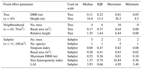
DBH denotes diameter at breast height, No. stands for “number of” and LAI is the leaf area index.

Table 2 Type, number and range of values of categorical variables used as random effects in the linear mixed effects models on the named scale.

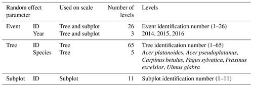
ID refers to the identification number.

We developed models at two spatial scales: (1) individual tree scale and (2) aggregated subplot scale, in both cases assessing how precipitation, tree size and neighbourhood affect stemflow. For (1) we fitted P_g, tree DBH, tree height, neighbourhood number of trees, neighbourhood basal area and neighbourhood relative height as fixed effects and precipitation event ID, event year, tree ID, tree species and subplot ID as random effects. For (2) we fitted P_g, as well as the number of trees, number of species, the Simpson diversity index, stand basal area, maximum DBH, size heterogeneity and LAI on the subplot as fixed effects and precipitation event ID, event year and subplot ID as random effects. Tables 1 and 2 summarize the fixed and random effects of both models. We grouped measured precipitation events into size classes (small: <3 mm, medium: 3–10 mm and large: >10 mm) similarly to Metzger et al. (2017). Because of the exclusion of events with a median stemflow less than 0.5 L, fewer events representative of the small and medium size class remained in our data set; therefore, we expanded the range for the small events class to 5 mm, yielding 5 small, 7 medium and 16 large events. Thus, at each scale (individual tree and subplot scales), four linear effects models were developed, three for the individual event size classes and one including all events.

2.3.3 Data selection and transformation for linear mixed effects models

All data were checked for a normal distribution and were log-transformed if necessary (stemflow volumes and tree DBH). To be able to account for zero stemflow values, one was added to the stemflow data before transformation. All data were standardized automatically using the “scale” function in R. This normalization allows for the assessment of the single effects' impacts by comparing the slopes (fixed effects) and intercepts (random effects) fitted for each factor. All tested metrics are listed in Table 1 (fixed effects) and Table 2 (random effects).

2.3.4 Model development

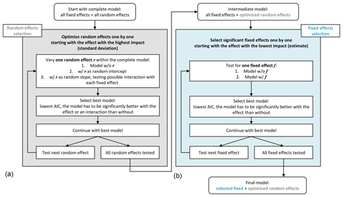
The model development involved the improvement of the mixed effects model by optimizing or excluding effects until only significant effects remained and the model had a low error. This was done successively by repeated comparison of two models which differed in one aspect only; the model that was significantly better in terms of the AIC (Akaike information criterion) was chosen. The model development was conducted here in two main steps (Fig. 2). Step (1) was the development of the random effects model: starting with a complete model including all possible fixed and random effects, the significance of random effects was tested separately for each effect. Here, selection started with the effect with the highest standard deviation, testing all possible interactions, the simple effect (no interaction) and the exclusion of the effect. Only significant random effects were retained. Step (2) was the development of the fixed effects model from the established random effects model. Here, selection started with the effect with the lowest slope estimate, testing whether the model improved significantly with inclusion of the effect. Only significant fixed effects were retained.

Figure 2 Workflow of the linear mixed effects models development steps, consisting of (a) the optimization of the random effects and (b) the selection of significant fixed effects. “w/o” refers to without and “w/” refers to with.

3 Results

3.1 Event and stemflow characteristics

We recorded 38 precipitation events with a total P_g (gross precipitation) of 626 mm (Table 3). Roughly half of the events fell into the “large” class (P_g>10 mm). Overall, only a small fraction of rainfall (1.8 %) was converted to stemflow, but the contribution changed with event size (Fig. 3). Small and medium events (50 % of the events) only contributed 4 % of total stemflow in our study area. Most of the stemflow (96 %) was derived from events classified as “large”. Moreover, 80 % of the stemflow was generated in the largest 30 % of events, and 30 % of the total measured stemflow was generated in one single large precipitation event of 65 mm (30 May 2014).

Table 3 Overview of collected stemflow precipitation events. Measured stemflow depth refers to cumulative stemflow of one event of all trees that could be evaluated. Events that were excluded from the linear mixed effects modelling are labelled and the reason for the exclusion is given (see Sect. 2 for more detail). Gap-filled stemflow is only available for events included in the modelling analysis. The overall gap rate was 6.2 %, missing a mean of 5.2 % of the calculated total stemflow. The date format is month/day/year.

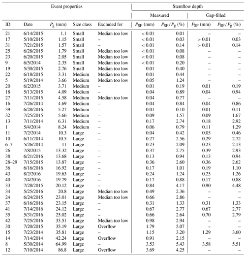
P_g refers to gross precipitation, and P_SF is stemflow net precipitation.

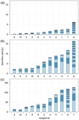
Figure 3 Ranked cumulated subplot of stemflow (bars) per event for each event size class: a small, <5 mm; b medium, 3–10 mm; and c large, >10 mm. The contributions of individual trees are also shown (alternating light and dark blue sections of each bar).

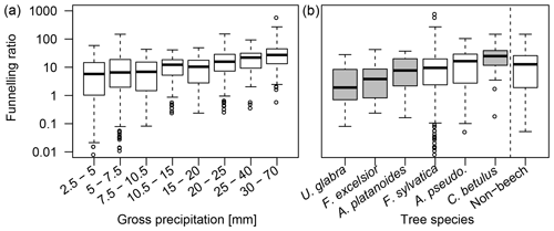
Figure 4 Event funnelling ratios of individual trees (n=65), in relation to (a) event gross precipitation and (b) tree species. Grey shaded boxplots contain the data of less than three individual trees.

Event funnelling ratios increased with event size (Fig. 4a) from a median of 1 for small events to a median of 7 for medium events and 14 for large events. Maximum values range from 60 for events with a rainfall of less than 30 mm to over 200 for the largest recorded event with a rainfall of 65 mm. As funnelling ratios increase with event rainfall, local input near stems increases relative to gross precipitation with event size. Thus, large events not only contribute most to total stemflow, but additionally enhance the funnelling effect. Non-beech trees on our plot are as productive on average as the beech trees (Fig. 4b).

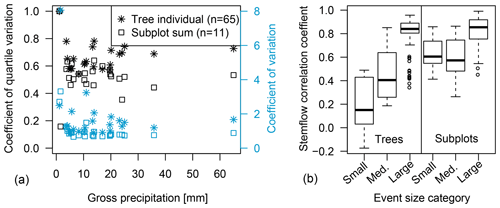
Figure 5 (a) Coefficients of quartile variation and coefficients of variation for stemflow of individual trees as well as subplots for all recorded precipitation events in relation to gross precipitation. (b) Temporal stability of stemflow on the tree scale and the subplot scale, calculated as pairwise correlation coefficients (Spearman) of tree/subplot stemflow between all of the different precipitation events of one event size class.

The coefficient of quartile variation (CQV) for all events averaged out at 0.65, for large events it increased to 0.7. Between subplots, variation for all events as well as for large events amounted to 0.55 (Fig. 5a).

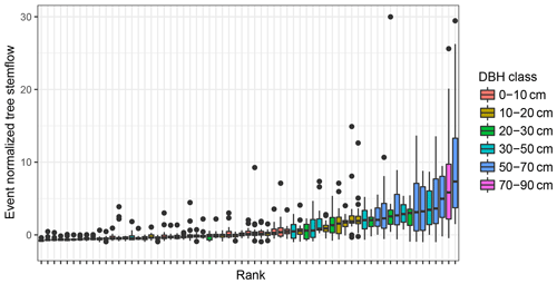
Figure 6 Temporal stability of individual tree stemflow over all sampled events. Trees are ranked according to their median event normalized stemflow and coloured according to DBH (diameter breast height).

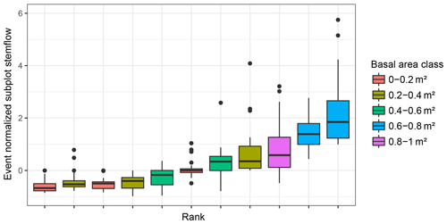
Figure 7 Temporal stability of 100 m² subplot stemflow over all sampled events. Subplots are ranked according to their median event normalized stemflow and coloured according to basal area.

Spatial patterns of stemflow were temporally stable (Figs. 5b, 6, 7). This is especially true for large rainfall events (Fig. 5b). The median correlation coefficient between stemflow in events of the large event class is 0.9 and is significantly (p≪0.001) higher than in small or medium events both on the tree and the subplot scale. This indicates that systematic drivers of stemflow are active for large events at both scales. Additionally, higher stemflow ranks did not always correspond to higher DBH ranks (Figs. 6 and 7).

3.2 Site, vegetation and neighbourhood factors affecting stemflow

3.2.1 Individual tree models

All linear mixed effects models for individual tree stemflow cover much of the variation in observed stemflow yields (R²=0.77–0.91, Table 4). However, for medium events, most of the variance is explained by the random effects, which implies that the non-measured individual and site properties had a large overall effect on stemflow, whereas included factors were not as important.

Table 4 Results of the linear mixed effects models for individual tree stemflow yield: slope estimates and significance levels of significant fixed effects, standard deviations of random effects and their interacting fixed effects (random slopes). The four models include (i) all precipitation events, (ii) small precipitations events with less than 5 mm of rainfall, (iii) medium precipitation events with between 3 and 10 mm of rainfall and (iv) large precipitation events with more than 10 mm of rainfall. Pseudo-R² values are given for each full model (fixed and random effects), for the fixed effects model separately and for the random effects model separately. Note that data were scaled before model development.

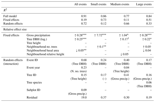
¹ Effect was not significant, but was necessary for the model's convergence. DBH represents the diameter at breast height; log. refers to log-transformed; no. refers to “the number of”; n. stands for neighbourhood; precip. is precipitation; rel. refers to relative.
The levels of significance are as follows: ${}^{\ast \ast \ast }$: p<0.001; ${}^{\ast \ast }$: p<0.01; ^∗: p<0.05; ^.: p<0.1.

Considering modelled fixed effects, as expected, event rainfall (P_g) is the most important and significant effect in all event size classes (Table 4). For small and medium events, P_g explains most (99 % and 83 % respectively) of stemflow in the fixed effects. However, for large events, P_g is less important whereas tree size (i.e. DBH) becomes more important: 48 % of stemflow is explained by P_g and 37 % is explained by DBH in the fixed effects in large events.

Neighbourhood properties (number of trees, basal area or relative height) have a significant impact on stemflow for the small events, and they are a trend in medium and large events (p=0.077 and 0.055 respectively). The neighbourhood parameters that are important vary with the event class, whereas the direction of the effects (i.e. increasing or decreasing stemflow) is consistent in all event classes. Neighbourhood effects increase with event size from small to large events, while gross precipitation concurrently decreases from small to large events. Thus, neighbourhood properties affect stemflow more strongly for large events. During large events, the number of trees in the neighbourhood increases stemflow, whereas stemflow is decreased by a larger basal area and taller trees in the neighbourhood. Overall, neighbourhood “crowding” (i.e. parameters indicating high biomass, like neighbourhood basal area) tends to decrease stemflow production per tree with one notable exception: the number of trees in a neighbourhood increases stemflow yield.

Additional neighbourhood effects may be hidden in the random effects which encompass unquantified but systematic effects of repeated measurements within a group or individual. Of those, subplot ID is almost never significant (Table 4). Instead, event ID is the strongest random effect for all models, accounting for rain event characteristics not captured by total event rainfall. The interaction with tree diameter shows that the prominent relationship between tree diameter and stemflow changes with the individual event properties. The second strongest effect is tree ID, which acts as proxy for tree parameters other than those quantified in the fixed effects, e.g. tree morphological features. Interaction of P_g with tree ID indicates that individual trees may yield more or less stemflow, depending on the event precipitation. Furthermore, tree species is only a significant random effect for large events, interacting with DBH, showing that the relation between DBH and stemflow is species-specific. Event year only appears in the model for medium sized events with a very small contribution. Overall, the random effects reflect the substantial importance of tree properties other than DBH for generating stemflow, specifically individual tree morphology and position (tree ID) and tree species.

3.2.2 Subplot-scale models

All mixed effects models for subplot stemflow explain a large proportion of variance, which are higher than for the individual tree models above (R²=0.85–0.95, Table 5). Similar to the individual tree models, in medium events, the random effects explanation more of the variance than the fixed effects.

Table 5 Results of the linear mixed effects models for subplot stemflow: slope estimates and significance levels of significant fixed effects, standard deviations of random effects and their interacting fixed effects (random slopes). The four models include (i) all precipitation events, (ii) small precipitations events with less than 5 mm of rainfall, (iii) medium precipitation events with between 3 and 10 mm of rainfall and (iv) large precipitation events with rainfall more than 10 mm of rainfall. Pseudo-R² values are given for each full model (fixed and random effects), for the fixed effects model separately and for the random effects model separately. Note that data were scaled before model development.

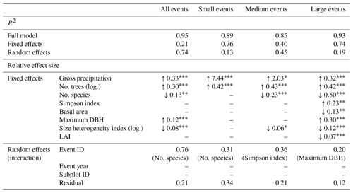
“no.” refers to “the number of”; log. refers to log-transformed; DBH is the diameter at breast height; LAI is the leaf area index; ID is the identification number.
The levels of significance are as follows: ${}^{\ast \ast \ast }$: p<0.001; ${}^{\ast \ast }$: p<0.01; ^∗: p<0.05; ^.: p<0.1.

P_g and the number of trees on the subplot are the most important fixed effects (Table 5). Their relative contribution shifts from small and medium events to large events, with P_g losing and number of trees gaining importance (ca. 95 % and 5 %, 75 % and 15 %, 15 % and 20 % for small, medium and large events respectively). For all event sizes, P_g, number of trees and maximum DBH increase stemflow, whereas subplot basal area, LAI and most of the diversity measures (both number of species and size heterogeneity index) decrease it. The exception is the Simpson species diversity index, which also increases subplot stemflow.

Only one random effect, event ID, is significant for all subplot models (Table 5). Neither event year nor subplot ID played a role in any of the models, indicating that plot properties were sufficiently captured by the fixed effects. This is further supported by the high proportion of fixed effects contributing to the explained variance, specifically in large events (R²=0.93, thereof 0.74 for the fixed effects model and 0.19 for the random effects model, Table 5).

3.2.3 Comparison of tree- and subplot-scale models

At both the individual tree and subplot scales, the model encompassing all events was dominated by the random effects, although in both small and large events most of the variance was explained by (different) fixed effects. This shows that driving factors differ between event size classes; therefore, we will focus mainly on event class models.

Generally, R² values are higher for the subplot than for the individual tree model. Thus, the subplot-scale model was better able to explain the data variation. Moreover, the R² values of the fixed effects are higher at the subplot scale, whereas the R² values of the random effects (as well as the model residual within the random effects) were higher in the individual tree model.

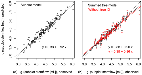
Figure 8 (a) Predicted stemflow per subplot using the subplot linear mixed effects model in relation to observed values for the large event class. (b) Stemflow sums per subplot predicted by the individual tree linear mixed effects model in relation to observed values. Panel (b) additionally shows the predicted values when excluding the tree ID random effect from the individual tree model. Dashed lines give the one-to-one line, continuous lines show the linear regressions and equations are given in the graph.

The regression slopes between predicted and observed data are slightly smaller than 1 at both scales, indicating a bias towards underestimation (see the example for large events in Fig. 8). The model bias of the subplot model (slope of 0.92) is lower than that of the individual tree model (0.87). Consequently, when calculating subplot stemflow from individual tree model predictions, the prediction bias is slightly worse (slope of 0.9) than that of the subplot level model itself (Fig. 8). The same procedure allow for the evaluation of the role of the tree ID at the subplot scale. Remember that the tree ID in the individual tree models could potentially include neighbourhood effects, specifically morphology (enhancing individual stemflow without affecting the neighbour) or shading (enhancing individual stemflow at the expense of the neighbour). For this, we calculated subplot sums of stemflow predicted by the individual tree model with and without including the tree ID random effect in the model. The regression slope for the prediction without the tree ID was only 0.86 (vs. 0.9 with the tree ID included, see Fig. 8). The difference is not significant but a trend exists, showing that tree ID contributes to increasing stemflow in one (or several) individuals on the subplot without decreasing it in others.

In general, similar patterns emerge for different event size classes at the tree scale and at the subplot scale: P_g is a strong driver for stemflow at both scales and loses influence with increasing event size, although more so at the plot scale. Instead, tree or stand characteristics affect stemflow, especially in large events. On both the individual tree and subplot scale, absolute tree size and the number of trees most strongly increase stemflow, whereas neighbourhood/subplot basal area slightly decreases stemflow. Species become relevant at both scales especially for large events. Event ID is the strongest random effect on both scales, whereas subplot ID was not significant as a random effect at either scale.

However, we also observe small differences between the individual tree- and subplot-scale model patterns: for individual tree models, apart from P_g, individual tree size is most important for large events and neighbourhood effects play a minor role. In contrast, for the subplot model, several stand structural parameters affect stemflow. Especially, the number of species and the number of trees are more important than P_g and tree size. Notably, while the size heterogeneity index significantly decreases stemflow for large events at the subplot scale, we found no effect of the equivalent measure (relative height) on the individual tree scale.

4 Discussion

Stemflow varied substantially in space both at the individual tree as well as at the subplot scale. At the same time, the greatest share of stemflow volume was created during large events, when spatial patterns of stemflow were particularly temporally stable, both at the individual tree as well as at the plot scale. This shows that in addition to throughfall, the temporal stability of which has been repeatedly reported, stemflow patterns are equally or even more stable in time (Metzger et al., 2017). Furthermore, funnelling ratios increased with increasing event size. Our findings confirm that (i) spatial patterns in stemflow are systematic and can therefore be explained by tree or stand properties, which we try to identify in this study, and (ii) large events generate the majority of total stemflow, have the highest funnelling ratios, and spatial patterns are the most pronounced and stable.

4.1 Tree size only affects stemflow during large events with fully developed flow paths

Tree metrics are the most important fixed effects for large events (but are less important for small events), which is likely related to the establishment of fully connected stemflow paths. Fully connected flow paths lead to the built-up of stable, systematic patterns of stemflow and increased funnelling ratios, relating strongly to tree properties. This agrees with previous research on stemflow generation processes: although some studies conceptualized stemflow invoking a bucket concept, where tree (André et al., 2008) or bark (Aboal et al., 1999) storage need to saturate before stemflow is initiated, a more dynamic picture is given by Herwitz (1987), Crockford et al. (1996), Levia and Frost (2003) and Levia et al. (2010) which fits well with our observation. Levia and Frost (2003) state that “stemflow generation can begin before the woody frame is completely wetted” due to preferential flow lines resulting from tree morphology or angled rain. Levia et al. (2011) and Van Stan et al. (2016) go one step further, describing the development of new flow paths with progressing rainfall duration, as additional tree surfaces are wetted. Additionally, Levia et al. (2010) observed higher delays in stemflow channelling at rainfall variation for larger trees of the same species. In either of these cases, stemflow generation depends on critical event size thresholds. This view is supported by our findings: for small events, factors shaping spatial stemflow patterns are mostly random and of low temporal stability, indicating that flow paths are not yet well established. Medium events are characterized by increased temporal stability of spatial ranks, but low explained variance in the fixed effects, indicating that flow paths are only partly developed. For large events, tree traits related to water collection or channelling capability are the most important factors explaining individual tree stemflow, which indicates that flow paths are fully established. Together, these results suggest that increasingly established flow paths with increasing event size invoke spatially stable patterns of stemflow that are more related to tree attributes and less to event properties.

4.2 Neighbourhood and stand properties affect stemflow

4.2.1 Stand structure effects largely explain subplot stemflow

For large events, all proposed stand structural parameters are significant at the subplot scale. Subplot ID has no random effect; thus, selected stand characteristics in the fixed effects capture the stemflow generation processes on the subplot scale well, also including those unexplained morphological factors which are hidden in the tree ID on the individual tree scale. Furthermore, the subplot-scale model explains more variance than the individual tree model.

For large events on the individual tree scale, neighbourhood effects only appeared as trends, which may have been related to different neighbourhood variables, such as number of trees vs. basal area, working in different directions. However, the subplot models reveal that those neighbourhood effects identified at the individual tree level act in the same way at the subplot level: the number of trees still increases the stemflow on the subplot level, whereas basal area reduces it. This shows that a tree's neighbours systematically affect its stemflow and that those patterns do not cancel each other out when considering community stemflow at the subplot scale. Moreover, this suggests that the tree morphologic properties hidden in the tree ID on the individual tree scale are actually associated with stand and neighbourhood dynamics.

It is not surprising that stand structure in a recruiting forest is organized in a patchy fashion. Due to the enormous competition for light a climax forest cannot regenerate, except in spatial and temporal niches, e.g. due to the invasion of clearings due to the death of mature trees or other environmental heterogeneities (Horn, 1971). Consequently, regeneration patterns in an undisturbed forest, like the one observed here, organize into a juxtaposition of patches with different stand ages, species compositions and structures. This structural mosaic is also obvious from the variation in our subplot-scale stand metrics and our data suggest that it propagates to ecohydrological functioning.

In conclusion, neighbourhood effects were better covered by subplot properties than by the metrics of the individual neighbourhood. Accordingly, knowledge of stand structure proves to be advantageous for stemflow assessment.

4.2.2 Tree density positively affects stemflow, while shading plays a subordinate role

Number of trees is the most prominent positive contributor to stemflow on the subplot level, confirming the intuitive rule that more trees produce more stemflow. Similarly, Reynolds and Henderson (1967) found higher interception in denser stands, which potentially becomes stemflow after a certain rainfall threshold. Accordingly, Molina and Del Campo (2012) report increased stemflow for higher stand densities. Levia and Frost (2003), Levia and Germer (2015) and Levia et al. (2015) argue that more woody surface area (hit by raindrops and providing stemflow pathways) is a main prerequisite for enhanced stemflow. This implies that – next to bigger trees or trees with more branches – a higher number of trees also potentially increases stemflow. Interestingly, the number of trees in the neighbourhood also increases individual tree stemflow, which is far less intuitive than the equivalent at the subplot scale. The number of neighbours could also enhance a tree's stemflow by promoting steeper branching angles in dense stands (Schröter et al., 2012; Juchheim et al., 2017), which are known to yield more stemflow (Návar, 1993; Levia et al., 2015, see below). Molina and del Campo (2012) similarly observed increased stemflow production in denser stands at the individual tree scale in a Mediterranean climate but attributed the effect to evaporation protection under dense canopies, as they varied density in their study by thinning and could therefore exclude canopy morphology as a reason. Alternatively, dripping on smaller trees may contribute to stemflow generation (see below).

In additional to higher tree density, reduced leaf area also increased stemflow, potentially by increasing the exposed woody surface. This agrees with former studies on the effect of tree properties on stemflow generation (Van Stan and Levia, 2010; Takahasi et al., 2011; Molina and del Campo, 2012; Levia et al., 2015); rain intercepted by leaves is rather redirected away from the stem and becomes throughfall, as leaves are not steeply inclined toward the branch, especially when they are wet.

The most frequently proposed direct neighbourhood impact in the literature is a rain shading effect, where exposed canopies collect more precipitation than less exposed ones (Takahashi et al., 2011; Terra et al., 2018). André et al. (2008) discussed the fact that small trees overtopped by larger neighbours might be deprived of a great part of rainfall. Similarly, amongst others (Crockford and Richardson, 1990; Návar, 1993; Aboal et al., 1999), Levia and Frost (2003) found higher stemflow production in the upper canopy. However, in Reynolds and Henderson (1967), medium height, co-dominant and subdominant trees were the most efficient with respect to stemflow production. Pointing in the same direction, smaller trees are often reported to have higher stemflow funnelling ratios (Murakami, 2009; Van Stan and Levia, 2010), and our data support this.

Relative height as a fixed effect was never significant in our models. In contrast, the combination of number and size (basal area) of neighbouring trees impact a single tree's stemflow. Our data also suggest that the highest or largest tree does not automatically yield the most stemflow (tree height was not retained in the tree-scale model and ranks of DBH and stemflow yield are not the same). The highest trees are the best competitors for light, which implies tree traits which are not beneficial for stemflow production: small crowns, few branches and a low DBH per height ratio (Juchheim et al., 2017). Moreover, thick leaf layers in the light canopy could divert rainfall from the tree, as a high LAI reduces stemflow production (see above).

In conclusion, stemflow is enhanced by tree density, and is limited by trade-offs between trees when basal area increases. Thus, we find the positive impact of tree density much stronger than the shading effect between trees, which, in contrast, is much weaker than expected.

4.2.3 Neighbourhood influences stemflow indirectly by shaping tree morphology

Apart from the neighbourhood effects revealed by those factors characterizing the neighbourhood (as discussed above), there is a “dark figure” of potential neighbourhood interactions hidden in the random effects at the tree scale, specifically event year, tree ID and subplot ID. The year of the measurement covers canopy dynamics as growth and canopy gaps due to windfall and broken branches, changing both the tree and its neighbourhood. The subplot ID represents the properties of the small tree community that the respective tree is situated in which are not covered by the fixed effects describing the neighbourhood. The tree ID comprises all kinds of tree traits (canopy architecture) and canopy position effects (shading or exposure) which are not covered by the fixed effects.

Of those random effects, tree ID is the most prominent significant random effect in all event classes. Interestingly, when predicting subplot-scale stemflow using the individual-scale model for large events, the subplot stemflow is underestimated, and more so than by predicting the subplot stemflow using the subplot-scale model. Therefore, the tree ID-induced variance at the tree scale does not cancel out at the subplot scale. This further supports the conclusion that interactions are not shading, but more likely stemflow-enhancing tree morphology effects.

Neighbourhood impacts stemflow indirectly, as it shapes the growth of a tree's canopy (Horn, 1971; Schröter et al., 2012; Juchheim eta l., 2017) and stands representative for small tree communities, as species and ages do not mix randomly, but appear in clusters. At the same time, the morphology of a tree substantially affects stemflow: Aboal et al. (1999) found, that bigger crown projection area, the position in the canopy and smoother bark yielded higher stemflow volumes. Návar (1993) reported higher stemflow yields for trees with many, steeply inclined branches from the top part of the crown. Iida et al. (2005) attributed branching angles to changes in precipitation partitioning and more branches and, thus, higher crown length to higher stemflow. In a study on beech saplings, Levia et al. (2015) identified, from a set of properties, besides woody surface, more and steeper branches and fewer leaves as significantly promoting stemflow.

As every tree is a dynamic imprint of its direct environment, the neighbourhood and its temporal development drive a tree's traits. Our results suggest that this reflects on stemflow yield. Additional measurements of canopy architecture would be required to confirm the potential effects of stand density on tree morphology in our plot.

4.3 Tree diversity increases stemflow, possibly due to effective canopy space occupation

Most of the parameters capturing the diversity and heterogeneity of the stand decrease stemflow, with the notable exception of the Simpson index. This may be related to the fact that our forest plot is beech dominated, and the fully grown beech trees concurrently produce a great deal of stemflow (André et al., 2008; Krämer and Hölscher, 2009; Van Stan and Levia, 2010).

Our results are in line with observations by Krämer and Hölscher (2009), who found a decrease in stemflow with species diversity (Shannon index) in a nearby forest and attributed this result to the high beech proportion at their site being a strong driver for stemflow. Schroth et al. (1999) also observed reduced stemflow in mixed stands, although they argued that this finding would strongly depend on the species involved and their traits

However, in forest stands dominated by stemflow-prolific tree species, increasing stand heterogeneity implies both a decrease in tree size and introduces less stemflow-producing species. Thus, heterogeneity measures need to be interpreted with caution, especially when measurements from representative trees are used.

The parameter “number of species” rather reflects a reciprocal of the number of large beech trees on the subplot than a measure of species richness. This is because most trees (80 %) are beech and the number of species is strongly related to the number of small trees (DBH ≤0.11 m, R²=0.88) on the subplots. Moreover, size heterogeneity reduces stemflow generation during medium and large events. Stronger size heterogeneity implies the coexistence of both very large and very small individuals, where, in terms of stemflow, the smaller individuals potentially add little to the effect of the prolific large tree(s).

Furthermore, Juchheim et al. (2017) showed a significant change in beech morphology when mixed with other species, of a kind potentially enhancing stemflow. Therefore, intermixture of other tree species in beech-dominated forests may have a positive impact on stemflow production, specifically for the beech trees, but not necessarily for the intermixed non-beech trees.

Notably, the Simpson index at the subplot scale is positively related to stemflow. The Simpson index is a relative measure of species diversity that corrects for the number of individuals considered (Buckland et al., 2005). The Simpson index illustrates not just the mere number of species, but the balanced species abundance; therefore, it is sensitive to the strong beech dominance that we find on most subplots (Magurran, 2004). The Simpson index only significantly increases stemflow for large events, where flow paths are established, and individual tree trait effects on stemflow develop their full potential. Frech et al. (2003) showed that more diverse tree communities are very efficient in using the canopy space. As different species use different strategies to compete for resources, they form variable canopy shapes which makes it easier for trees of different species to move closer together. A more efficient occupancy of canopy space increases woody surface area, the existence and exposition of which has been shown to be the core of stemflow promotion (see above, Levia and Frost, 2003; Levia and Germer, 2015; Levia et al., 2015). Additionally, beech trees growing in concert with other species are more likely to develop crown morphologies with a higher number of branches (Juchheim et al., 2017), which further promotes stemflow (Levia et al., 2015).

5 Conclusion

In this study, we investigated possible neighbourhood effects on stemflow yield on the individual tree and subplot (patch) scale. Our unmanaged and mixed-species forest produced a high spatial variance in individual tree stemflow. Spatial patterns of stemflow were temporally stable, especially for large events. The spatial variance persisted with the same order of magnitude on small forest patches of 10 m × 10 m.

Tree size was not the only relevant trait for stemflow generation. Neighbourhood and stand properties contributed importantly to stemflow distribution. On both investigated scales, stemflow increased with the number of trees in the neighbourhood. Tree density particularly increases woody surface area – a key to stemflow promotion, providing rain receiving area and flow paths. Because neighbourhood effects did not cancel out at the subplot scale, tree morphology (crown architecture) must have enhanced subplot stemflow. As canopies react plastically towards their surroundings, neighbourhood impacts tree morphological features, including those affecting stemflow. In contrast, shading within the canopy was much less important: relative height did not affect stemflow, only neighbourhood and stand basal area, representing larger trees, slightly reduced stemflow which suggests a weak shading effect. Furthermore, barely decreased stemflow variance at the subplot scale indicates that shading effects are probably minor.

All impacts are most obvious for large precipitation events. Tree, stand and neighbourhood effects are more important as event size increases. We conclude that the full development and connection of drainage flow paths through the canopy taps the full potential of systematic factors in forest structure impacting stemflow yield. Because of positive effects on forest density, unmanaged and mixed-species forest could be more stemflow-productive than managed ones. This is supported by the positive effect of the Simpson diversity index on small stand stemflow. More research is required to understand systematic effects of forest management on stemflow.

Appendix A

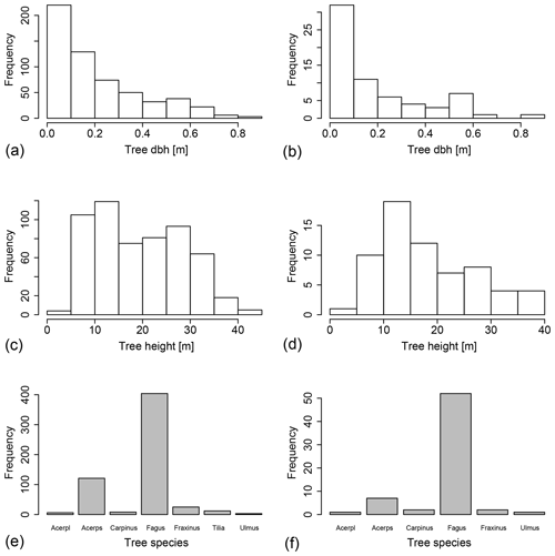
Figure A1 (a, c, e) Histograms of stand properties on the whole 1 ha plot (n=581) and (b, d, f) the 11 100 m² subplots on which stemflow was measured (n=65). “Acerpl” refers to Acer platanoides, and “Acerps” refers to Acer pseudoplatanus. Please see Table 2 for a list of the other occurring species.

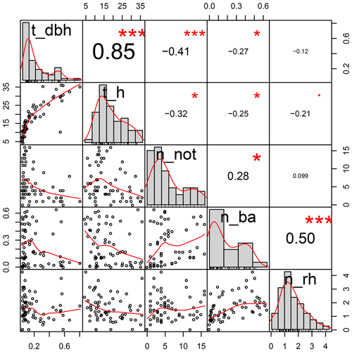
Figure A2 Distributions and correlations of variables included as fixed effects in the linear mixed effect models of individual tree stemflow. “t_dbh” refers to the tree DBH; “t_h” is the tree height; “n_not” is the number of trees in the neighbourhood; “n_ba” is the neighbourhood basal area; “n_rh” is the neighbourhood relative height; DBH is the diameter at breast height.

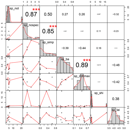
Figure A3 Distributions and correlations of variables included as fixed effects in the linear mixed effect models of subplot stemflow. “sp_not” is the number of trees in the subplot; “sp_nospec” is the number of species in the subplot; “sp_simp” is the Simpson diversity index of the subplot; “sp_ba” is the basal area of the subplot; “sp_dbhmax” is the DBH of the biggest tree on the subplot; “sp_shi” is the size heterogeneity index of the subplot; “sp_lai” is the subplot LAI; DBH is the diameter at breast height; LAI is the leaf area index.